Anti-freezing time prediction of fire pipe covered with insulation material in low temperature environment

Abstract

The reliable operation of fire pipes in cryogenic environments is essential to ensure safety in residential and industrial environments. This study introduced a systematic approach that combined experimental data, computational fluid dynamics (CFD) simulations and machine learning techniques to investigate the thermal performance of insulated fire pipes. A key contribution of this study is the derivation of a calibrated analytical expression for the heat transfer coefficient in natural convection that accounts for the dynamic effects of insulation thickness and ambient temperature. The validated CFD model was used to simulate the freezing process, while the random forest (RF) algorithm was used to predict the optimal insulation thickness to achieve a specific antifreeze time. The results showed that the type, thickness and ambient temperature of the insulation material had considerably affect the antifreeze performance, with rubber sponges outperforming aluminium silicate shells in cryogenic environments. The optimized RF model exhibited high accuracy and robustness, providing a practical tool for insulation design. This study provides valuable insights and technical guidance for improving the reliability of fire pipes under extreme conditions.

Keywords

Fire pipe insulation material anti-freezing time convective heat transfer coefficient random forest prediction

Introduction

The reliable operation of fire-fighting systems under extreme environmental conditions is critical for ensuring safety in residential and industrial settings.^1,2 Amongst these, maintaining the functionality of fire pipes during low-temperature scenarios presents a major engineering challenge.³ Fire pipes, which often remain static for prolonged periods, are particularly susceptible to freezing and subsequent damage during cold weather periods.⁴ To mitigate this risk, insulation materials are commonly employed.^5–7 However, the thermal performance of these materials and their ability to prevent freezing under diverse environmental conditions remain insufficiently understood. Therefore, it is imperative to develop an in-depth understanding of the thermal behaviour of insulated fire pipes to optimize their design and ensure their reliability in low-temperature environments.

Previous studies^8,9 focused on the economic thickness analysis of insulation materials by balancing material cost and heat loss to determine the optimal thickness of the insulation layer.¹⁰ However, this method usually ignores the dynamic changes in heat transfer characteristics of insulation materials in practical applications. For example, the heat transfer coefficient depends not only on the physical parameters of the material and on other factors, such as the thickness of the insulation layer and the ambient temperature. This coupling relationship has an important role in the anti-freezing performance of pipelines and the selection of insulation materials but it has not been systematically studied in the existing literature.^11,12

To overcome the limitations of traditional methods in complex heat transfer analysis, this study explored in depth the dynamic characteristics of the heat transfer coefficient as a function of the thickness of the insulation layer and the ambient temperature change, and derived an analytical expression for the heat transfer coefficient. The expression used the characteristic parameters of the insulation material (e.g., thickness, ambient temperature) as variables and theoretically evaluated the heat transfer mechanism of the system more precisely.

Computational fluid dynamics (CFD) modelling has proven to be a powerful tool for analyzing heat transfer processes, particularly in scenarios involving complex geometries and varying boundary conditions.^13,14 Shammazov et al.¹⁴ used the Fluent software program to simulate numerically the flow of liquefied natural gas in a pipe section with an outer diameter of 108 mm and a length of 10 m with three types of insulation coatings (polyurethane foam, aerogel and vacuum insulation pipe). Avikal et al.¹⁵ used the finite element analysis software program ANSYS to analyze the thermal insulation performance of six different materials and proposed a suitable pipeline insulation material. By incorporating the physical and thermal properties of the insulation materials, as well as environmental parameters such as ambient temperature, wind speed and humidity, the CFD model would provide a comprehensive representation of the thermal behaviour of the system. To ensure its accuracy and reliability, the CFD model was rigorously validated in this study against the collected experimental data. This validation process involved refining key parameters, including the thermal conductivity of the insulation, convective heat transfer coefficients and boundary conditions, to achieve a high degree of correlation between the simulated and observed results. Building upon the validated CFD model, parametric studies were conducted to explore the effects of varying insulation thickness and ambient temperature on the thermal performance of the fire pipes.

Recognizing the limitations of traditional modelling approaches in addressing highly nonlinear and complex relationships, this study also employed machine learning (ML) techniques to enhance predictive capacity.^16–18 Specifically, a random forest (RF) algorithm was developed to predict the required insulation thickness for achieving a specified anti-freezing time under given environmental conditions.¹⁹ RF was chosen for its robustness, interpretability and strong performance in handling nonlinear interactions amongst input variables.²⁰ Ambient temperature, properties of insulation materials and insulation thickness were used as input features for the ML model, while anti-freezing time was designated as the output. The RF model was optimized based on hyperparametric tuning to improve prediction accuracy and computational efficiency, ensuring its practical applicability in real-world scenarios.²¹

The integration of ML with traditional modelling techniques provides a powerful predictive framework that facilitates the optimal design of insulation systems for fire-fighting pipelines. By leveraging the RF model, engineers can rapidly determine the required insulation thickness to ensure the anti-freezing performance of fire pipes under specific environmental conditions. To validate the predictions, the results of the ML model were compared against additional numerical simulations and experimental data, ensuring the reliability and generalizability of the proposed approach.

Methods

Proposed method

The technical framework of this study is depicted in Figure 1, illustrating the systematic methodology employed to evaluate the thermal performance of insulated fire pipes under low-temperature conditions. The research began with the collection of experimental data on the temperature fall behaviour of insulated fire pipes. This was drawn from historical records and previous experimental studies, providing a robust basis for model development and validation. Subsequently, a CFD numerical model was established to simulate the thermal response of the system, incorporating the physical and thermal properties of the insulation materials as well as the relevant environmental conditions. To ensure the model's reliability and predictive accuracy, the simulation results were validated against the collected experimental data, enabling refinement of key parameters and boundary conditions.

Figure 1.

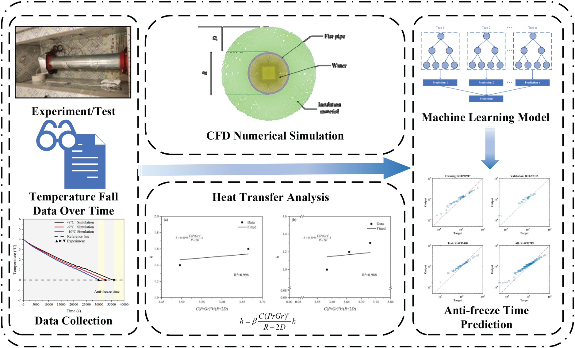
Technical route of anti-freezing time prediction.

Given the intricate nature of heat transfer during the temperature fall process, it is essential to derive an analytical expression for the convective heat transfer coefficient. This coefficient was formulated as a function of the characteristic parameters of the insulation material, enabling a more precise representation of the heat exchange mechanisms at play. The model was then utilized to conduct parametric studies by varying the insulation thickness and ambient temperature. The resulting anti-freezing time of the fire pipe under different conditions was recorded as the primary output.

To enhance further predictive capability, an ML model was developed, with ambient temperature, insulation material type and thickness serving as input features, while the anti-freezing time was designated as the output. Amongst the various ML approaches, the RF algorithm was selected owing to its robustness, interpretability and strong performance in handling nonlinear relationships. The RF model was then optimized to improve prediction accuracy and computational efficiency.

The optimized ML model was employed to predict the required insulation thickness needed to achieve a specified anti-freezing time under given environmental conditions. This predictive framework can provide a practical tool for determining the optimal design of insulation systems for fire pipes, thereby supporting decision-making in engineering applications. The accuracy of the predictions was subsequently verified through comparison with additional numerical or experimental data, ensuring the validity of the proposed approach.

Numerical simulation setup

The CFD model was developed using Fluent 2023, incorporating several key physical submodels to accurately simulate the freezing behaviour within the fire pipe,²² as depicted in Figure 2. Specifically, the Solidification/Melting model was activated to account for the phase change between water and ice. This model utilized the enthalpy-porosity formulation, where the liquid fraction was computed based on the local temperature relative to the material's melting point, dynamically capturing the solid-liquid phase transition. The Energy equation was solved to simulate the heat transfer within the pipe wall, insulation layers and the fluid domain. To clarify the computational domain, the simulation was simplified by assuming uniform properties along the longitudinal axis of the pipe, with the CFD domain restricted to the cross-section of the pipe. Given the absence of significant fluid motion, a laminar flow assumption was adopted, and natural convection effects within the pipe were neglected to simplify computation without compromising the accuracy of the freezing front prediction.

Figure 2.

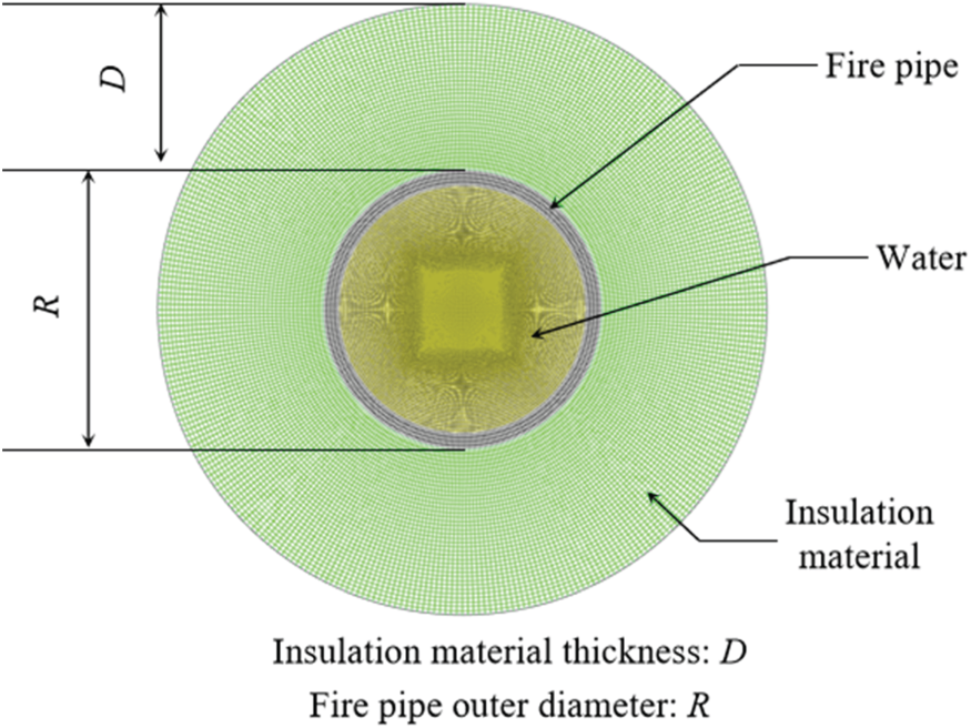
Modelling schematic of the parts and dimensions for CFD analysis.

In the present CFD model, the volume expansion associated with the phase change from liquid water to solid ice was not explicitly modelled. Specifically, the simulation assumed that the phase change process occurred under a constant volume condition, without considering the mechanical stresses or structural deformation of the pipe induced by the lower density of ice compared to water. This assumption is acceptable for the current study, as the primary objective was to investigate the thermal behaviour and freezing progression within the pipe, rather than the mechanical integrity or rupture risk of the pipe structure.

The simulation environment was set with an initial ambient temperature of 5°C. The analyzed pipe had inner and outer diameters of 150 and 159 mm, respectively. To monitor temperature changes and phase transitions during the simulation, a thermocouple and a liquid fraction sensor were strategically positioned on the inner surface of the pipe wall, enabling precise temperature measurements at key locations.

The meshing process utilized quadrilateral elements to ensure accurate geometry representation and computational efficiency. A uniform mesh size of 1 × 1 mm was adopted to achieve a fine resolution capable of capturing critical thermal gradients within the pipe. This high-resolution mesh was essential for accurately simulating the phase-change process as water within the pipe transitioned to ice under subfreezing conditions.²³

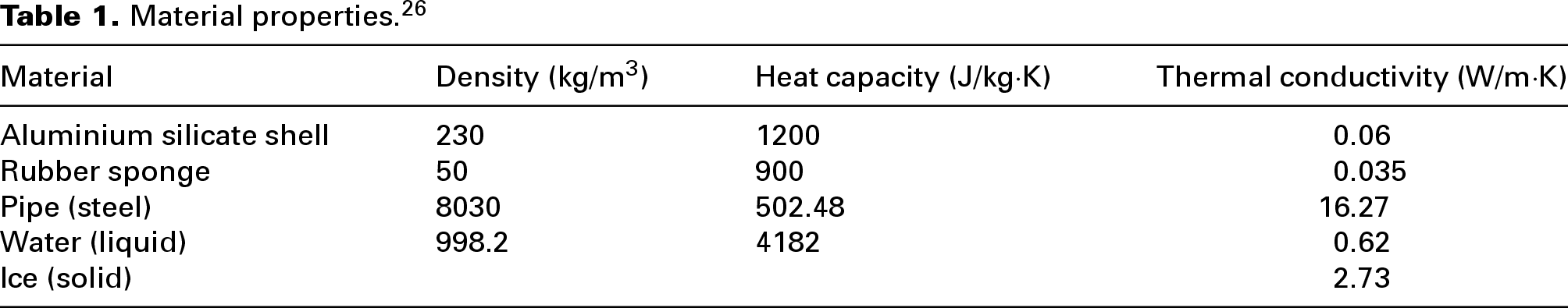
According to the experimental settings and data presented by Luo et al.²⁴ and Hao et al.,²⁵ the low-temperature experimental system used in their studies consisted of refrigeration equipment, an insulated chamber, fire pipes, a ventilation system and a temperature measurement system. This study selected two types of insulation materials, namely the aluminium silicate shell and rubber sponge. Due to the outdoor temperature fluctuated throughout the day, the experimental data used for model validation were collected under controlled conditions in the refrigeration system, which maintained a constant temperature. Table 1 provides a comprehensive summary of the material properties incorporated into the simulation. Particular emphasis was placed on the thermal conductivity of water and ice, as this parameter could influence considerably the heat transfer process. In contrast, variations in density and specific heat capacity were considered negligible and were thus not included in the analysis. This assumption was made to simplify the computational model while maintaining a high degree of accuracy in simulating the freezing process within the pipe. By focusing on the thermal conductivity differences between water and ice, the model effectively captured the dynamic thermal behaviour of the system.

Table 1.

Material properties.²⁶

Material	Density (kg/m³)	Heat capacity (J/kg·K)	Thermal conductivity (W/m·K)
Aluminium silicate shell	230	1200	0.06
Rubber sponge	50	900	0.035
Pipe (steel)	8030	502.48	16.27
Water (liquid)	998.2	4182	0.62
Ice (solid)	998.2	4182	2.73

Random forest

The RF algorithm, a prominent ensemble learning method, has achieved widespread recognition in the fields of data science and ML owing to its strong predictive capabilities and robustness.¹⁹ By constructing an ensemble of decision trees, RF can leverage the collective wisdom of multiple models to deliver more accurate and stable predictions. Each tree in the forest was trained based on a random subset of the training data, and its prediction would contribute to the final output through a majority vote for classification or an average for regression tasks. This approach would mitigate the risk of overfitting often associated with single decision trees, thereby enhancing the model's generalization ability.

Figure 3 illustrates the architecture of the RF model, highlighting how the predictions of multiple decision trees are aggregated to form a unified output. The diagram emphasizes the cooperative nature of the trees, where their combined efforts would yield a comprehensive and more reliable prediction. This structure exemplifies the power of ensemble learning, as it capitalizes on the diversity amongst individual trees to offset the weaknesses of any single model.

Figure 3.

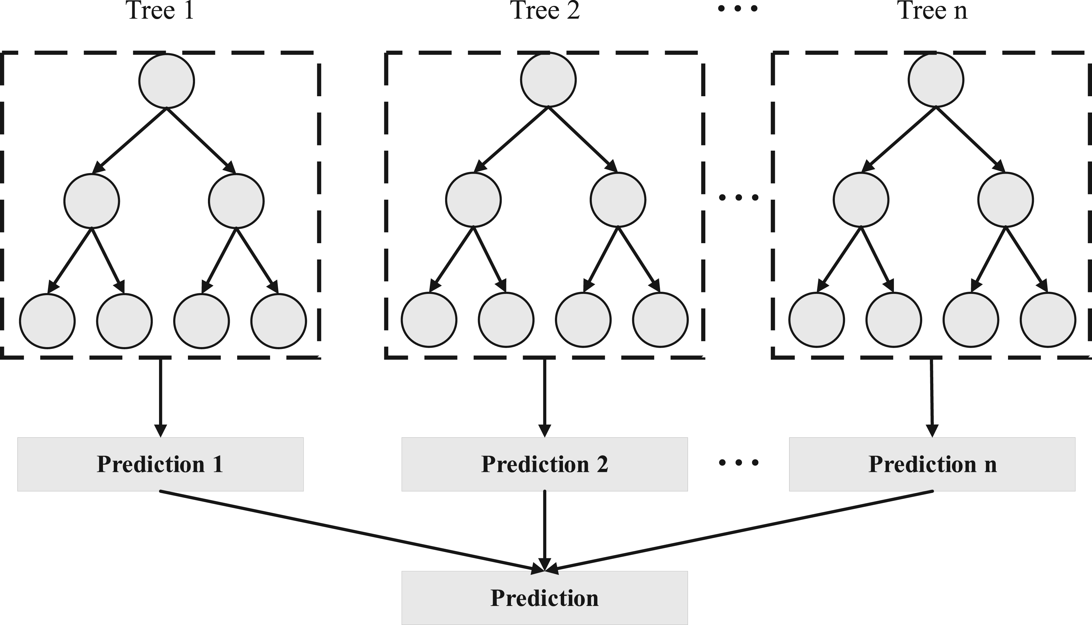
The schematic topological architecture of random forest.

Effective implementation of the RF algorithm requires careful selection of key hyperparameters.²⁷ The depth of the decision trees and the total number of trees in the forest are particularly crucial, as they directly impact the model's predictive performance, computational efficiency and capacity to generalize new data. Optimal tuning of these parameters ensures a balance between bias and variance, enabling the RF model to achieve high accuracy while maintaining robustness across diverse datasets.

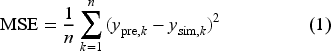
The mean square error (MSE) of the output data, calculated using Equation (1), which was utilized to evaluate the RF predictions:

\begin{aligned} MSE = \frac{1}{n} \sum_{k = 1}^{n} {(y_{pre, k} - y_{sim, k})}^{2} \end{aligned}

(1)

where y_pre and y_sim are the predicted and simulated data, respectively, and n is the number of simulated data points. The RF model, constructed using MATLAB (MathWorks, Natick, MA, USA),²⁸ was trained three times to determine the optimal parameters for each operational scenario and to compare their numerical performance.

Results and discussion

Convective heat transfer coefficient

Theoretical derivation

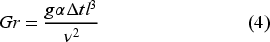
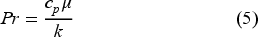
The main modes of heat transfer are heat conduction, heat convection and heat radiation.²⁹ Assuming that the fire pipe located outdoors is in a natural convection environment, the heat transfer between the numerical model and the outside world is mainly convection, and the radiation coefficient is assumed to be equal to 0.8. The natural convection heat transfer caused by the heating or cooling of the fluid by the wall is related to the buoyancy formed by the temperature difference near the wall. The uneven temperature field would cause an uneven density field and the resulting buoyancy would become the driving force of movement. The air on the hot wall is heated and floats up, while the unheated colder air sinks owing to its higher density. Therefore, during heat transfer in natural convection conditions, the fluid near the wall does not flow in the same direction as that during the heat transfer in forced convection conditions. In general, the uneven temperature field only occurs in a thin layer close to the heat exchange wall. At the wall, the fluid temperature is equal to the wall surface temperature and gradually decline to the ambient temperature in the direction away from the wall. In principle, the standard equations for natural convection heat transfer are expressed as equations (2)–(5)³⁰:

\begin{aligned} N u & = f (G r, P r) = C (G r P r)^{n} \end{aligned}

(2)

\begin{aligned} N u & = \frac{h L}{k} \end{aligned}

(3)

\begin{aligned} G r & = \frac{g α Δ t l^{3}}{ν^{2}} \end{aligned}

(4)

\begin{aligned} P r & = \frac{c_{p} μ}{k} \end{aligned}

(5)

while Nu, Gr, and Pr are dimensionless numbers, and C and n are constant terms. The variable h is the convective heat transfer coefficient, L is the characteristic length, k is the thermal conductivity of the fluid, g is the gravitational acceleration, a is the volume change coefficient, which is equal to the reciprocal of the absolute temperature for an ideal gas. Δt is the temperature difference, v is the kinematic viscosity, μ is the dynamic viscosity coefficient and c_p is the specific heat at constant pressure. Based on the expressions of Equations (2)–(5), the theoretical convection heat transfer coefficient is derived as Equation (6):

\begin{aligned} h = β \frac{C {(P r G r)}^{n}}{R + 2 D} k \end{aligned}

(6)

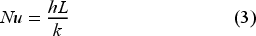
For a horizontal fire pipe, the outer surface is in an infinite space air laminar flow, where C was set to 0.48, n was set to 0.25 and the characteristic length L was set to equal to the sum of the pipe diameter (R) and two times the thickness of the insulation material (D). To calibrate the deviation between the theoretical value and the actual value, this study introduced β as the correction coefficient, which was evaluated and determined in the Section under Model verification.

Although the theoretical derivation considers the convective heat transfer coefficient as a function of temperature difference (Δt) through the inclusion of the Grashof number (Gr), which accounts for the impact of temperature on the convective heat transfer coefficient, the model in this study simplifies the process by adopting a constant convective heat transfer coefficient. This constant value was calibrated based on experimental data for specific temperature conditions.

Model verification

The test system developed by Luo et al.²⁴ included refrigeration equipment, incubators, fire ducts, ventilation systems and temperature monitoring systems. The diameter of the DN150 fire pipe was wrapped with an aluminium silicate shell insulation layer (thickness = 0.05 m), and the two sides were connected with flanges. During the test, the temperature measuring points were set at 1/3 and 2/3 of the outer wall length of the fire pipe, respectively. When the ambient air temperature was −10°C, it took approximately 15.9 h for the water temperature to cool from 5°C to 0°C. When the ambient air temperature was −12.8°C, it took approximately 12.7 h to cool down from 5°C to 0°C.

A numerical model consistent with the test device was established in the CFD software program. The boundary conditions of the model (convective heat transfer coefficient between the insulation layer and the external environment) were adjusted, and the simulation results were compared with the experimental data using a trial-and-error method. In this process, the trial-and-error approach was implemented systematically within a constrained parameter range, guided by engineering principles and thermal behaviour expectations. Rather than random attempts, each adjustment was made based on theoretical predictions and empirical observations to ensure convergence toward physically realistic values.

The results are shown in Figure 4(a) and (b) respectively. It has been verified that for aluminium silicate shell materials, the convective heat transfer coefficients at −10°C and −12.8°C are 1.4 W/(m2·K) and 1.6 W/(m²·K), respectively. The insulation material tested by Hao et al.²⁵ was a 40 mm rubber sponge, and the anti-freezing time of the DN100 fire pipe was obtained by testing at −8°C, −9°C and −10°C. Accordingly, the geometric parameters of the numerical simulation model were modified, and the same systematic trial-and-error method was applied to verify the convective heat transfer coefficients at different ambient temperatures. The results are shown in Figure 4 (c). The convective heat transfer coefficients of the rubber sponge at −8°C, −9°C and −10°C are 1 W/(m²·K), 1.2 W/(m²·K) and 1.3 W/(m²·K), respectively.

Figure 4.

Comparison of numerical simulation and experimental data: aluminium silicate shell of −10°C (a), −12.8°C (b) and rubber sponge (c).

After obtaining the convective heat transfer coefficients of the two insulation materials at different ambient temperatures, Equation (6) (derived in Section Theoretical derivation) was applied to obtain the calibration results of the convective heat transfer coeffìcients of the two materials using linear fitting, as shown in Figure 5. The correction factors (β) of the aluminium silicate shell and rubber sponge were 0.4193 and 0.3195, respectively. Although the number of data points is limited, the fitted results were based on theoretically derived models and validated simulations, ensuring the scientific validity of the fitting.

Figure 5.

Convective heat transfer coefficient calibration formula: (a) aluminium silicate shell and (b) rubber sponge.

Numerical simulation results of insulation materials

In Section ‘Theoretical Derivation’, the corrected convective heat transfer coefficients for aluminium silicate shell and rubber sponge insulation materials were obtained through theoretical analysis, simulations and experimental data. Based on these parameters, numerical simulations were performed to study the temperature fall and freezing behaviour of fire pipes under different working conditions by varying the ambient temperature, insulation material type and insulation thickness.

Type of insulation material

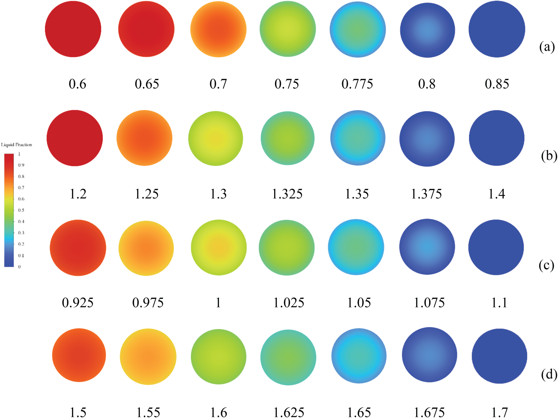
Figure 6 illustrates the temporal evolution of liquid freezing inside fire pipes insulated with two different materials – aluminium silicate shell and rubber sponge, under a low-temperature environment of −10°C. The freezing behaviour was analyzed for insulation layer thicknesses of 0.05 and 0.30 m over time, with the horizontal axis scaled by a factor of ×10⁵ s. Using the aluminium silicate shell (Figure 6(a) and (c)), the freezing process occurred more rapidly. With a thinner insulation layer (0.05 m, Figure 6(a)), freezing began at approximately t = 0.6 × 10⁵ s and was almost completed by t = 0.9 × 10⁵ s. With the thicker insulation layer (0.30 m, Figure 6(c)), freezing started slightly later but progressed quickly, achieving full freezing at approximately t = 2.7 × 10⁵ s. This indicated the high thermal conductivity of aluminium silicate, which facilitated heat transfer and accelerated freezing. The use of rubber sponge (Figuer 6(b) and (d)) exhibited considerable thermal insulation effects, delaying the freezing process. With the thinner layer (0.05 m, Figure 6(b)), freezing began later, at t = 1.0 × 10⁵ s, and was almost completed at approximately t = 1.3 × 10⁵ s. With the thicker layer (0.30 m, Figure 6(d)), freezing was delayed further, with ice formation started at t = 3.0 × 10⁵ s and was almost completed at t = 3.49 × 10⁵ s.

Figure 6.

Freeze thickness of 0.05 m (a) and 0.30 (c) aluminium silicate shell and 0.05 m (b) and 0.30 (d) rubber sponge at −10°C at different times (×10⁵ s).

Correspondingly, Figure 7 compares the anti-freezing times for both insulation materials against uninsulated conditions. Both materials significantly prolonged anti-freezing time relative to bare pipes, demonstrating effective thermal protection. Rubber sponge consistently outperformed aluminium silicate shell, especially at ambient temperatures between −10°C and −20°C. However, when the ambient temperature declined further, the difference in anti-freezing performance between the two materials was diminished, indicating that insulation effectiveness was relatively more critical in moderate low-temperature environments.

Figure 7.

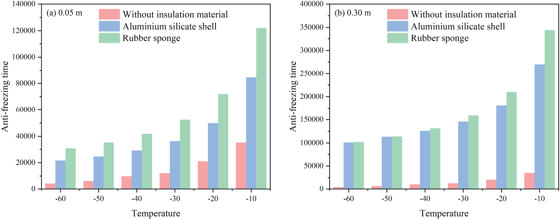
Anti-freezing time of different insulation materials with (a) 0.05 m and (b) 0.30 m.

The differences between the two insulation materials primarily due to their thermal conductivity and convective heat transfer properties. As shown in Table 1, the rubber sponge has a lower thermal conductivity, and a smaller convective heat transfer correction coefficient (β) compared to the aluminium silicate shell. This resulted in superior insulation performance and longer anti-freezing times for rubber sponge.

In summary, rubber sponge can provide a better frost protection than aluminium silicate shell under equivalent thickness and environmental conditions, mainly due to its lower thermal conductivity and reduced heat transfer rate.

Thickness of insulation material

Figure 8 illustrates the freezing evolution of liquids inside steel pipes insulated with aluminium silicate shells and rubber sponges with two different thicknesses (0.10 and 0.20 m) under a low-temperature environment of −20°C. The results show that insulation thickness could significantly affect antifreeze performance: thinner layers could promote faster freezing due to increased thermal conduction, while thicker layers could effectively delay the freezing process. The freezing dynamics over time are depicted for aluminium silicate shells (Figure 8(a) and (b)) and rubber sponges (Figure 8(c) and (d)), with the horizontal axis scaled in seconds from freezing initiation to completion.

Figure 8.

Freeze thickness of 0.10 m (a) and 0.20 m (b) aluminium silicate shell and 0.10 m (b) and 0.20 (c) rubber sponge rubber sponge at −20°C at different times (×10⁵ s).

For the aluminium silicate shell, thinner insulation (0.10 m, Figure 8(a)) would lead to faster freezing onset at approximately t = 0.6 × 10⁵ s, with complete freezing observed at approximately t = 0.85 × 10⁵ s. In contrast, thicker insulations (0.20 m, Figure 8(b)) would slightly delay the freezing process, with ice formation beginning at t = 1.2 × 10⁵ s and full freezing occurring near t = 1.4 × 10⁵ s. This indicates the role of insulation thickness in modulating the thermal transfer rate, even for a highly conductive material like aluminium silicate. For the rubber sponge, thinner insulation (0.10 m, Figure 8(c)) would delay the freezing onset to t = 0.925 × 10⁵ s, with freezing completed at t = 1.1 × 10⁵ s. The thicker layer (0.20 m, Figure 8(d)) exhibited a more pronounced delay, with initial freezing occurring at t = 1.5 × 10⁵ s and full freezing occurring at t = 1.7 × 10⁵ s. This highlighted the superior thermal insulation responses of rubber sponges, where increased thickness had reduced considerably the heat transfer and slowed the freezing process.

Figure 9 further quantifies the relationship between insulation thickness and anti-freezing time. For both materials, anti-freezing time was increased significantly with thickness, especially at higher ambient temperatures (>−30°C). At −10°C, the rubber sponge with 0.30 m thickness achieved an anti-freezing time exceeding 350,000 s, approximately 30% longer than that of the aluminium silicate shell at the same thickness.

Figure 9.

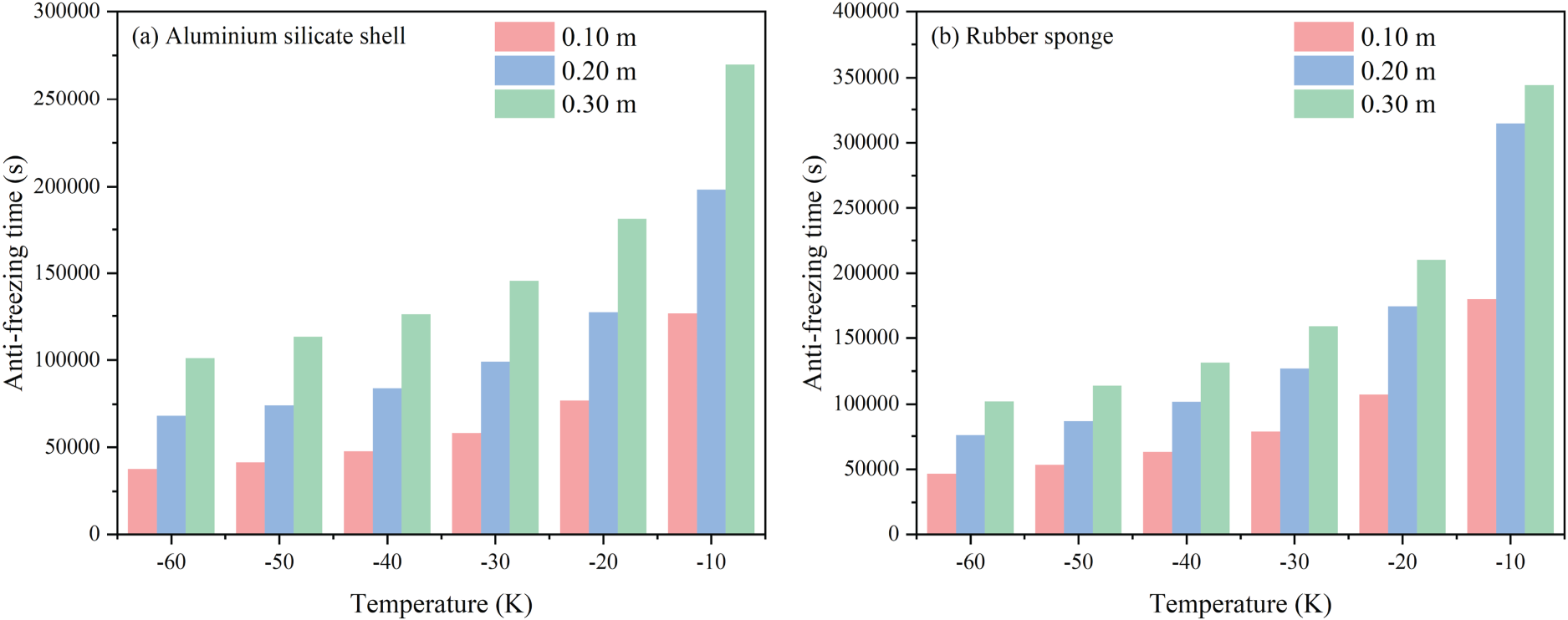
Anti-freezing time of (a) aluminium silicate shell and (b) rubber sponge with different thicknesses.

Ambient temperature

The ambient temperature has a critical role in determining the freezing dynamics of the insulated fire pipes. Figure 10 illustrates the freezing evolution for pipes insulated with 0.15 m thick aluminium silicate shell and rubber sponge at ambient temperatures of −10 and −30°C.

Figure 10.

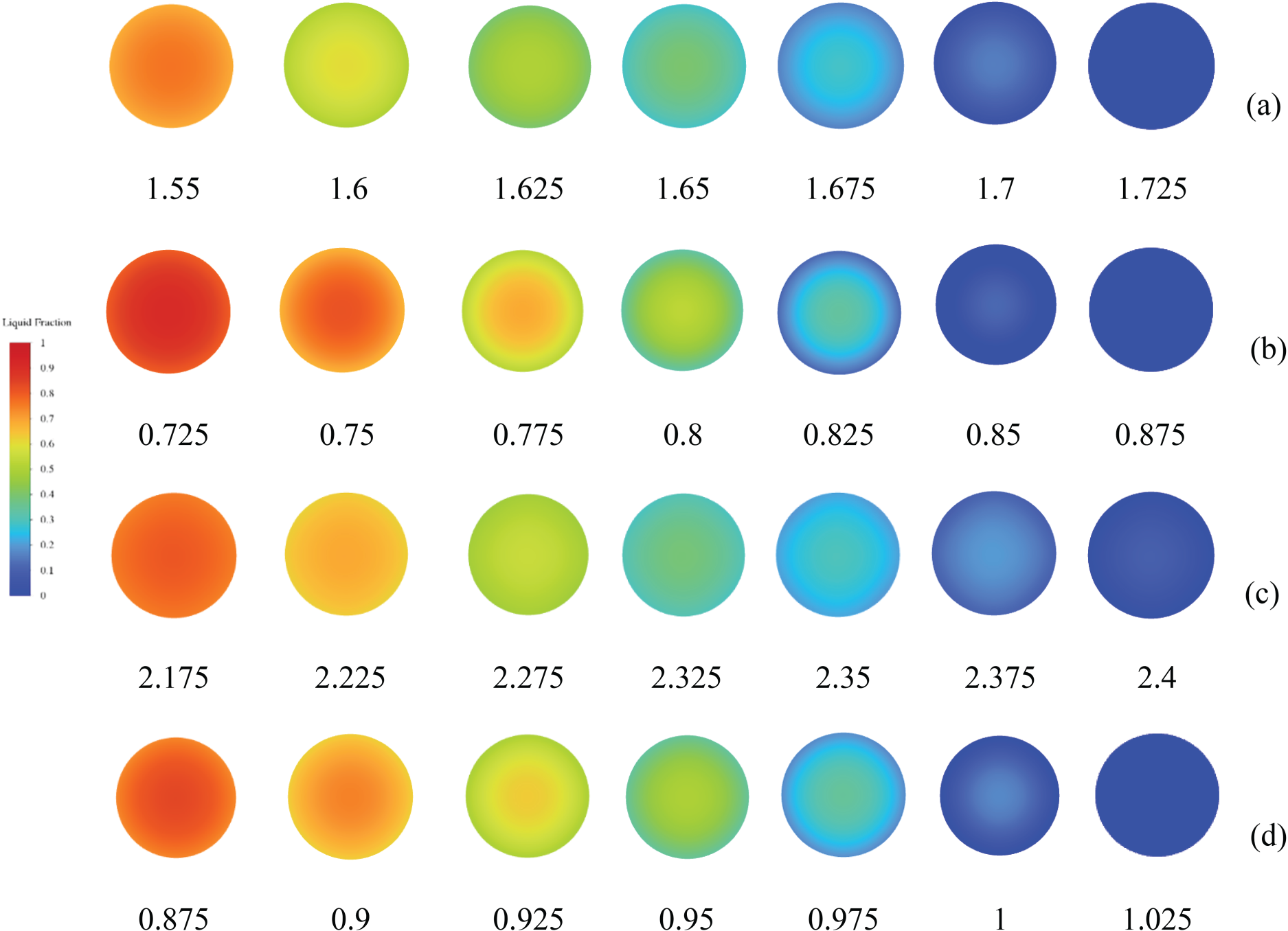
Freeze thickness of 0.15 m aluminium silicate shell at −10°C (a) and −30°C (b) and 0.15 m rubber sponge −10°C (c) and −30°C (d) at different times (×10⁵ s).

At −10°C, freezing started at approximately t = 1.55 × 10⁵ s and was completely frozen at approximately t = 1.725 × 10⁵ s using the aluminium silicate shell for insulation (Figure 10(a)). Similarly, with the use of rubber sponge for insulation (Figure 10(c)), the freezing onset was delayed considerably, starting at approximately t = 2.175 × 10⁵ s and completing at approximately t = 2.4 × 10⁵ s. This suggested that at higher ambient temperatures, lower thermal gradients would slow down the freezing process, especially for low-thermal conductivity materials, such as rubber sponges.

At −30°C, the freezing process was accelerated owing to the increased thermal gradient. When using the aluminosilicate shell for insulation (Figure 10(b)), freezing started earlier at t = 0.725 × 10⁵ s and completely frozen at t = 0.875 × 10⁵ s. For the rubber sponge (Figure 10(d)), freezing started at t = 0.875 × 10⁵ s and completely frozen at t = 1.025 × 10⁵ s. The larger temperature difference at −30°C shortened considerably the freezing times with the use of either material, although the rubber sponge could still yield a considerable delay compared with the aluminosilicate shell.

Figure 11 shows the variation of the unfrozen times with different thicknesses (0.05–0.30 m) of aluminosilicate shell (Figure 11(a)) and rubber sponge for insulation (Figure 11(b)) and ambient temperatures (−60°C to −10°C). At lower temperatures (−60°C to −40°C), the increase in anti-freezing time with thickness was relatively modest and linear. However, at higher ambient temperatures (>–40°C), the antifreeze time was increased sharply with thickness, emphasizing the more significant role of insulation in moderately cold environments. Comparative analysis shows that aluminium silicate shell could offer a slightly better unfreezing resistance than rubber sponge at extremely low temperatures (<–30°C), but rubber sponge was the superior choice for applications providing extended frost protection under typical low-temperature conditions.

Figure 11.

Anti-freezing time of (a) aluminium silicate shell and (b) rubber sponge at different temperatures.

Establishment and optimization of RF

The model used ambient temperature, insulation material correction coefficient and insulation thickness as input features and anti-freezing time as the output target. These features were selected because they are the primary environmental and structural parameters that govern the freezing process in insulated pipes under low-temperature conditions. The dataset was randomly divided into training, validation and test and was set with a ratio of 6:2:2. The training set was used to fit the model, the validation set was used for hyperparameter tuning, and the test set was used to evaluate the final model performance. Hyperparameter optimization was performed using the grid-search method. The number of leaves was set within the range of 50–200, and the maximum depth of the trees within the range of 5–20. The optimal model parameters were determined to be 150 trees and a maximum depth of 15.

Figure 12 presents the fitting results of the anti-freezing time prediction based on the Random Forest (RF) model, including scatter plots for the training set, validation set, test set and overall dataset. In each plot, the horizontal axis represents the target value (Target), and the vertical axis represents the model prediction value (Output).

Figure 12.

Performance of optimized RF model.

The model performance was characterized by the regression coefficient R, with R-values of 0.96917, 0.95315, 0.97400 and 0.96719 for the training, validation, test and overall datasets, respectively. These values were all close to 1.0, demonstrating high fitting accuracy across all data subsets. To further verify the reliability and generalization ability of the model, the predictive performance on the training and test sets was compared. The R-value on the test set (0.97400) was very close to that of the training set (0.96917), and the mean squared error (MSE) on the test set was as low as 0.017. This strong consistency between training and testing performance indicated that the model effectively avoided overfitting and maintained high accuracy on unseen data.

Additionally, the scatter points were closely distributed along the diagonal line in all subsets, suggesting a high degree of agreement between predicted and actual values and minimal prediction error. The slightly higher R-value on the training set was consistent with the typical behaviour of RF models, where the model fitted the training data slightly better than unseen data without causing significant overfitting. Moreover, the overall dataset R-value (.96719) further confirmed the model's strong robustness and its reliable predictive capability across diverse operating conditions. These results collectively had validated the effectiveness and generalization strength of the RF-based anti-freezing time prediction model.

Prediction of anti-freezing time with RF

Figure 13 shows the results of the optimized RF model for predicting the frost protection times using aluminium silicate shell and rubber sponge for insulation with different thicknesses (0.05–0.30 m) and under ambient temperatures (−60°C to −10°C). The symbols in the figure indicate the simulated data and the solid lines indicate the predicted values from the RF model.

Figure 13.

Prediction results of the optimized RF model.

From the results, the predicted values of the RF model of the frost protection time of using either materials were in close agreement with the simulated values, indicating that the model can capture effectively the nonlinear relationship between the input parameters and the output response. Both the aluminium silicate shell and the rubber sponge show prominent increasing trends for the frost protection time as a function in the increase in thicknesses of the insulation material and ambient temperature. This is consistent with the actual heat transfer law and has further validated the reliability of the model.

Under the same thickness and temperature conditions, the anti-freezing time with using the aluminosilicate shell for insulation was considerably higher than that with using the rubber sponge for insulation, and the difference was more obvious especially in the higher temperature region (−30°C to 0°C), which indicated that the aluminosilicate shell has a better thermal insulation performance. The RF model has successfully captured this difference in performance between the two materials and accurately reflected the prominent effects of the thickness of the material on the anti-freezing time.

In conclusion, the optimized RF model could yield a high accuracy and robustness in the prediction of anti-freezing time, thus providing a powerful tool for the evaluation of the performance of thermal insulation materials and engineering applications, establishing a scientific basis for the optimal design of materials and the selection of materials in practical use scenarios.

Conclusion

This study systematically explored the thermal performance of insulated fire pipes under low-temperature conditions by combining experimental data, CFD modelling and ML. Considering the effects of insulation material properties, thickness and ambient temperature, a calibration formula for the natural convection heat transfer coefficient was derived. The validated CFD model effectively replicated the freezing process, while the RF algorithm accurately predicted the optimal insulation thickness required to achieve the specified antifreezing durations. Rubber sponges demonstrated superior thermal insulation in extreme cold environments, while the aluminium silicate shell performed better at higher temperatures. Increasing insulation thickness could extend antifreezing time considerably, even though its effect was diminished at lower temperatures. The RF model had successfully predicted antifreezing time with a high accuracy and robustness, offering a reliable framework for optimizing insulation design. By integrating analytical modelling, numerical simulations and ML, this research study has provided a comprehensive and practical approach to the design and evaluation of fire pipe insulation systems. The findings contribute to improved safety and operational reliability of fire-fighting systems in cold climates, offering actionable insights for engineering applications and decision-making.

Footnotes

Acknowledgements

The authors would like to acknowledge financial support sponsored by the Science and Technology Project of State Grid Corporation of China (No. 5700-202320280A-1-1-ZN).

Authors’ contribution

Conceptualization: Y.H. and J.Z.; methodology: Y.Z.; software: Y.Z.; validation: Y.G., Y.Z. and Y.D.; formal analysis: Y.H.; investigation, Y.H.; resources, Y.H.; writing–original draft preparation, Y.H.; writing–review and editing, Y.Z.; visualization, Y.G.; supervision, J.Z.; project administration, Y. D.; funding acquisition, J.Z. All authors have read and agreed to the published version of the manuscript.

Declaration of conflicting interests

The authors declared no potential conflicts of interest with respect to the research, authorship, and/or publication of this article.

Funding

The authors disclosed receipt of the following financial support for the research, authorship, and/or publication of this article: This work was supported by the Science and Technology Project of State Grid Corporation of China (grant number: 5700-202320280A-1-1-ZN).

ORCID iD

Yu Zhong

References

Kuznetsov

Kopylov

Sushkina

Zhdanova

. Adaptation of fire-fighting systems to localization of fires in the premises: review. Energies 2022; 15(2): 22.

Guo

T-N

Z-M

. The fire situation and progress in fire safety science and technology in China. Fire Saf J 2007; 42(3): 171–182.

Nolan

. Handbook of fire and explosion protection engineering principles: for oil, gas, chemical and related facilities. Norwich, New York: William Andrew Publishing, 2014.

Bridges

Upcraft

Ridgewell

. Risk mitigation measures for the winterisation of LNG carriers and the co-dependency with the human performance in low temperature environments. Boca Raton, Florida: OTC, 2012.

Pojtanabuntoeng

Ehsani

Kinsella

Brameld

. Comparison of insulation materials and their roles on corrosion under insulation. Paper presented at the CORROSION 2017 conference, New Orleans, Louisiana, USA, March 2017. Paper Number: NACE-2017-9287. Published: 26 March 2017.

Bhatia

. Overview of insulation materials. In: An online CPD course, Course No: T05-004, CEDEngineering.com. New York: Continuing Education and Development Inc, 2014, pp. 50–60.

Alawadhi

. Thermal insulation for a pipe using phase change material. Heat Transfer Eng 2005; 26: 32–40.

Chow

. Optimum insulation-thickness for thermal and freezing protection. Appl Energy 2005; 80: 23–33.

Kaynakli

. Economic thermal insulation thickness for pipes and ducts: a review study. Renewable Sustainable Energy Rev 2014; 30: 184–194.

10.

DaE demir

Ural

Ert

KeC'ebaE

. Optimal economic thickness of pipe insulation considering different pipe materials for HVAC pipe applications. Appl Therm Eng 2017; 121: 242–254.

11.

Isachenko

Osipova

Sukomel

. Heat transfer. Pune, India: Nirali Prakashan, 1980.

12.

Petukhov

. Heat transfer and friction in turbulent pipe flow with variable physical properties. In: Advances in heat transfer. Amsterdam: Elsevier, 1970, pp.503–564.

13.

Ahmed

. Master Thesis, Department of Mechanical and Mechatronics Engineering, Memorial University of Newfoundland, St. John's, NL . Modeling and development of insulation materials in subsea pipelines, 2018.

14.

Shammazov

Karyakina

. The LNG flow simulation in stationary conditions through a pipeline with various types of insulating coating. Fluids 2023; 8: 68.

15.

Avikal

Devi

Bisht

Nithin Kumar

. Design and thermal analysis of pipe insulation. In: Advances in fluid and thermal engineering: select proceedings of FLAME 2020, Amity University, Uttar Pradesh, India, 5th to 7th August 2020. New York: Springer, 2021, pp.455–465.

16.

Al-Nouti

Bokde

. Reservoir operation based machine learning models: comprehensive review for limitations, research gap, and possible future research direction. Knowledge-Based Eng Sci 2024; 5: 75–139.

17.

Ahmed

Alam

MSB

Hassan

Rozbu

Ishtiak

Rafa

Mofijur

Shawkat Ali

ABM

Gandomi

. Deep learning modelling techniques: current progress, applications, advantages and challenges. Artif Intell Rev 2023; 56: 13521–13617.

18.

Rong

Wang

. Recent advances in artificial intelligence and machine learning for nonlinear relationship analysis and process control in drinking water treatment: a review. Chem Eng J 2021; 405: 126673.

19.

Liu

Wang

Zhang

. New machine learning algorithm: random forest. In: Liu

Chang

(eds) Information computing and applications (ICICA 2012): Lecture notes in computer science. Berlin, Heidelberg: Springer, 2012, pp. 246–252.

20.

Zhou

Yan

Zhang

. A comparative study of 11 non-linear regression models highlighting autoencoder, DBN, and SVR, enhanced by SHAP importance analysis in soybean branching prediction. Sci Rep 2024; 14: 5905.

21.

Yang

Shami

. On hyperparameter optimization of machine learning algorithms: theory and practice. Neurocomputing 2020; 415: 295–316.

22.

Matsson

. An introduction to Ansys fluent 2023. Mission, KS: SDC Publications, 2023.

23.

Zhang

Bajaj

. Adaptive and quality quadrilateral/hexahedral meshing from volumetric data. Comput Methods Appl Mech Eng 2006; 195: 942–960.

24.

Luo

. Study on thermal environment of underground tunnel entrance section and electric tracing heat preservation of fire pipe in cold region (in Chinese). Xi'an: Xi ‘an University of Architecture and Technology, 2023.

25.

Hao

. Analysis on antifreeze of fire sprinkler system pipes in Shanghai (in Chinese). Eng Equip Mater 2018; 2(5).

26.

Bonales

Rodriguez

Sanz

. Thermal conductivity of ice prepared under different conditions. Int J Food Propert 2017; 20: 610–619.

27.

Probst

Wright

Boulesteix

. Hyperparameters and tuning strategies for random forest. Adv Rev 2019; 9(3): e1301.

28.

Information Guide. MATLABB. & SimulinkB. R2018a, Mathworks 1996.

29.

Xing

Wang

Cheng

. Review on heat conduction, heat convection, thermal radiation and phase change heat transfer of nanofluids in porous media: fundamentals and applications. Chem Eng Sci 2019; 195: 462–483.

30.

Bejan

. Convection heat transfer. New York: John Wiley & Sons, 2013.