
Abstract
The nonlinear oscillations frequently occur in real-world challenges, such as mechanical structures and biological cycles, and can give rise to complex behaviour like bifurcations and chaos that are vital in understanding and predicting dynamical systems. Advances in analytical and numerical methods have enabled novel applications in fields including engineering, medicine, and materials science. We analyse oscillators with pronounced nonlinear features, incorporating both damping and restoring forces, using a blend of theoretical and computational approaches. Two examples are presented from diverse scientific and technical areas. The innovative methodology described significantly reduces computation time and resources when compared to conventional perturbation methods widely used in this field. Based on He’s frequency formula, the proposed non-perturbative approach transforms weakly nonlinear oscillator of ordinary differential equation into linear one, allowing us to establish a new frequency corresponding to the linearized one. The theoretical outcomes are validated via numerical simulations using Mathematica Software, with results revealing excellent regularity between the two ordinary differential equations. An inclusive investigation of system stability can be conducted with this approach, expanding the capabilities beyond those available with previous techniques. Consequently, the non-perturbative approach offers a more practical and reliable framework via numerical solutions of weakly nonlinear oscillators. Moreover, it stands out as a flexible tool for use in applied research and engineering due to its flexibility to a variety of nonlinear situations. We also examine the impact of different parameters on stability, with results approving the approach’s simplicity, efficiency, and reliability. Adjusting bifurcation parameters alters the structure of bifurcation diagrams and their associated Poincaré maps, and we further illustrate these effects by mapping the Lyapunov exponent curves.
Keywords
1. Introduction
Nonlinear oscillation is an increasingly noticeable and attractive topic in mathematical and engineering disciplines. In the prototypes of physics, biology, and chemistry, nonlinear ODEs in progressive form constitute a natural characteristic. They were employed to address problems of dynamical systems, encompassing networking mathematics and optimization, in addition to engineering challenges related to materials, energy, and electrical structure.1,2 An assembly of analytical and numerical methods is formulated and employed to address these issues, with extensive research on their examination in the literature. Therefore, employing the coupled homotopy-variational approach to the nonlinear DO revealed novel frequency-amplitude connections. 3 Numerous technical applications employed actual springs linked in succession of flexible components designed to impersonator springs. The system’s linear or nonlinear performance is determined by the operational range of its components. The relevant literature elucidated the methodology of ascertaining the equivalent spring of linearly connected springs in series. A system including a mass supported by a linear spring and a nonlinear spring was reported. 4 The current methodology markedly diverges from prior studies by introducing a novel framework that amalgamates adaptive modelling, real-time data, and iterative validation into a cohesive strategy, thereby enhancing accuracy, flexibility, and providing profound insights beyond traditional methods.
The Aboodh integral transform utilizing HPM was employed to derive an approximate analytical solution of classified issue. 5 A nonlinear oscillator was augmented with two substantial linear components. 6 An approximate response is calculated through a power series procedure. This concise statement functions as a framework for various applications expected in determining the period of nonlinear oscillators, as HPM has demonstrated its significance as a mathematical tool in understanding nonlinear oscillators. 7 The Hamiltonian method was an analytical approximation technique employed to analyse extremely nonlinear dynamical systems. 8 This system encompasses free oscillatory motion of a conservative autonomous oscillator exhibiting inertial and static fifth-order nonlinear effects, as well as motion of a non-deformable rod oscillating along a circular surface without slipping. A unique approach integrating HPM through the use of a variational formula was devised to get an accurate solution derived by analysis of a nonlinear ODE characterized by inertia and static nonlinearity. 9 The produced findings are contrasted with alternative analytical and exact results to demonstrate the unexpected level of exactitude and generality of the approximation analytical technique. The obtained first-order approximation is shown to be virtually equivalent and possesses exact responses. A revised approach of global error minimization was proposed to address nonlinear third-degree Jerk ODE by concentrating on the determination of unknown parameters up to the third order. 10 The nonlinear fractional Drinfeld–Sokolov system was investigated using the conformable fractional derivative. 11 The fractional traveling wave transformation and Galilean transformation were utilized to change the nonlinear fractional Drinfeld–Sokolov system into a planar dynamical system, followed by an investigation of its bifurcation and chaos, illustrated through 3D and 2D phase portraits. The fractional Yajima–Oikawa equation utilizing a conformable fractional derivative was investigated. 12 The fractional Yajima–Oikawa equation serves as a significant model in physics, utilized to characterize ion sound waves influenced by Langmuir action waves. The nonlinear fractional Schrödinger–Hirota equation is a significant model in physics, utilized to elucidate the propagation of optical solitons in optical fibers. The variational concept of the nonlinear fractional Schrödinger–Hirota equation was effectively formulated utilizing the semi-inverse method. 13 The fractional Kaup–Newell system was examined, serving as a significant model in optical fibers. 14 New soliton solutions were successfully generated utilizing two advanced mathematical methodologies and a novel fractional auxiliary equation method. The intricate and dynamic nature of epidemic modeling, especially with the inclusion of stochastic factors, presents a significant challenge in developing accurate and effective numerical methods for solving ODEs. The endeavor by presenting a novel finite difference approach for both linear and nonlinear stochastic and deterministic ODEs was documented. 15 A numerical method for addressing stochastic time-dependent partial differential equations was proposed. 16 This offers the benefit of addressing issues with affirmative resolutions. The scheme establishes criteria of acquiring positive answers, which the current Euler–Maruyama approach is incapable of achieving. A stochastic finite difference method, which was an explicit scheme, was proposed. 17 The method can be utilized to discretize temporal variables in the examined stochastic parabolic equations. Nonlinear stochastic modeling is crucial in fields like psychology, finance, physical sciences, engineering, econometrics, and biological sciences. Dynamical consistency, positivity, and boundedness are essential characteristics of stochastic modelling. A stochastic model of coronavirus was analysed using transition probability approaches and parametric perturbation methods. 18 Nonlinear stochastic modelling is significant in various scientific disciplines, including environmental science, materials science, engineering, chemistry, physics, and biomedical engineering, among others. The computational dynamics of the stochastic dengue model utilizing actual model data was examined. 19
Recent advancements were made in asymptotic approaches of both weakly and highly nonlinear oscillators.
20
Three assessments of nonlinear oscillators were performed utilizing fundamental techniques: max-min methodology, the HFF, and HPM.
21
The weighted average is employed to enhance the accuracy of its frequency-domain representation in a mathematical model. It was proposed that severely nonlinear oscillators could be completely and effortlessly controlled.
22
The findings showed that the strategy produced responses with a high degree of accuracy. Both an experimental micro-electro-mechanical system and a packaging system demonstrated the use of the frequency-amplitude correlation in nonlinear vibration systems, as documented in prior research.
23
A direct frequency prediction method is introduced of nonlinear oscillators with impulsive ICs. Recent contributions were presented in the domains of Dynamical Systems in alignment with NPA were examined by Moatimid et al.24–27 and El-Dib.28–31 The following details must emphasize that the innovative method produces a distinct linear ODE that corresponds to the existing nonlinear one, along with the following advantages: 1. An innovative approach is employed to derive a new linear ODE that is equivalent to the original nonlinear one. 2. In light of the new method, there is a perfect connection between these two ODEs. 3. The shortcomings of earlier techniques are successfully addressed by this strategy. 4. Unlike other perturbation approaches, NPA allows, simply, experts to assess the problem’s stability examination. 5. One of the methods presents itself as a simple, effective, and compelling tool. 6. The NPA can be extended to include various combinations of interconnected dynamical systems regarded as meaningful, efficient, and convincing. 7. Taylor expansion assists in calculating these restoring forces in all perturbation methods, including the core technique known as the MSTM. However, NPA effectively away from this limitation. 8. The NPA employs a distinctive strategy in handling restoring forces, setting it apart from conventional perturbation methods and classifying it outside the perturbation technique framework.
The NPA possesses three primary limitations. The following is a summary of these restrictions: i. It pertains to a weakly oscillatory second-order nonlinear ODE. ii. The initial conditions remain unaltered. iii. The initial amplitude must be less than one to get greater precision.
The subsequent sections of the paper will delineate the methodology of our inquiry in greater depth.
2. Applications
This section aims to examine two specific instances of highly nonlinear systems utilizing NPA, as previously referenced by Moatimid et al.24–27 and El-Dib.28–31
2.1 example 1
The first example can be formulated as a smooth, frictionless joint A moves along a circular path of radius r. Attached to it is the arm AB, whose end B pulls a nonlinear spring connected to a mass P as shown in Figure 1. The path of point P is a fixed horizontal straight line that intersects circular path perpendicularly at point D. The main dynamic equation of block P of mass m, restricted to move along a straight line, can be derived from this setup. Assuming that the spring is subjected to an external force Displays a constrained pendulum.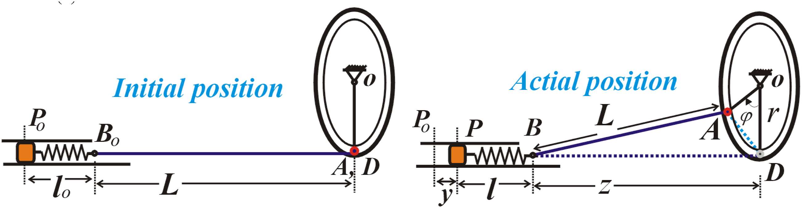
From the indicated Figure 1, it can be easily stated that:

let

The total force that affects the moving block is

The equation that controls the motion is known as:

Inserting Eqs. (1)-(3) in Eq. (4), it follows that the controlling dynamical equation of this system may be written as follows:

Using Taylor expansion, the righ hand side of ODE (5) can be approximately simplied under the condition

Within perturbation methods, quadratic terms can be expressed as various odd-order terms through operations such as multiplication, division, differentiation, and integration. The application of the NPA is primarily based on distinguishing odd functions generated by damping effects from those associated with stiffness nonlinearities. In this framework, quadratic components are introduced to represent both damping and stiffness forces. The first principal integral is employed to evaluate the equivalent damping, whereas the second is used to determine the equivalent frequency. The contribution of even-order terms may be incorporated into either the main integral or the alternative one, depending on the formulation adopted. The NPA methodology has been extensively developed and examined by El-Dib in a number of publications.29,30 Therefore, ODE as given in Eq. (5) can be expressed in the following form:


Figure 2 shows the curves given in Eq. 6, 7 in the part (a), and the curve of absolute error between them in part (b). (a) Illustrates a comparison for 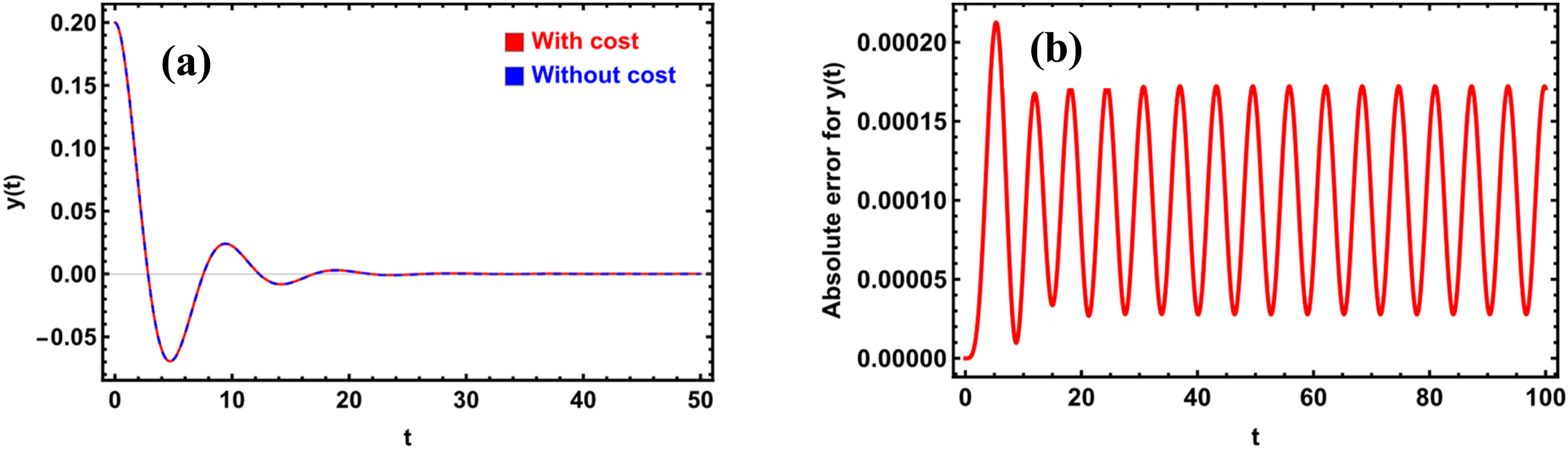
The guessing solution of Eq. (5) that satisfies the given ICs can be expressed as follows after the preceding NPA, see Moatimid et al.24–27:

The equivalent frequencies are evaluated using MS as follows
31
:

On the other hand, see Moatimid et al.,24–27 the equivalent damping term is given by

Therefore, the comparable linear ODE might be formulated as detailed below:

Figure 3 Illustrates a comparison for (a) Illustrates a comparison for 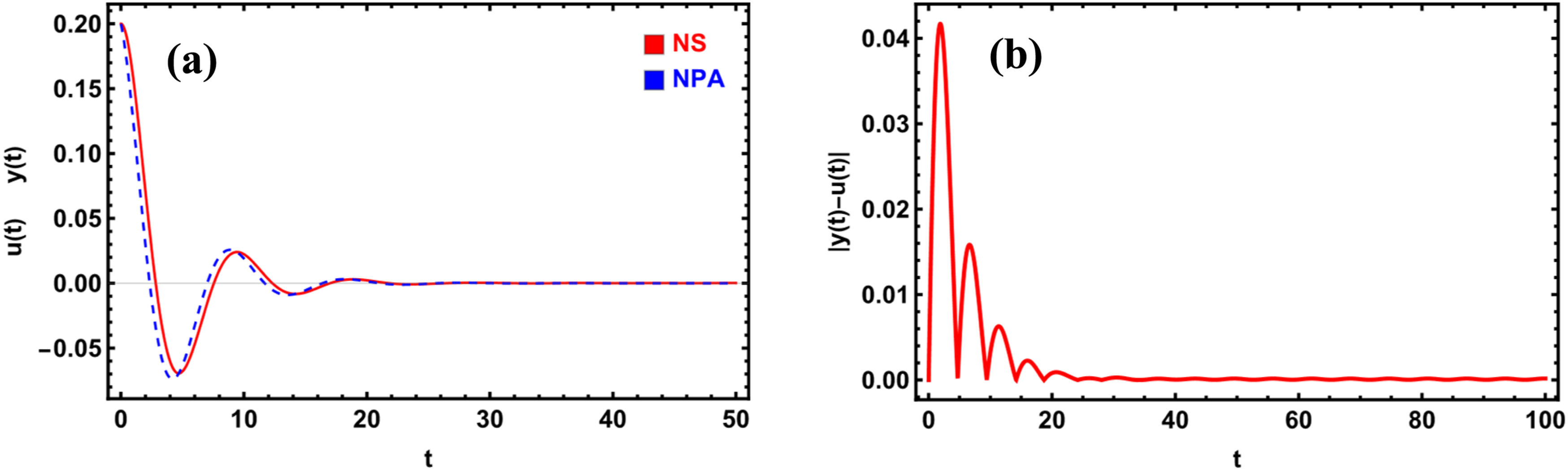
To remove the damping term

For an additional ease, the MS’s via the command NDSolve can be used to draw nonlinear ODE solutions as provided in Eq. (5) and their linear equivalent linear ODE as given in Eq. (10). For this motivation, suppose that the data are in the following given chosen sample:

Now, we are going to perform the achieved results in view of their graphical representations. The analysis of the first problem is presented throughout Figures 4–9. To ensure clarity, each figure contains no more than two parts. Let us break them down one by one: Shows the time-dependent solution Shows the time-dependent solution Presents the corresponding curves in the plane Presents the corresponding curves in the plane Demonstrates the stability areas according to condition (13) at the same values of the considered parameters in Fig. 4. Demonstrates the stability areas according to condition (13) at the same values of the considered parameters in Fig. 5.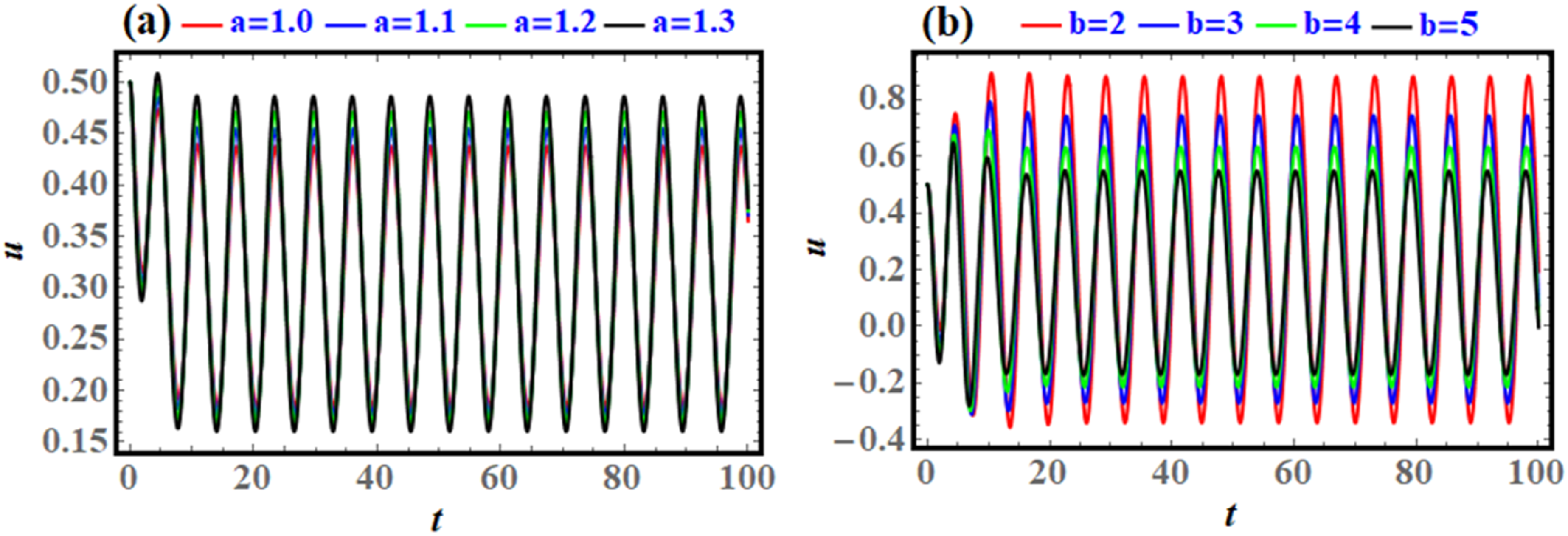
The solution’s response over time (displacement)
The related phase plane diagrams of the visualized curves are provided in Figure 6(a) and (b) and Figure 7. Figure 6(a) and (b) show the phase diagrams (velocity
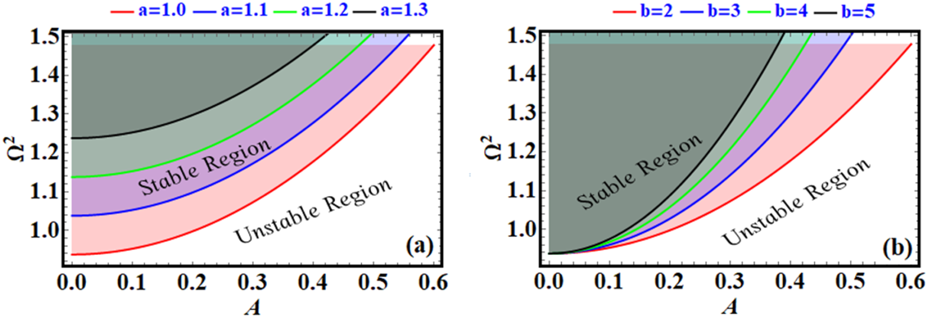
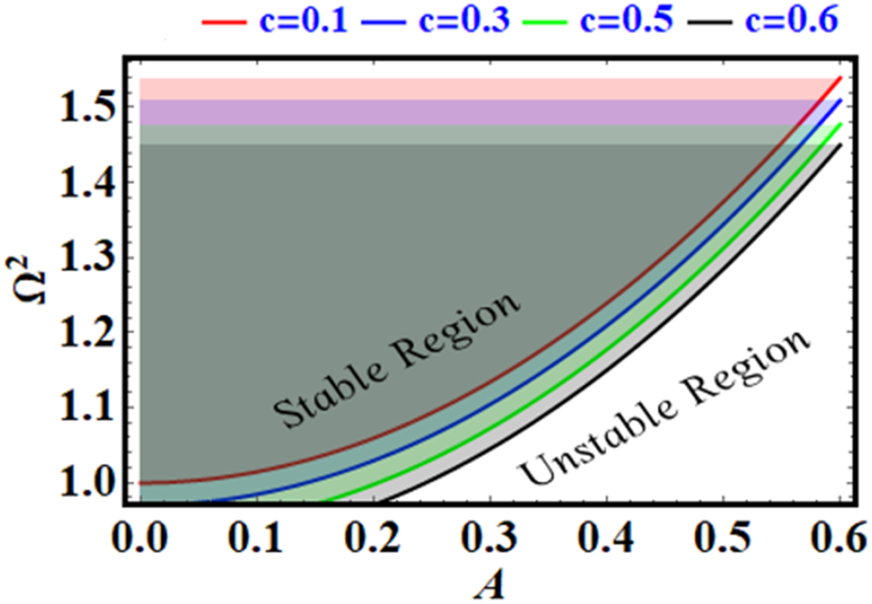
A closer look at the stability regions according to condition (13) is given in Figure 8(a) and (b) and Figure 9. Figure 8(a) and (b) display the stability regions as defined by the parameters
Overall, these figures collectively illustrate how parameters
2.1.1. Sensitivity analysis of bifurcations and chaotic dynamics to parameters
In this section, we analyze plotted figures that show how a system’s behavior changes as we adjust its settings. These graphs highlight the critical points where the system undergoes a major shift, revealing new stable states or periodic patterns. We also use PMs to gauge the system’s stability and potential for chaos. Together, these procedures reveal a deeper understanding of how complex systems evolve. 24 The “butterfly effect' is a famous way to describe chaos: minuscule changes at the start can completely alter the future, making it impossible to predict what will happen in the long run. 25 While the path a chaotic system takes seems random, it is actually following strict, deterministic rules, playing out within a complex, fractal-like shape known as a strange attractor.
We can measure this inherent unpredictability using LE. In simple terms, the LE calculates the average speed at which two nearly identical starting points will drift apart over time. A positive LE is indicative of chaos, indicating a constant divergence of trajectories. A negative LE, on the other hand, indicates stability and convergence.
25
Because of this, LE acts as a fundamental numeric signature for chaos, helping us to distinguish it from simple irregularity. Adjusting parameter
Figures 10 and 11 are calculated at Shows BD as Displays BD as 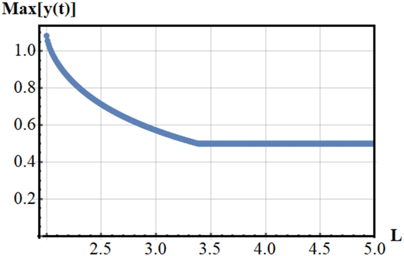
Based on these graphs, one can interpret this discussion physically as follows: Increasing
Both Figure 12 ( Displays BM for Shows PM for 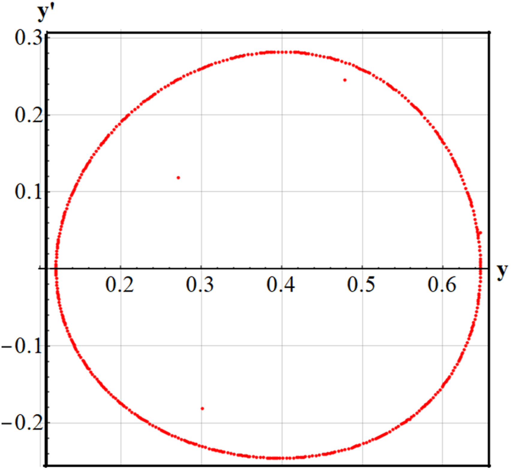
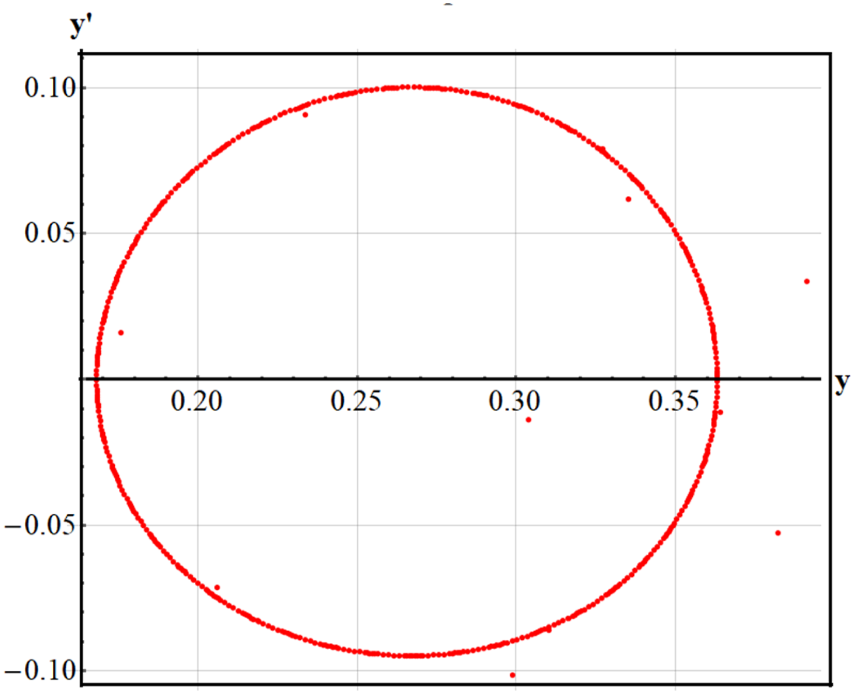
In Figure 13, the closed curve is much tighter and smaller, with fewer and less pronounced, energetic, and potentially slightly less regular oscillation pronounced outliers, demonstrating a more regular periodic motion with a smaller amplitude and reduced dynamical range, possibly indicating stronger damping or weaker forcing. Physically, one can state that the system with
Figure 14 at Shows the LEs when 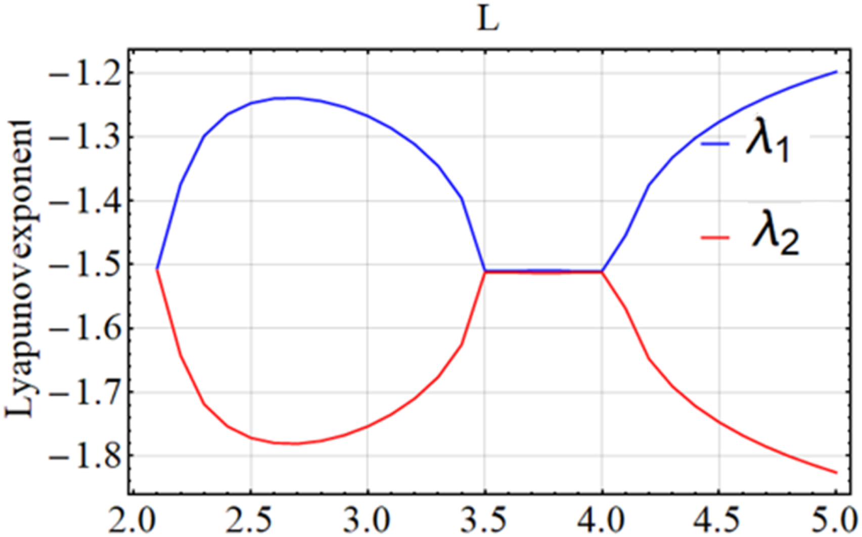
In Figure 15, both LEs are always negative and decrease only slightly. The higher exponent Displays the LEs when 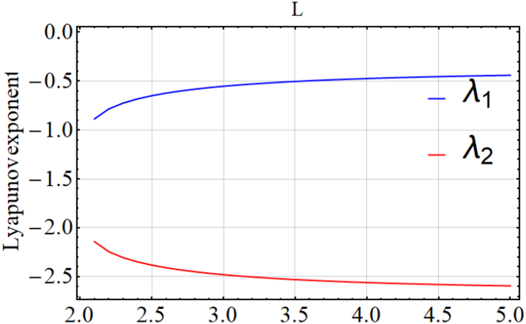
2.2. example 2
The second example involves a mass Displays a particle moving on a circular wire that rotates smoothly.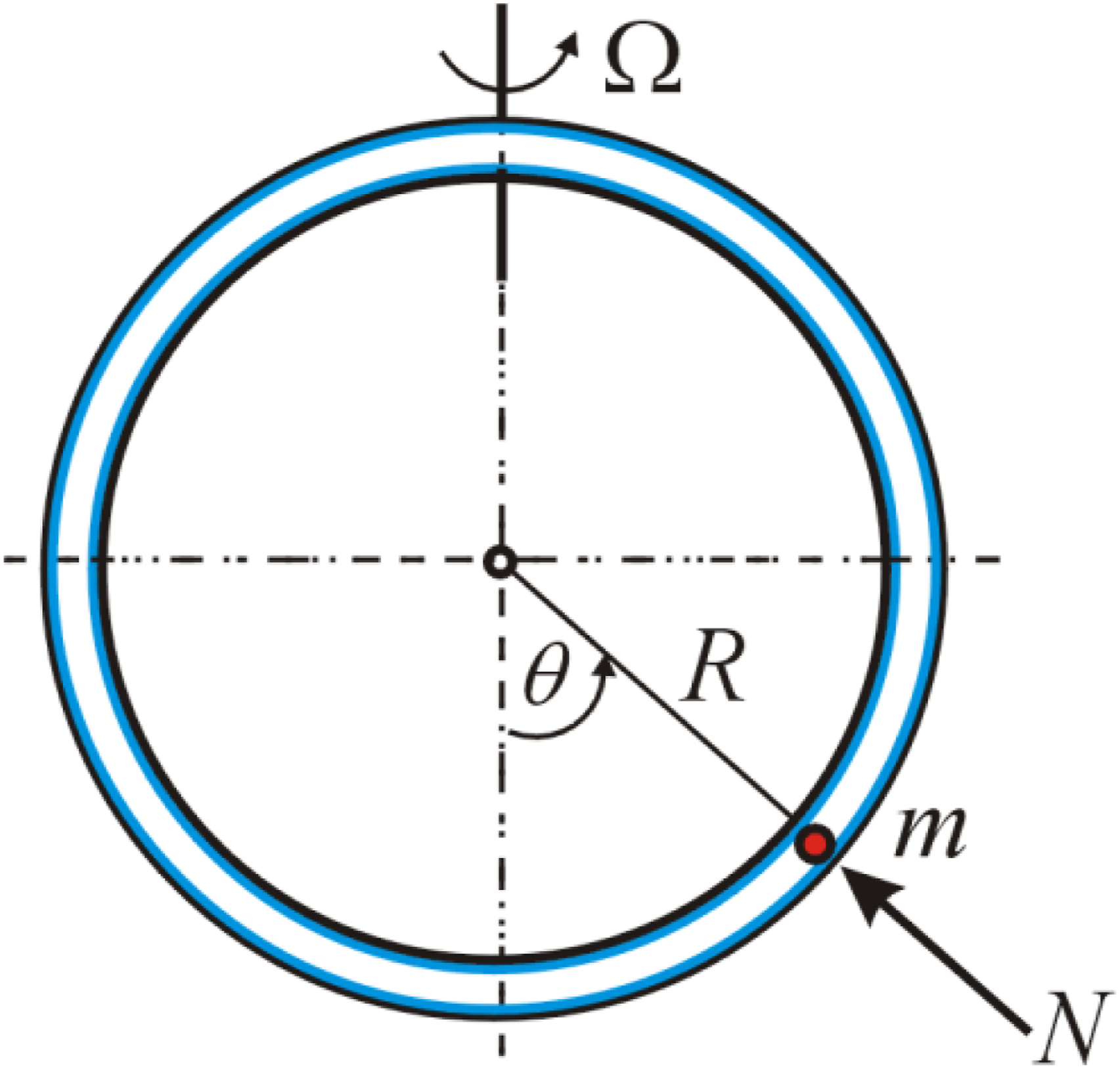
As previously shown,32,33 the kinetic component of the energy in the particle is T:

The gravitational potential becomes:
The potential energy from fictitious centrifugal force:
So, the total potential energy will be:

Formerly, the Lagrangian may be written as:

Applying Euler–Lagrange equation, one gets

Inserting Eq (16). in Eq. (17), the equation describing the motion is given by:

Dividing both sides over

The ICs is represented as:

Eq (19). can be stated as follows:

The initial solution may be represented as follows:

With similar ICs as given in Eqs. (20).
Because of the NPA’s benefit over all other conventional perturbation techniques, using Taylor expansion’s drawback is not necessary in this case.
As previously shown by Moatimid et al.24–27 and El-Dib,28–31 the equivalent frequency could be evaluated as follows:

Eq (23). can be rewritten as follows:

The stability criterion requires:

Accordingly, the equivalent linear equation may be represented as:

For more convenience, MS via command NDsolve to match the nonlinear ODE as given in Eq. (19) based on the linear comparative one as reflected in Eq. (26). Choose a sample system with the data:

A significant coincidence arises between two the plane curves of the oscillators, one described by a nonlinear ODE, as specified in Eq. (19), and the other following a linear form, as indicated in Eq. (26). This coincidence occurs when their trajectories in phase space or over time align evidently, despite their essentially distinct mathematical frameworks. The phenomenon appears under specific conditions where the impact of nonlinearity is negligible or sufficiently controlled by designated parameters, resulting in motion that closely resembles the linear case. Under specific conditions, the nonlinear system may display harmonic or nearly harmonic oscillations with frequency and amplitude attributes akin to those of its linear equivalent. This behaviour indicates a notable underlying symmetry within the nonlinear dynamics. The MS calculates the Absolute Error between the two solutions, yielding a value of 0.0440441 Figure 17.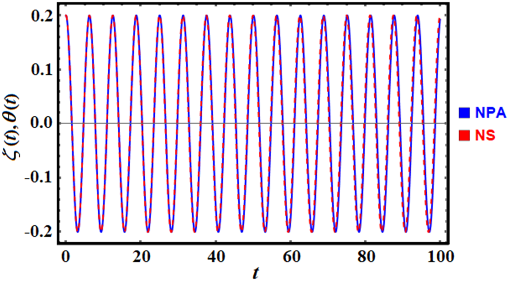
A plot of the absolute error, Shows absolute error 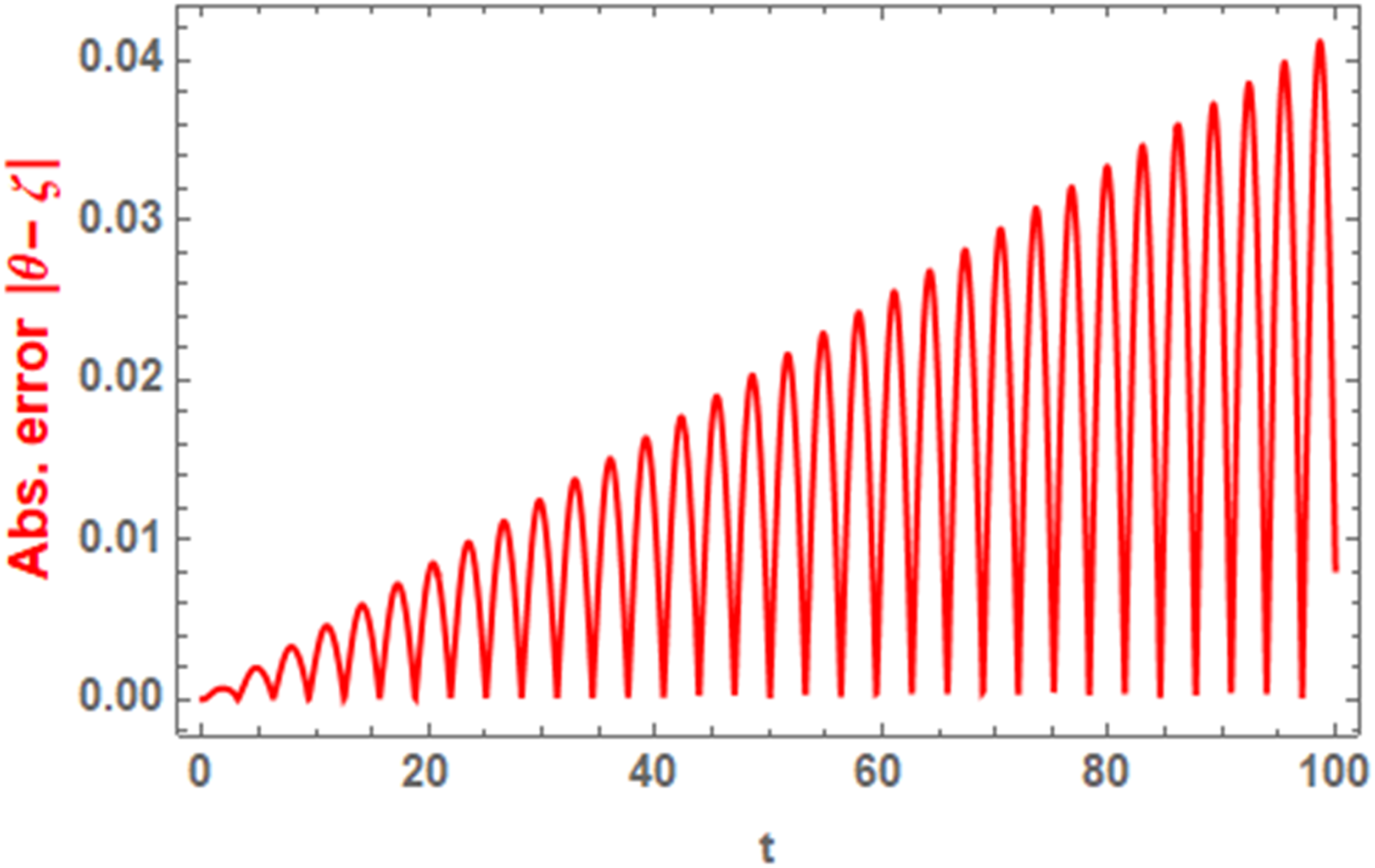
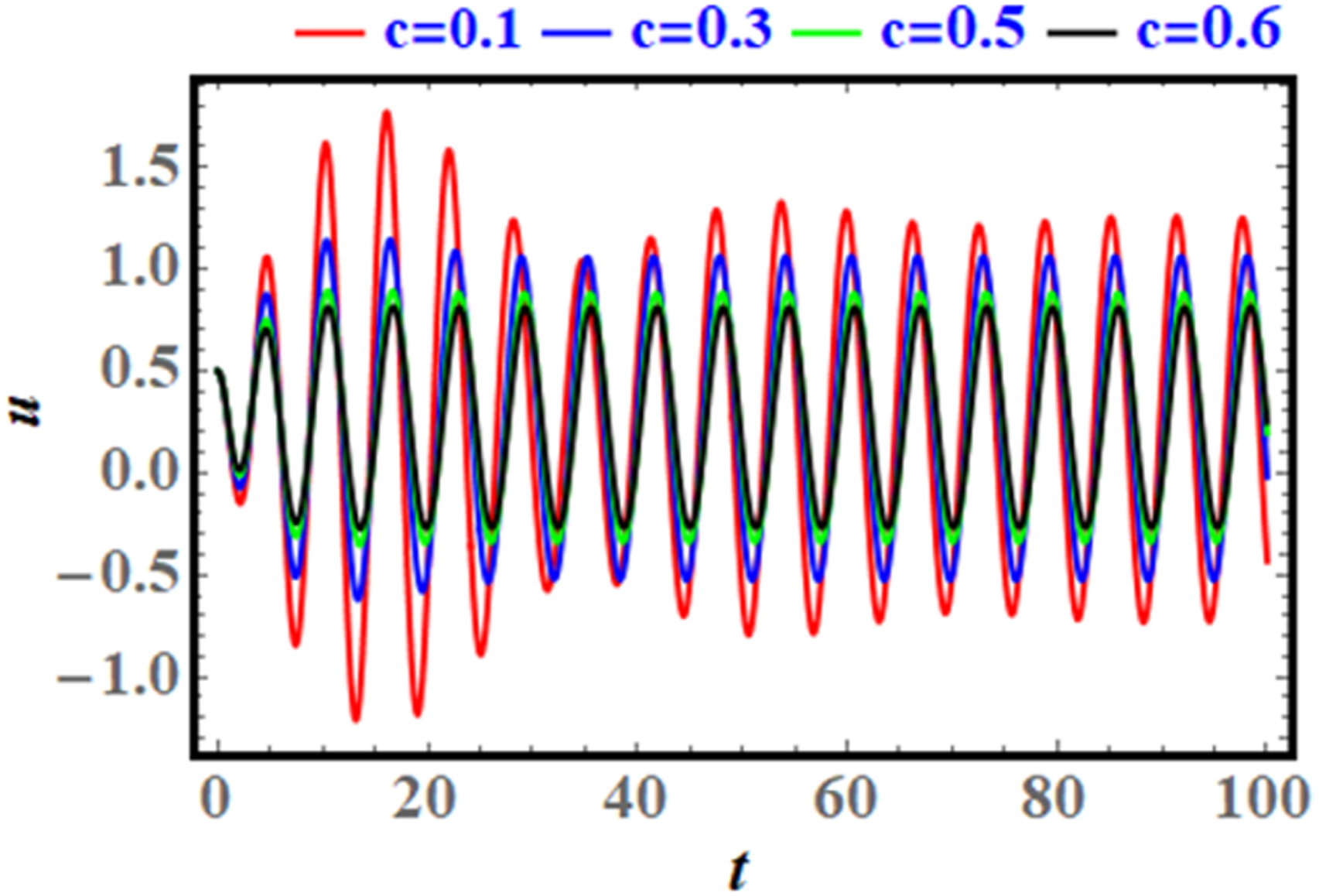
Here, we discuss the obtained results for the considered dynamical model in Example 2. Let us perform and interpret Figures 19–21 in the context referring to the movement of a mass Presents the behaviour of the solution 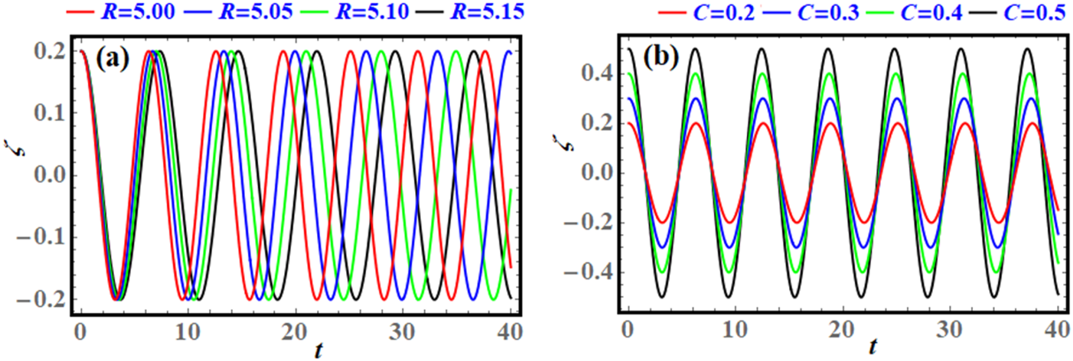
In view of the plotted curves in Figure 19, one can perform the panels (a) and (b), which express the time histories of
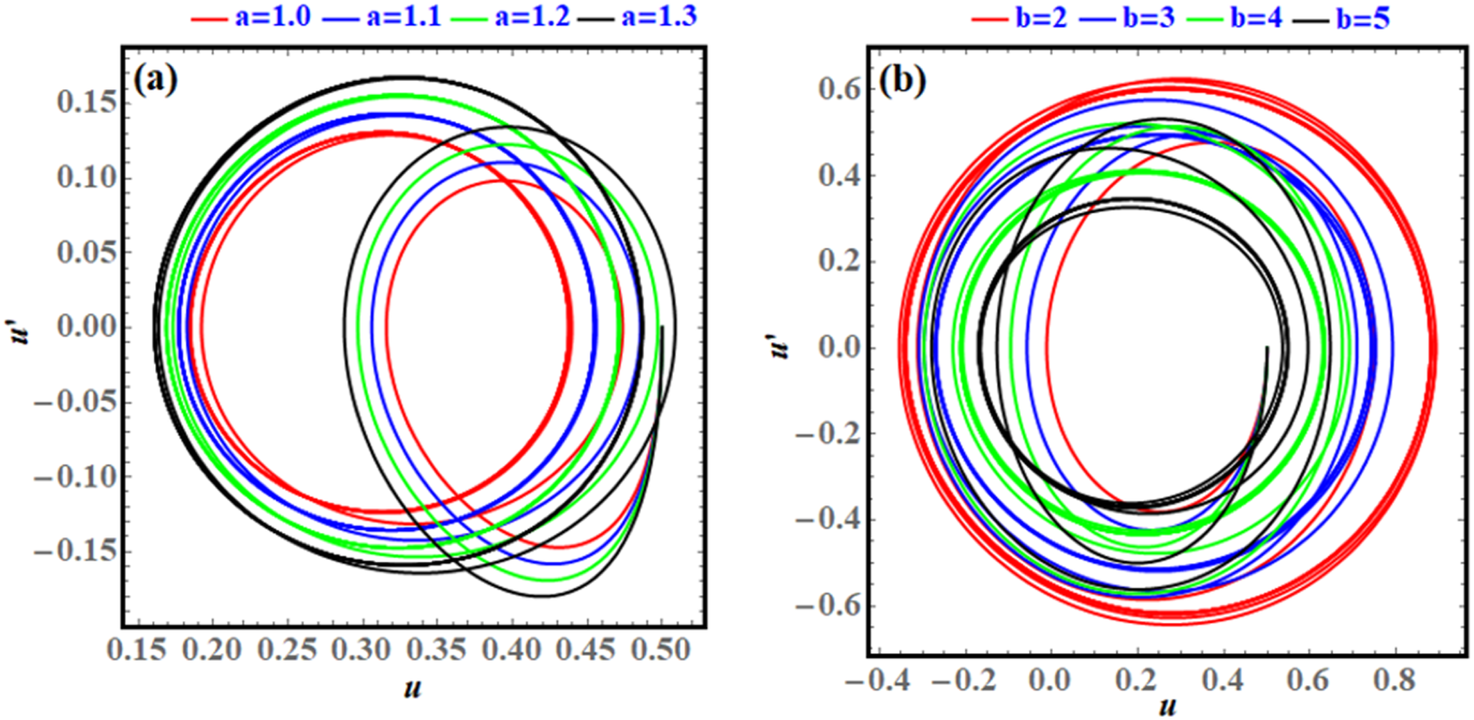
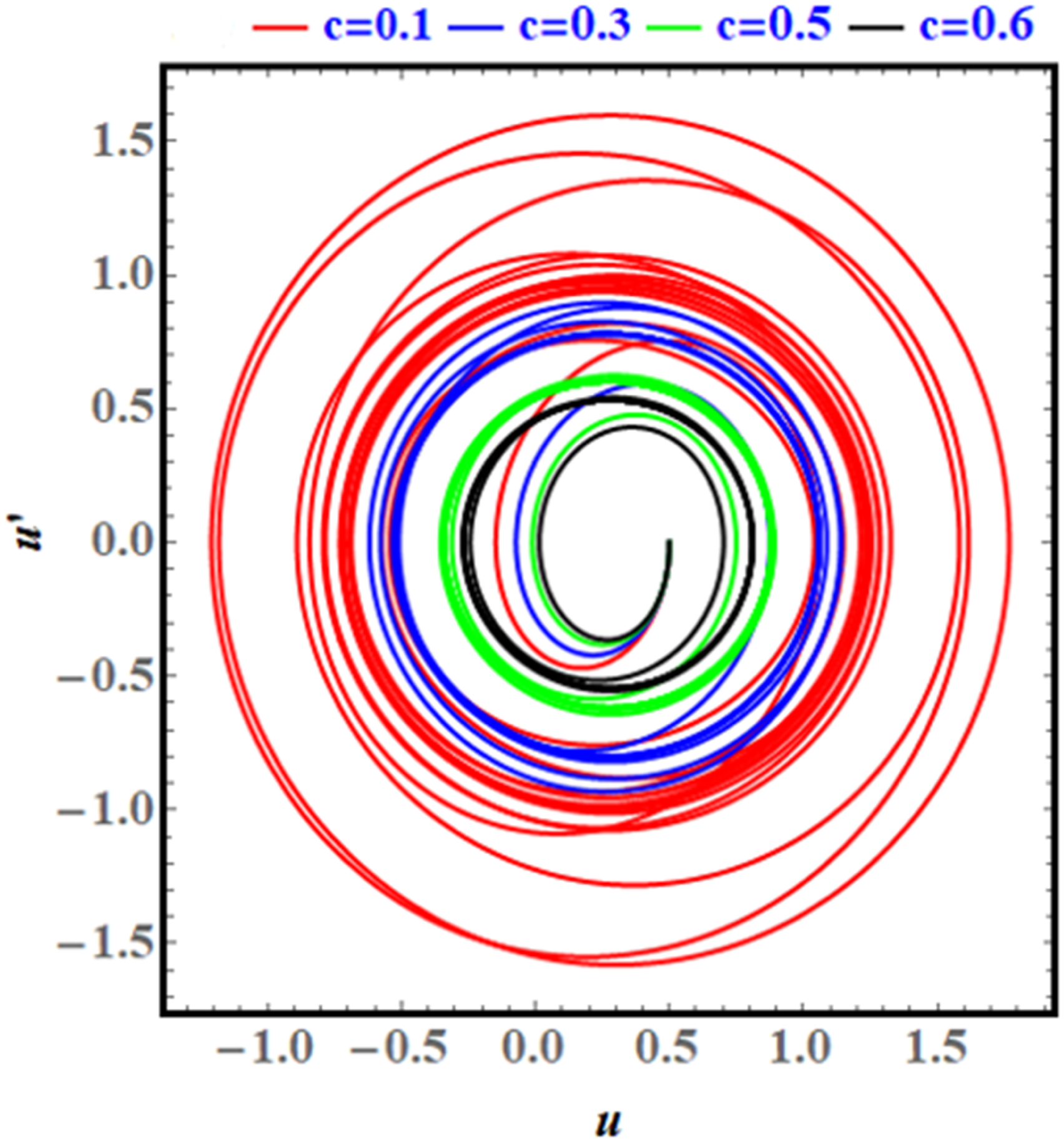
In Figure 20, panels (a) and (b) show how the phase portrait for this system plots ( Presents the behaviour of the phase plane plots at: (a) 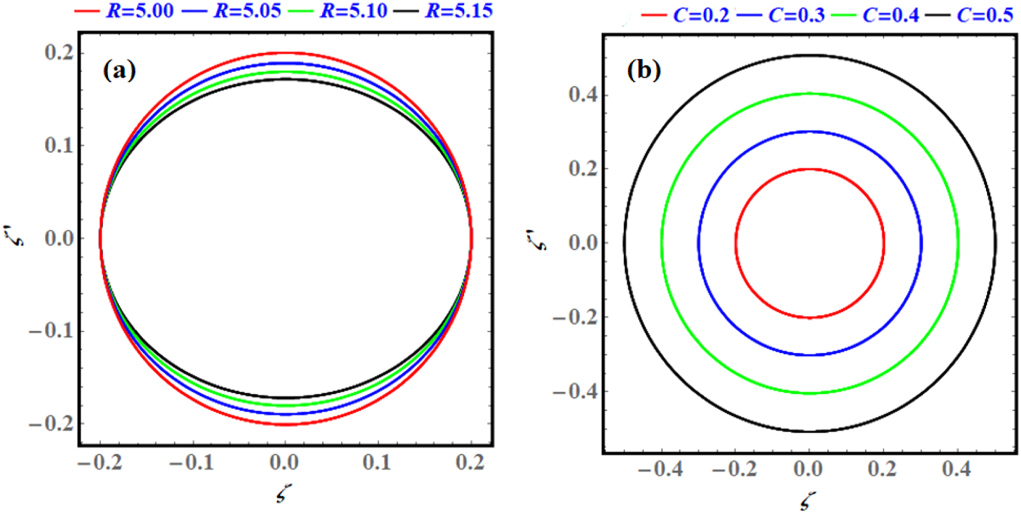
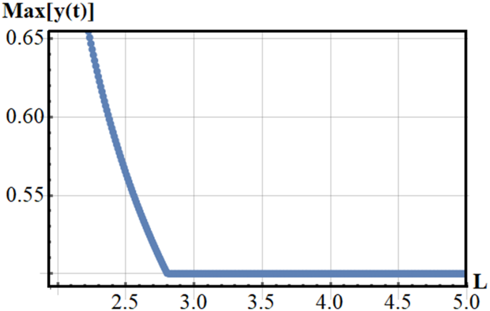
Analysis of the stability curves axes Illustrates the stability regions considering condition (25) at 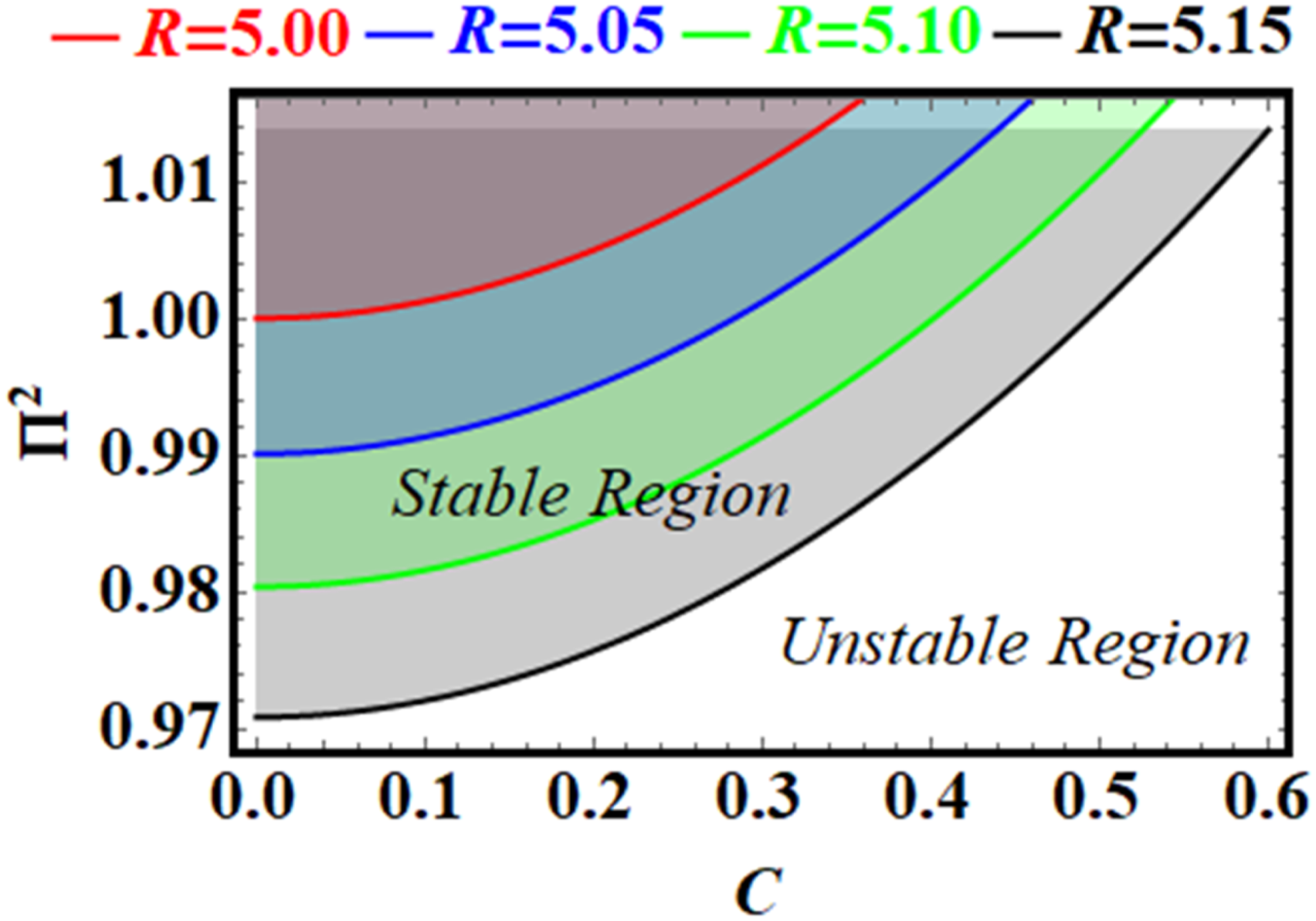
For larger
Generally, to keep the system stable, you need to manage the size of
2.2.1. Chaos and bifurcation analysis with parameter sensitivity
Here, we investigate how the system responds to changes in its parameters by analyzing a series of plots. These figures illustrate key transitions, such as the emergence of new steady states or periodic behavior. PMs are used to assess stability and detect signs of chaos, offering deeper insights into the evolution of complex systems.
Figure 22Figure 22 present the BDs illustrating the maximum angular displacement, Shows BM as Shows BM as 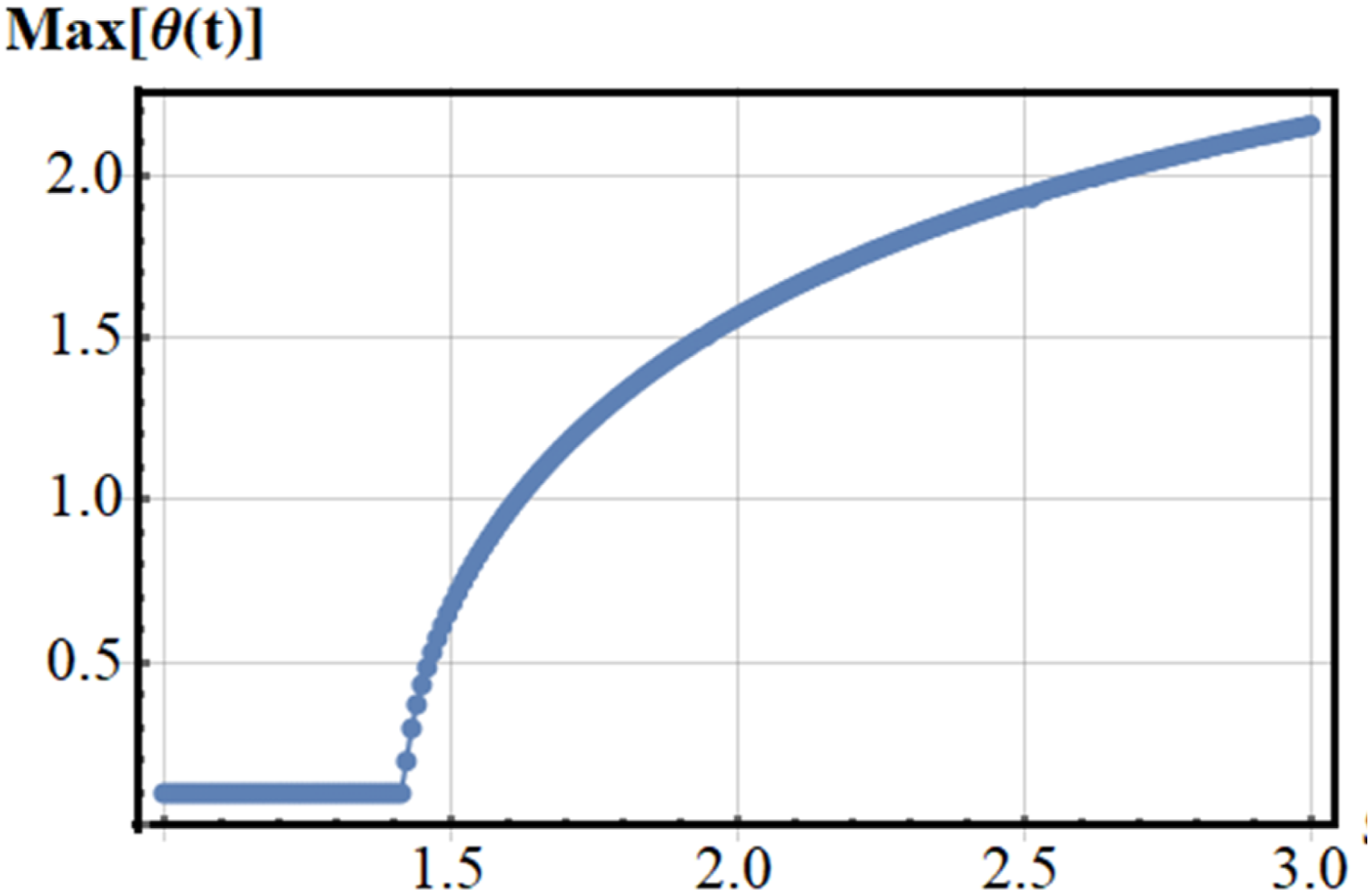
Based on the plotted graphs in Figure 22, one concludes that when
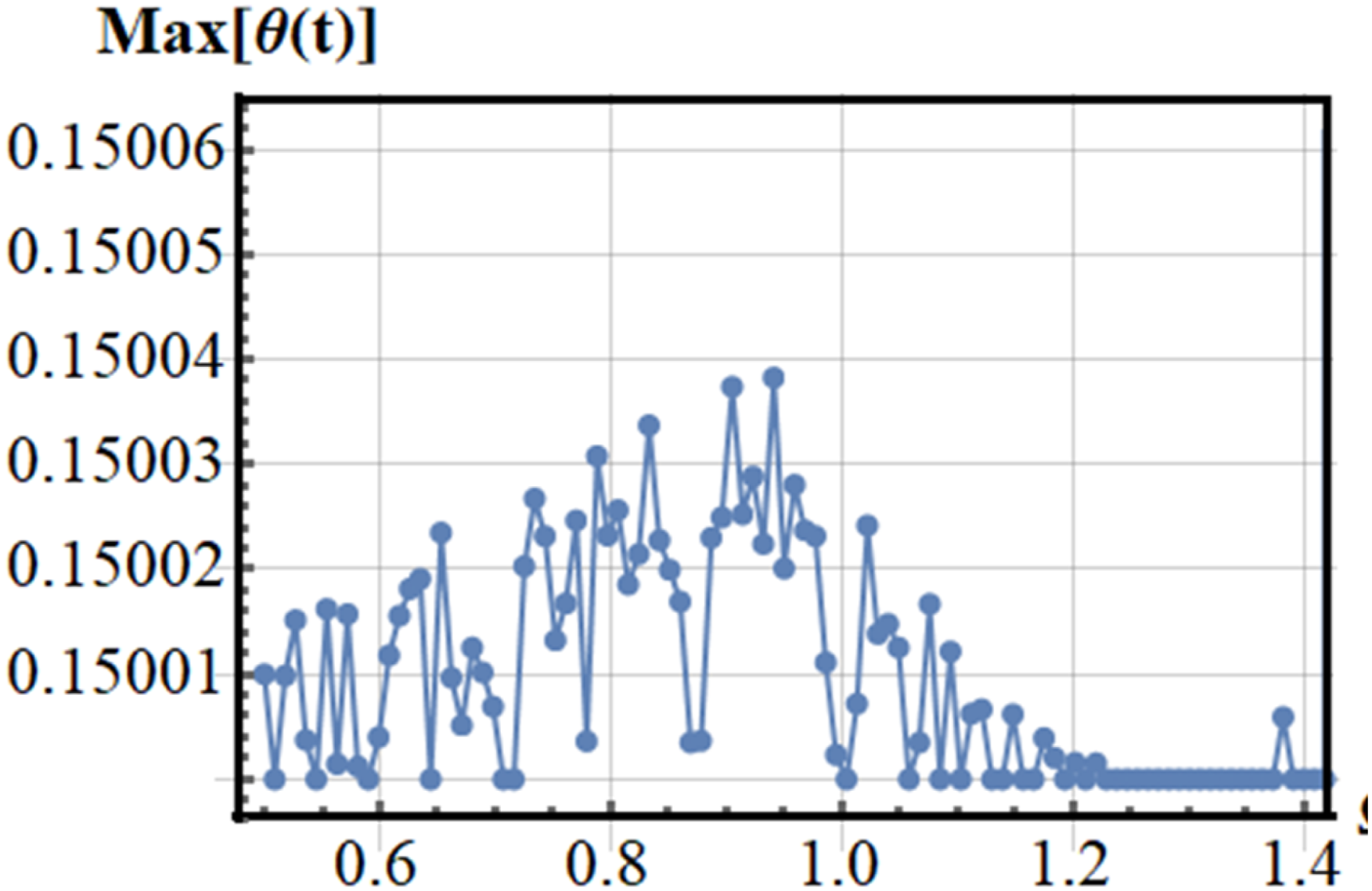
In contrast, Figure 23 is plotted, where a higher initial angle (
Shows a comparison of two Figures 22 and 23.
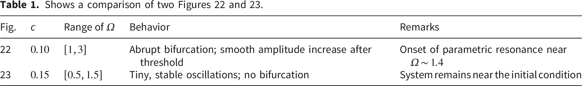
Figures 24 and 25 display PMs for two sets of parameters: Displays PM for Shows PM for 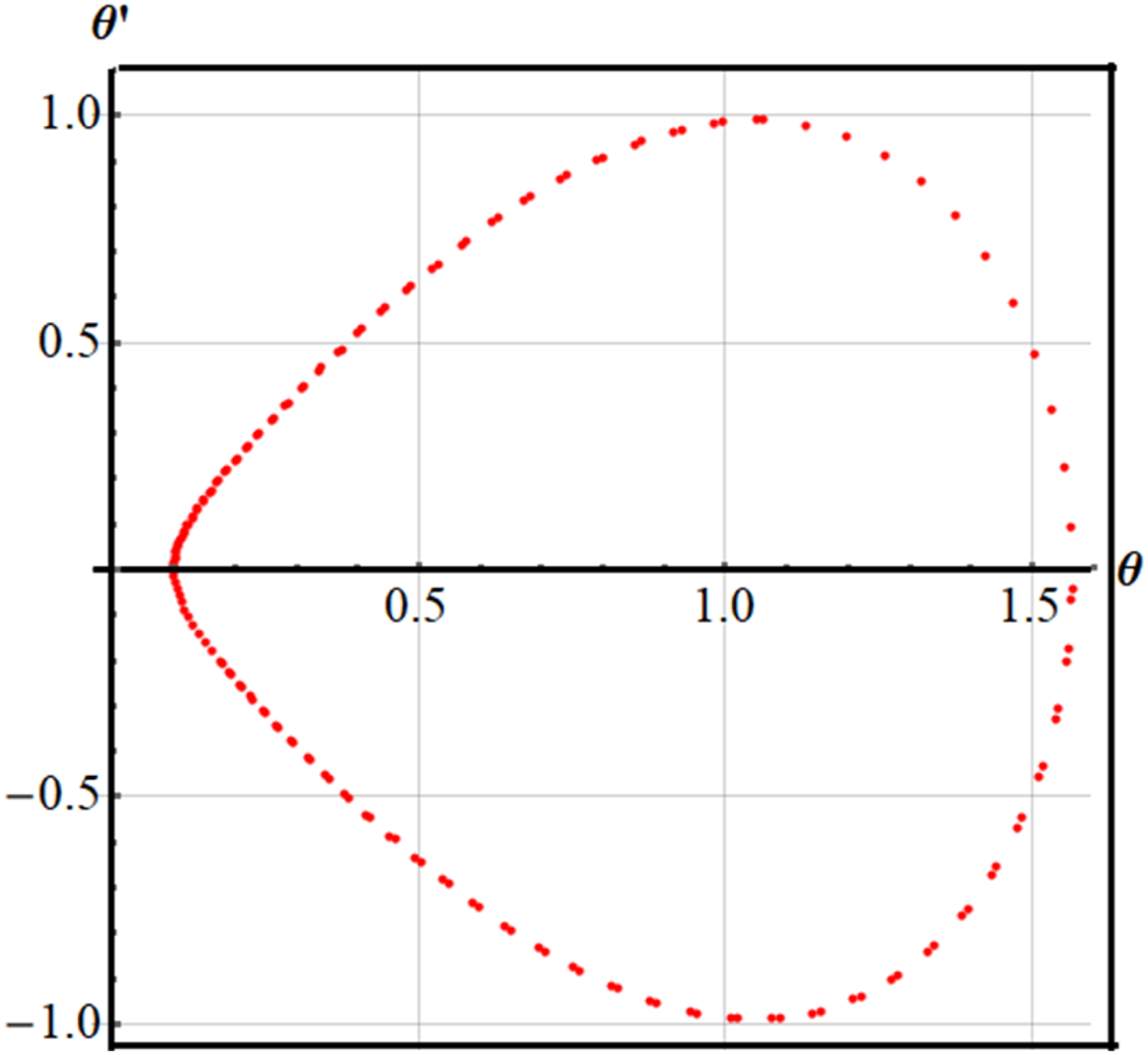
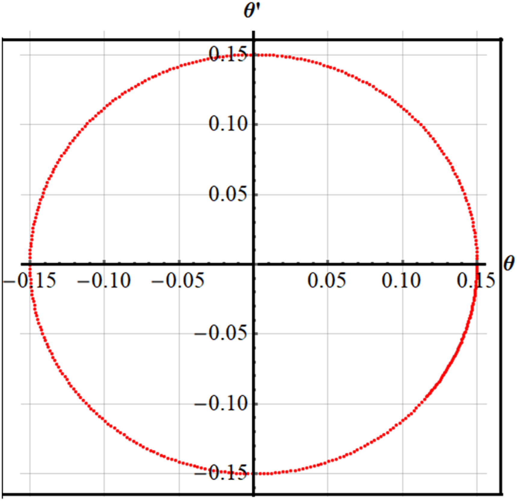
At
Shows a comparison of two Figures 23 and 24.
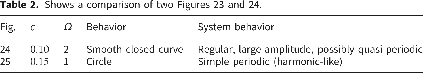
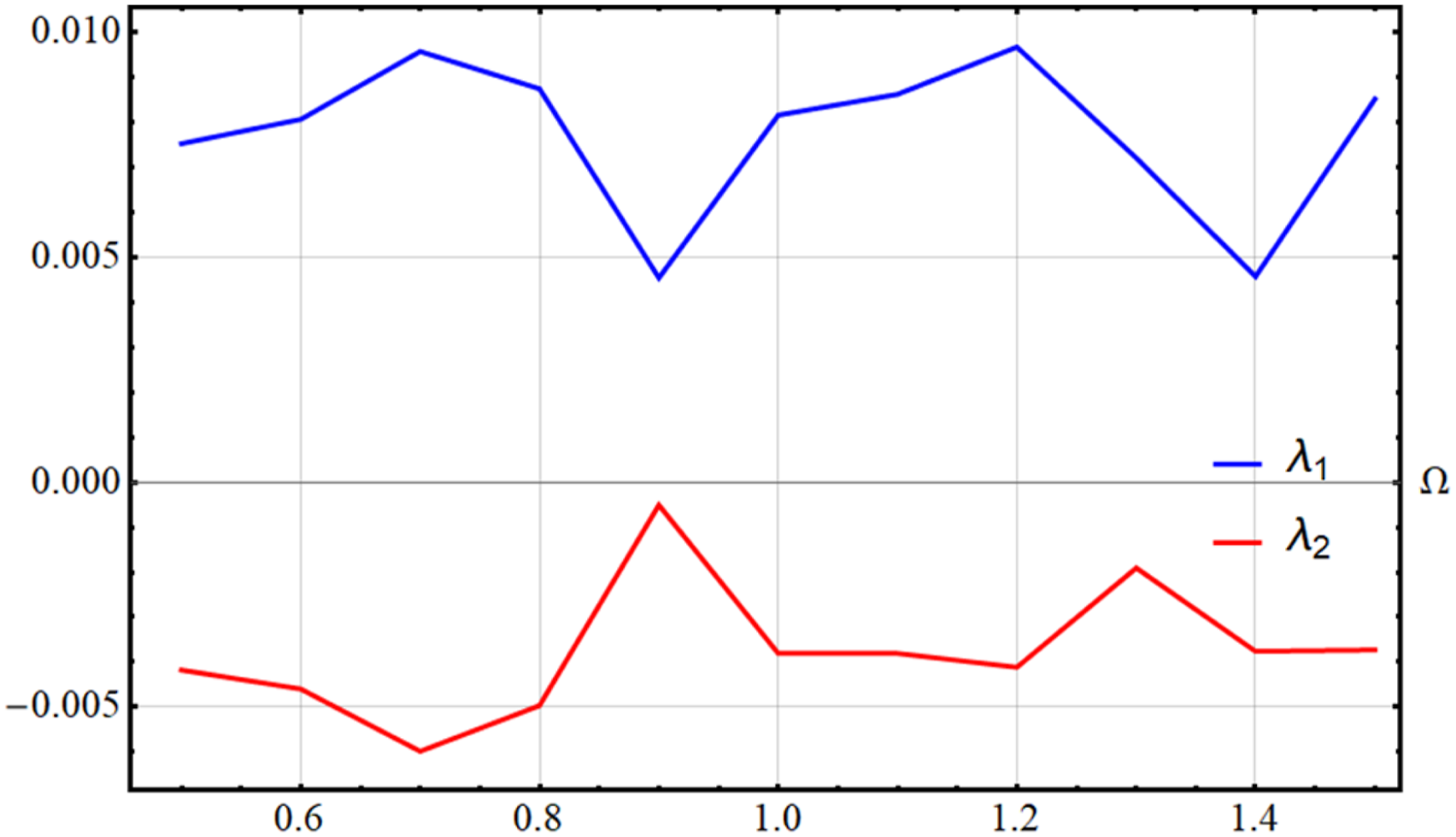
Figures 26 and 27 show the computed Lyapunov spectra for the rotating system as a function of the driving frequency Ω, with parameters Shows LEs when Shows LEs at 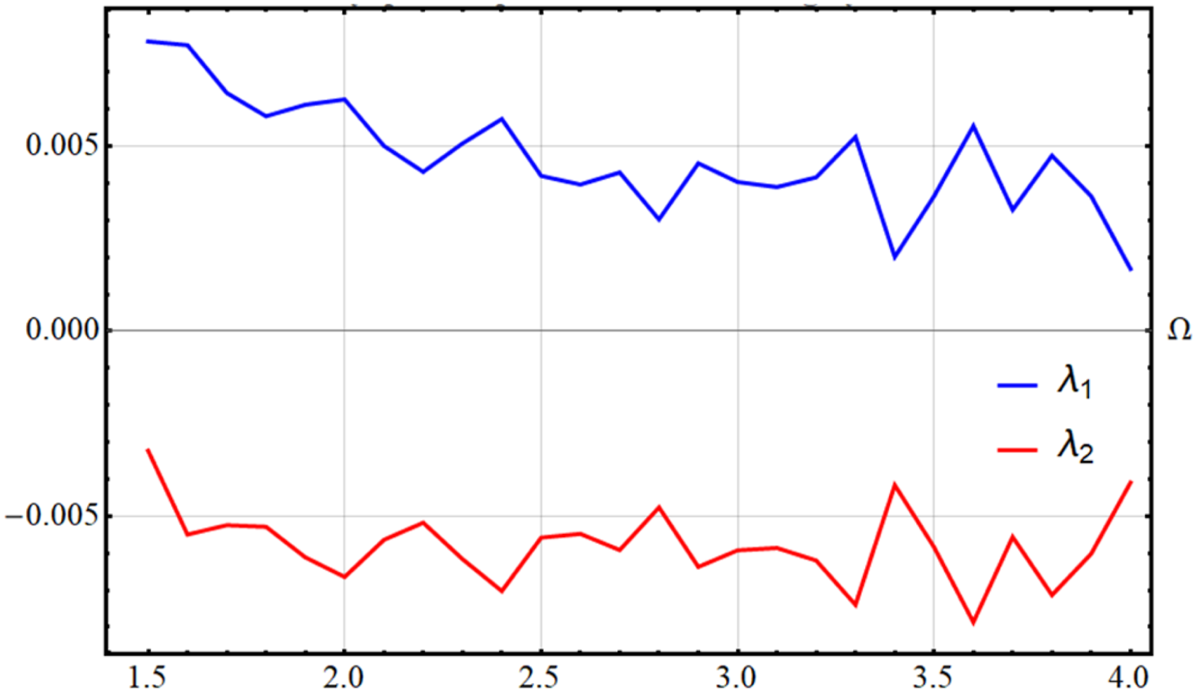
Based on Figure 26, we can write; the curves indicate the two largest LEs,
According to Figure 27, we can see that, for this parameter regime,
3. Concluding remarks
Nonlinear oscillations commonly manifest in real-world problems, including mechanical structures and biological cycles, leading to intricate behaviors such as bifurcations and chaos, which are essential in comprehending and forecasting dynamical systems. Progress in analytical and numerical techniques has facilitated innovative applications in engineering, medicine, and materials research. We examined oscillators exhibiting significant nonlinear characteristics, integrating both damping and restoring forces, through a combination of theoretical and computational methodologies. Two instances were provided from various scientific and technical domains. The novel methodology presented markedly decreases computing time and resource utilization relative to traditional perturbation methods commonly employed in this domain. Utilizing HFF, the suggested NPA converts a weakly nonlinear oscillator described by an ODE into a linear form, hence enabling the derivation of a new frequency associated with the linearized ODE. The theoretical conclusions were corroborated through NSs conducted via MS, demonstrating a strong correlation between the two ODEs. This approach enables a comprehensive examination of system stability, enhancing capabilities beyond those offered by prior methods. Accordingly, the NPA provides a more pragmatic and dependable framework through NSs of weakly nonlinear oscillators. Furthermore, it is distinguished as a versatile instrument for applied research and engineering owing to its adaptability to many nonlinear scenarios. We also analyze the influence of various parameters on stability, with results validating the approach’s simplicity, efficiency, and reliability. Modifying bifurcation parameters changes the configuration of BDs and their corresponding PMs, which we further demonstrated by mapping the LE curves. The principal key outcomes can be encapsulated as follows: 1. Two nonlinear oscillators governed by weak ODEs were analysed. 2. The stability study was conducted for each oscillator. 3. Dangerous operating zones characterized by unpredictable and unstable nonlinear oscillations are detected through chaos analysis. 4. The critical parameter thresholds that induce abrupt changes in system dynamics are determined using bifurcation analysis. 5. The LEs quantitatively assess stability and susceptibility to ICs.
Investigating linked weakly nonlinear oscillators is crucial as numerous physical and engineering systems comprise interacting components whose movement’s exhibit nonlinearity, particularly at moderate amplitudes. Weak nonlinearity engenders phenomena including amplitude-dependent frequencies, energy transfer across modes, synchronization, internal resonance, bifurcations, and the emergence of chaotic behavior, which linear theory alone cannot predict. Coupling enables oscillators to transfer energy and information, rendering these models crucial for comprehending vibrations in mechanical structures, electrical circuits, MEMS and NEMS devices, aeronautical systems, rotating machinery, biological rhythms, laser dynamics, and power grids. Analyzing coupled weakly nonlinear oscillators from an engineering standpoint facilitates the design of stable and efficient systems, the control of undesirable vibrations and resonance, the enhancement of signal processing and communication technologies, the improvement of energy harvesting devices, and the prediction of failure mechanisms in complex interconnected systems.
Footnotes
Acknowledgments
The Researchers would like to thank the Deanship of Graduate Studies and Scientific Research at Qassim University (www.qu.edu.sa) for financial support (QU-APC-2026).
Author contributions
Funding
The Researchers would like to thank the Deanship of Graduate Studies and Scientific Research at Qassim University (www.qu.edu.sa) forfinancial support (QU-APC-2026).
Declaration of conflicting interests
The authors declared no potential conflicts of interest with respect to the research, authorship, and/or publication of this article.
Data Availability Statement
This study was not supported by any data.