Variation of shock-spacing during screech stage-jumps

Abstract

Flow visualization is used to investigate shock-spacings in a supersonic jet during stage-jumps associated with the screech phenomenon. Conventional schlieren and shadowgraphy techniques as well as a new projection focusing schlieren technique are employed. Both time-averaged and instantaneous snapshots of the flow field are analyzed for a 37.6 mm round convergent nozzle over the jet Mach number range of 1.0 < M_j < 1.7. Shock-spacing is studied especially during hysteresis of the stage-jumps where two different screech frequencies could be realized at exactly the same M_j depending on whether the latter variable was increased or decreased. The data follow a monotonic trend without any discontinuity at any M_j. This establishes the fact that the stage-jumps in frequency are not associated with abrupt changes in the shock-spacing.

Keywords

screech stage-jump hysteresis supersonic jets shadowgraphy flow visualization

Introduction

Supersonic jets at imperfectly expanded conditions, characterized by a train of shock cell structure, often produce a sharp tone known as screech. Powell¹ first studied screech tones and offered an explanation for the underlying mechanism. In essence, a small disturbance starts in the initial shear layer near the nozzle lip and grows as it propagates downstream. When amplified sufficiently, it interacts with the shock cells in the jet plume to produce sound. The sound propagates upstream to the nozzle lip to generate embryonic disturbances and thus the feedback loop is closed. The process is accompanied by the generation of an intense tone referred to as screech. The phenomenon has since been studied by numerous researchers that advanced and refined our understanding of it; Raman² provides a comprehensive review of past work. We now know that the disturbance growth occurs due to the instability characteristics of the jet’s shear layer.^3–5 The noise is produced by the interaction of the amplified instability wave (manifesting as coherent vortical structure) with the train of shocks downstream.^6–9 The noise-producing shocks (typically the 3rd to 5th from the nozzle) undergo small-amplitude perturbation over the screech period about their mean position.¹⁰ There is some evidence that the noise may be produced by a “whip-lash”-type motion of the tips of the shocks, that extend into the shear layer, as a coherent vortical structure passes through (invited talk by R Westley 1997, see Raman,² also noted during presentation of Edgington-Mitchell et al.¹¹). Compared to the small periodic motion of the shocks the flow field goes through much larger amplitude unsteady motion.

A curious “stage-jump” process occurs with screech frequency variation. With increasing jet Mach number (M_j) the frequency decreases in a stage until there is a sudden jump to the next stage involving a higher or lower frequency. The frequency again keeps decreasing with further increase in M_j until a jump to another stage takes place. The stage-jump usually displays hysteresis, i.e. the jump occurs at either higher or lower M_j depending on whether the latter variable is increased or decreased. For a round jet, at least five stages, labeled A₁, A₂, B, C, and D, are usually encountered.^1–3,12,13 The measured nondimensional frequencies in various stages may not be exactly the same from experiment to experiment but are sufficiently close for such identifications.^2,3 The different stages are known to involve different “modes” of flow field oscillations.^2,7,14–16 Thus, stages A₁ and A₂ are known to involve axisymmetric modes while stage C is characterized by a helical mode. Stages B and D typically include flapping mode oscillation. A flapping mode may be considered as the superposition of equal amounts of left and right helical modes. The direction of flapping may not be fixed and it may undergo a precession that is unpredictable even in a given experimental set up. The B and D stages may be unstable, switching between the flapping and helical modes. It is noteworthy that the staging behavior has also been observed in numerical simulations.^4,17 However, the stage-jump (sometimes also referred to as mode-jump) is one aspect of screech whose mechanism has remained far from being clearly understood, as discussed further in the following.

There have been many analyses for prediction of screech frequency. Starting with Powell’s original analysis, all such predictions require shock-spacing as an input parameter. In fact, with any given analysis screech wavenumber and frequency are uniquely determined by the shock-spacing. Analytical prediction of shock-spacing has also been pursued in several past works. Pradtl originally provided an analysis that was further modified by Pack.¹⁸ Further analyses were provided in Tam et al.¹⁹ and Morris et al.²⁰ All of these provide a first approximation of shock cell spacing as a function of the nozzle pressure ratio (or, jet Mach number, M_j). With all other variables remaining constant shock-spacing, and hence screech frequency, is therefore predicted as a continuous function of M_j. Here lies a glaring deficiency in the knowledge of screech. None of the analyses so far can handle a stage-jump that is a discontinuous function of M_j. As stated in Raman,² “despite numerous papers on the topic, no one to date has offered clear explanation for the mode jumps”.

Keeping in mind that there have been many sophisticated measurements and analyses on the subject, we keep our goal limited in this study. We take a step back and ask a simple question: does the shock-spacing undergo a sudden jump to accommodate a new frequency (wavelength) when a stage-jump takes place? To the best of the author’s knowledge, this obvious question has not been directly addressed before. One may ask: is it even reasonable to expect abrupt changes in shock spacing as M_j is varied? As stated before, all available analyses assume shock-spacing to be a continuous function of M_j. Experimentally, however, small perturbations at the lip of a given nozzle are known to affect shock structure. Use of vortex generators (tabs) has been shown to drastically alter shock structure as well as their spacing.²¹ Thus, it is not implausible that shock-spacing goes through an abrupt adjustment during screech stage-jumps. This is what we explore in this study. It is needless to say that pertinent knowledge of the issue is important for understanding and modeling of not only screech but also other components of shock associated noise from supersonic jets.

Earlier, we had conducted an experiment using background oriented schlieren (BOS) technique for measuring shock-spacing.²² However, while BOS has its merits (e.g. hardware simplicity) it is not as effective in discerning precise shock boundaries due to limited spatial resolution. Thus, in order to address the issue at hand further we decided to revert back to conventional schlieren and shadowgraphy techniques and repeat the experiment. The latter techniques have their own drawbacks. There is spatial and temporal averaging that might obscure small variations in shock-spacing. Mindful of this, we first make a comparative assessment of several techniques while analyzing time-averaged, instantaneous and focused flow fields. Data on shock-spacing from all techniques are then studied with special attention given to regions of hysteresis associated with the stage-jumps. These results are presented in the following.

Experimental setup and procedure

The study was conducted in an open jet facility at NASA Glenn Research Center. Compressed air, supplied through one end of a 760 mm diameter plenum, exited through a 37.6 mm diameter convergent nozzle on the other end.¹³ The flow discharged into the quiescent ambient of the test chamber and all data pertained to unheated flow acquired over a range of 1.0 < M_j < 1.7. The facility is used mainly for flow field measurements. However, the ceiling and side walls of the chamber have acoustic linings and with proper precaution qualitative noise measurements are also possible. Here, we are concerned primarily with the frequencies of the screech tones for which the setup is considered adequate. Some further comments are made later about the quality of the screech frequency data.

A z-type configuration was used to implement schlieren and shadowgraphy techniques.^23,24 A top-view diagram is shown in Figure 1 with relevant dimensions. For time-averaged and instantaneous data acquisition it was necessary to use different light sources. The “interchangeable light source” in Figure 1 was coupled to a fiber and a 0.55 mm diameter fiber face served as the extended light source for the system. A continuous white light source and a pulsed cyan LED were used for the time-averaged and instantaneous measurements, respectively. Light rays indicated by solid (green) lines illuminated the spherical mirror on the left that collimated the light through the flow field and onto the spherical mirror on the right. The latter refocused the light to form an inverted image of the source. A knife edge was placed at the focal point when acquiring schlieren data. A Nikon 135 mm lens equipped with a Nikon 2× teleconverter imaged the test region onto a camera detector. The teleconverter was used in an effort to maximize the resolution. The scientific-grade CCD camera had a detector consisting of 4008 × 2672 pixels. For time-averaged schlieren and shadowgraph data, 12-bit images were captured with a 25 ms exposure time. For “instantaneous” snapshots, the 5 W 505 nm LED, pulsed at 1 µs, was used as the light source. The LED was pulsed using a controller which enabled precise control of the current to facilitate stable and repeatable illumination. By inserting the knife edge, it was possible to acquire instantaneous schlieren data using the above setup. Note that the time-averaged schlieren and shadowgraphy and instantaneous shadowgraphy used the same z-type setup and, therefore, all techniques resulted in images with identical fields of view and spatial resolutions of approximately 20 cm and 0.079 mm/pixel, respectively.

Figure 1.

Top view schematic of the z-type configuration used to acquire schlieren and shadowgraphy data.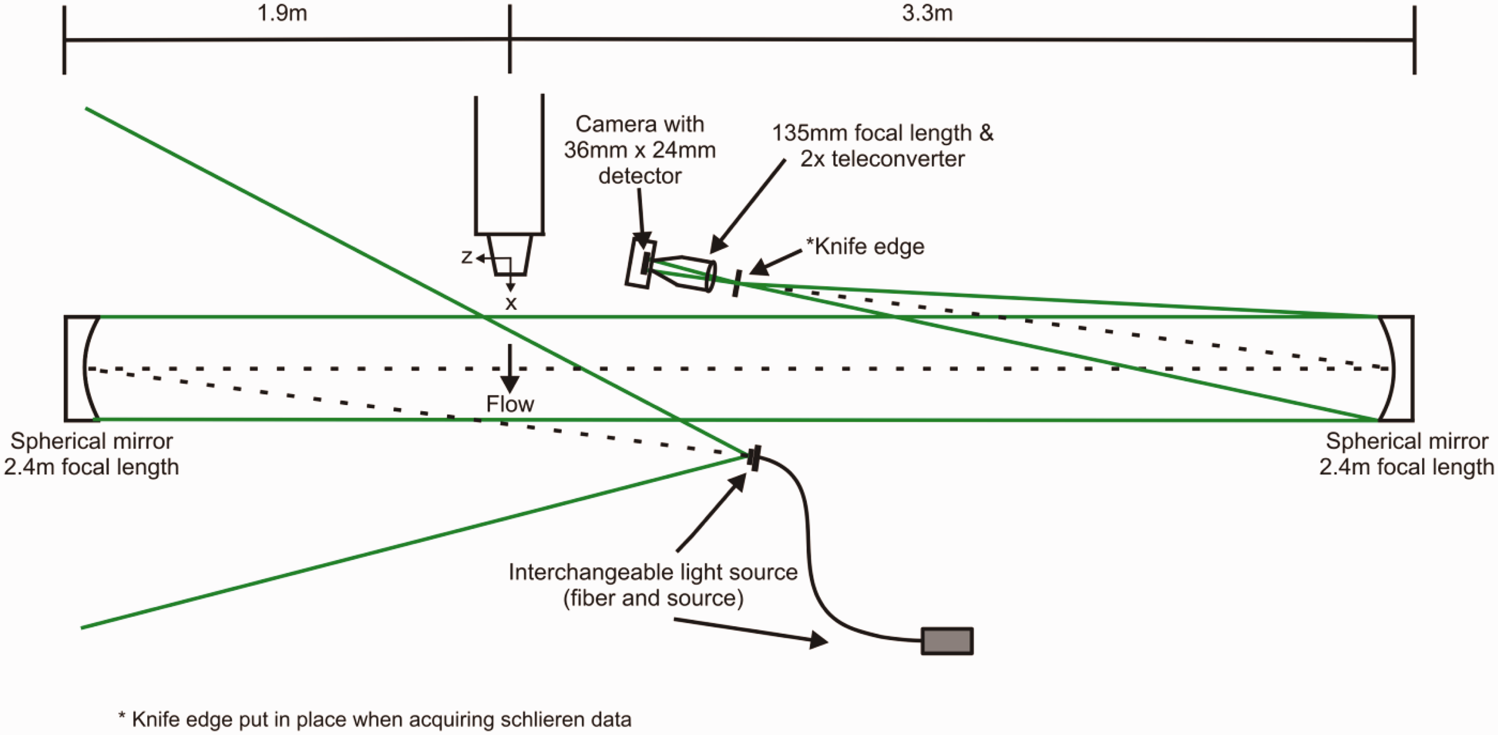

A dual projection focusing schlieren system, developed through NASA’s Small Business Innovation Research Program, was used to acquire instantaneous focusing schlieren data. A 5 W xenon flash lamp with 1 µs pulse duration was used to capture instantaneous snapshots of the flow. A series of lenses projected an image of the source grid onto a screen and a set of identical lenses re-imaged the projected grid onto a cut-off grid. An image of the flow field was captured onto the 4032 × 2688 pixel detector of a scientific-grade CCD camera located behind the cut-off grid. The resulting 8-bit images had a spatial resolution of 0.0624 mm/pixel. All optical components as well as the CCD camera were securely housed in a 58 cm × 43 cm × 25 cm case, which was placed on one side of the jet while a 76 cm × 61 cm retro-reflective screen was placed on the other side. The distances of the case and screen from the jet’s center plane dictated the size of the field of view. The chosen distances, within the constraints of the test chamber, provided a field of view that extended approximately 23 cm in the streamwise direction. The thickness of the focused field was estimated to be about 8 cm. Further details can be found in Weinstein²⁵ and Fagan et al.²⁶

Results and discussion

Assessment of the flow visualization techniques for measuring shock-spacing

Figure 2(a) to (d) shows examples of time-averaged shadowgraph, instantaneous shadowgraph, time-averaged schlieren, and instantaneous focusing schlieren images at M_j = 1.11. It can be seen that the flow and shock boundaries are most clearly defined in the time-averaged shadowgraph and time-averaged schlieren images (Figure 2(a) and (c)). The turbulent flow structures captured in the instantaneous snapshots of Figure 2(b) and (d) obscure the shock boundaries making it difficult to identify the shock cell tips (used to measure the shock-spacing). Comparing only the time-averaged data, the tips of the shock cells in the shadowgraph image (Figure 2(a)) appear sharper and more “point-like” than the corresponding tips in the schlieren image (Figure 2(c)). In addition, details are lost between the shock cells due to the dark regions of the time-averaged schlieren image, therefore the time-averaged shadowgraph is deemed more favorable compared to its schlieren counterpart.

Figure 2.

Sample images acquired at M_j = 1.11 using various flow visualization techniques.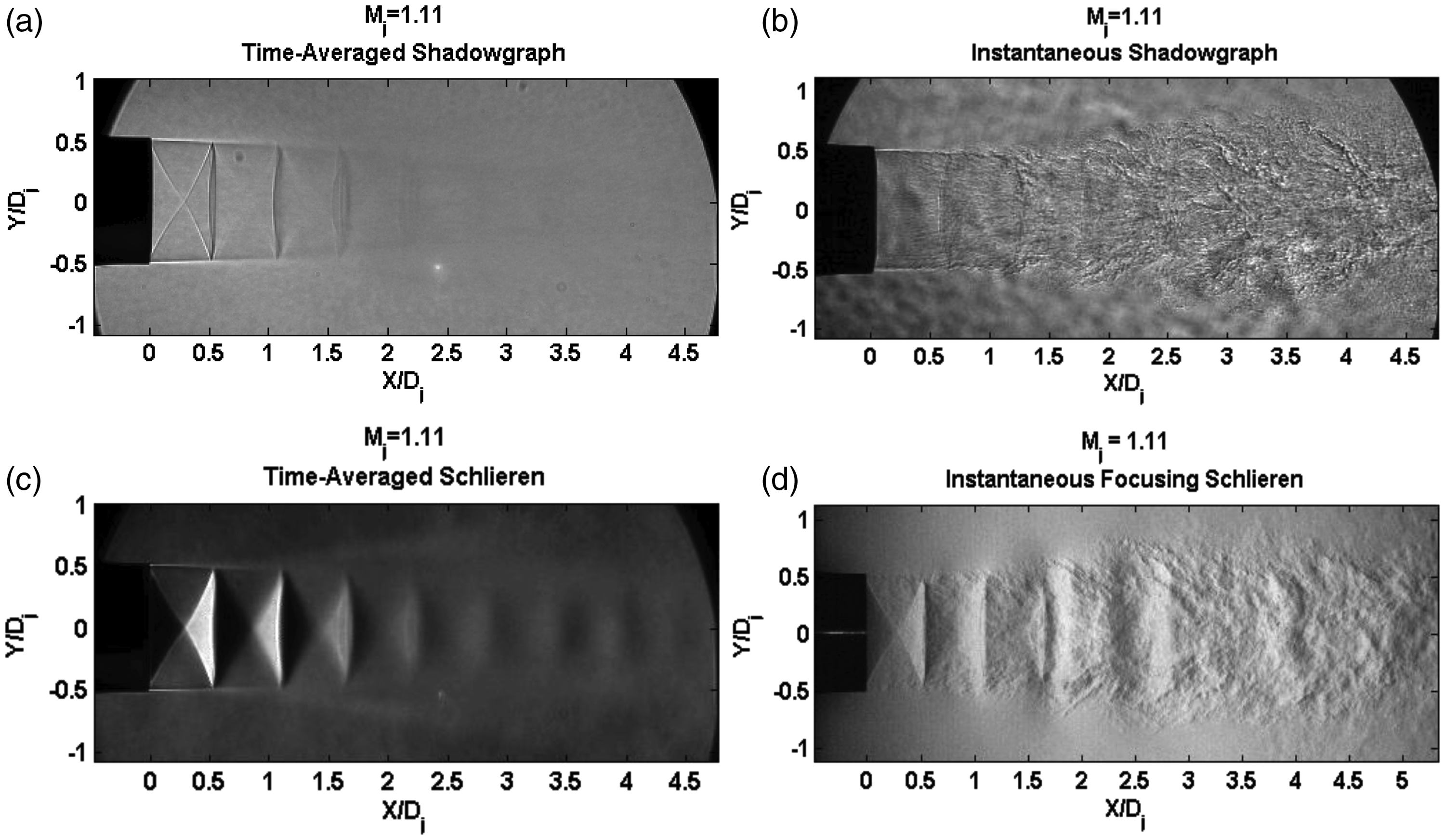

Due to the highly unsteady behavior of the screech stage-jump, instantaneous data were examined to determine if large oscillations of the shock-spacing took place. With both shadowgraph and focusing schlieren 10 instantaneous snapshots for given cases were studied. The shock cells within each ensemble did not reveal any abrupt movements beyond the techniques’ uncertainty. This provided the confidence that the time-averaged data did not wash out significant details. Thus, time-averaged shadowgraph was used as the primary method for further examination of shock cell spacing even though results from all other techniques are included for determination of the overall trend.

Shock cell spacing was determined as follows. Two representative time-averaged shadowgraph pictures are shown in Figure 3(a) and (b) for M_j = 1.04 and M_j = 1.24, respectively. The tips of the shocks at the jet’s shear layer are marked by the square symbols. When the shock is seen to start from inside the nozzle, an average of the first two tip-to-tip distances is taken to be the shock-spacing, as is the case in Figure 3(a). When the shock is seen to start at the nozzle exit, a third tip-to-tip spacing is measured, as shown in Figure 3(b). The averaging is deemed justified because the spacing is not expected to change within the first two to three cells while an average provides a better representative value. At a given M_j, the data were obtained from a set of three images and the average value was recorded. The process was repeated for each M_j. Assuming a Gaussian distribution,²⁷ the uncertainty of the mean with a 95% confidence interval is used in the shock-spacing estimates at each M_j. Note that due to the low number of samples (N = 3) the Student’s t-value for 2 degrees of freedom is used to calculate the uncertainty.²⁷ These results are discussed in the next subsection.

Figure 3.

Method for shock-spacing determination: (a) average of first two tip-to-tip spacings for M_j = 1.04 and (b) average of first three tip-to-tip spacings for M_j = 1.24.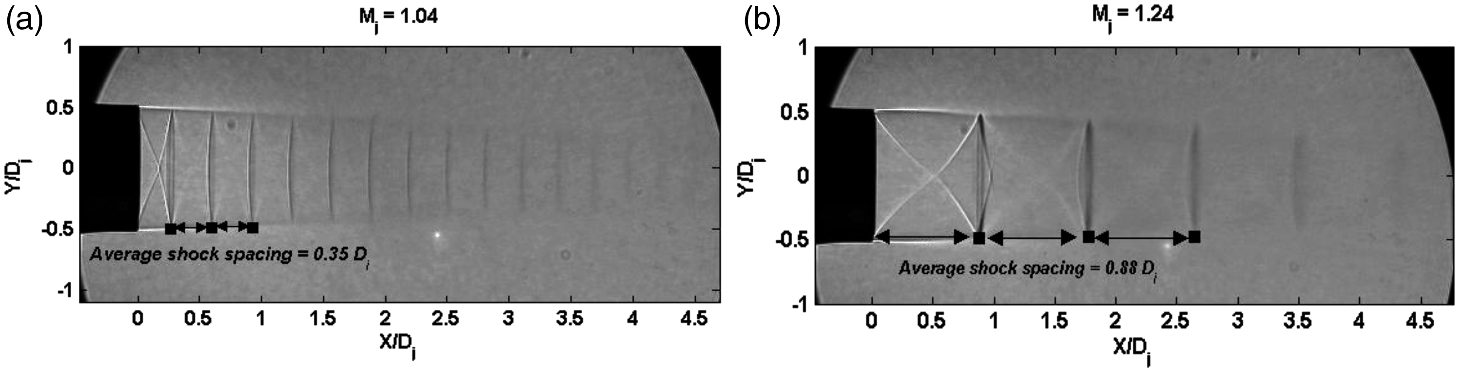

Results

Screech frequency data were acquired by spectrum analysis of the acoustic signal from a microphone positioned at 25° relative to the jet axis; (data at 90° showed the same trend, 25° data were chosen because they involved a stronger fundamental and fewer harmonics). Figure 4 shows the screech frequencies plotted versus M_j. As discussed in the introduction, the frequency within a given stage is seen to decrease continuously as M_j is increased. Stages A₁ and A₂ (axisymmetric), B and D (flapping), and C (helical) have been noted in most previous studies. Additional stages, not usually reported before, are observed here. These are labeled as B′, E, and F. While additional stages beyond D have been noted in some previous works, stage B′ appeared anomalous. Since screech frequency is sensitive to reflective surfaces, spot-checks were made with and without acoustic treatment of nearby surfaces. For the acoustic treatment, foam material was wrapped over the flange of the plenum chamber as well as other hard surfaces nearby. This did not alter the frequency data of Figure 4; stage B′ repeated faithfully. Thus, it is likely that differences in the lip and the interior of the nozzle as well as the nozzle’s outer geometry immediately upstream of the lip might play a role in producing these minor differences from experiment to experiment. However, these issues are of little concern for the problem at hand. The fact the stages were repeatable was adequate for the purposes of this study. With exactly the same hardware configuration, the frequency and the shock-spacing data were acquired for varying M_j. Note that there are clear overlaps between stages C and D, D and E as well as E and F. In each of these overlap regions of hysteresis, data could be obtained at exactly the same M_j but with different frequencies of different stages.

Figure 4.

Fundamental screech frequency versus M_j.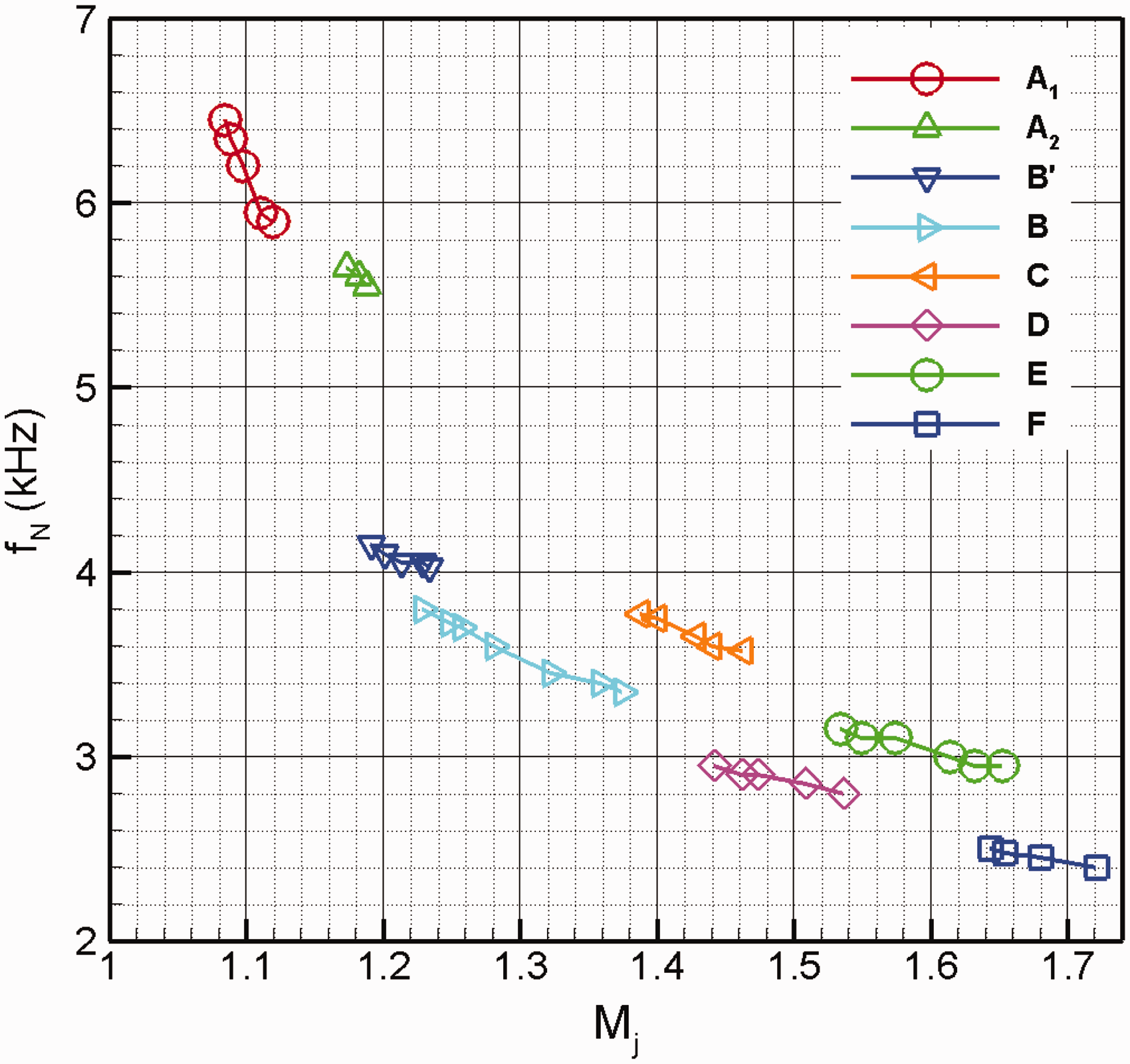

Examples of sound pressure level spectra in the hysteresis regions are shown in Figure 5 (the same color codes are used for the spectral traces as for the symbols in Figure 4). The suffix “U” in the legend indicates that the spectra were recorded as M_j was increased, while suffix “D” is used for the case when M_j was decreased. Figure 5(a) to (c) shows spectra pairs acquired at the nominal values of M_j = 1.46, 1.53, and 1.65, respectively. In each case, the emitted screech tone occurred at two different frequencies depending on whether the target M_j was approached from a lower or higher value. The hysteresis phenomenon is clearly captured by these pairs of spectral traces.

Figure 5.

Sound pressure level spectra during stage-jumps involving hysteresis: (a) stages C and D, (b) D and E, and (c) E and F. Suffix “U” in legend denotes data recorded when M_j was increased to target value and “D” when M_j was decreased to target value.

Both time-averaged and instantaneous flow visualization data were acquired for conditions corresponding to the different data points of Figures 4 and 5. Representative time-averaged shadowgraph images are displayed in Figure 6(a) to (l). Figure 6(a) shows an image without any perceptible screech tones present. Figure 6(b) to (f) shows images for screech stages, A₁, A₂, B′, B′ + B, and B, respectively. Figure 6(g) to (l) shows hysteresis pairs (Figure 5) where the adjacent stages could be captured at the same M_j for stages (C, D), (D, E), and (E, F), respectively. Inspection of Figure 6(g) to (l) right away indicates that there are no peculiar changes in the shock structure during the stage jumps. The shock structure and spacing appear identical for each of the three pairs.

Figure 6.

Time-averaged shadowgraph images at different M_j: (a) without any perceptible screech, (b) stage A₁, (c) A₂, (d) B′, (e) B′ + B, (f) B, (g,h) C and D stages within hysteresis loop, (i,j), D and E stages within hysteresis loop, (k,l) E and F stages within hysteresis loop.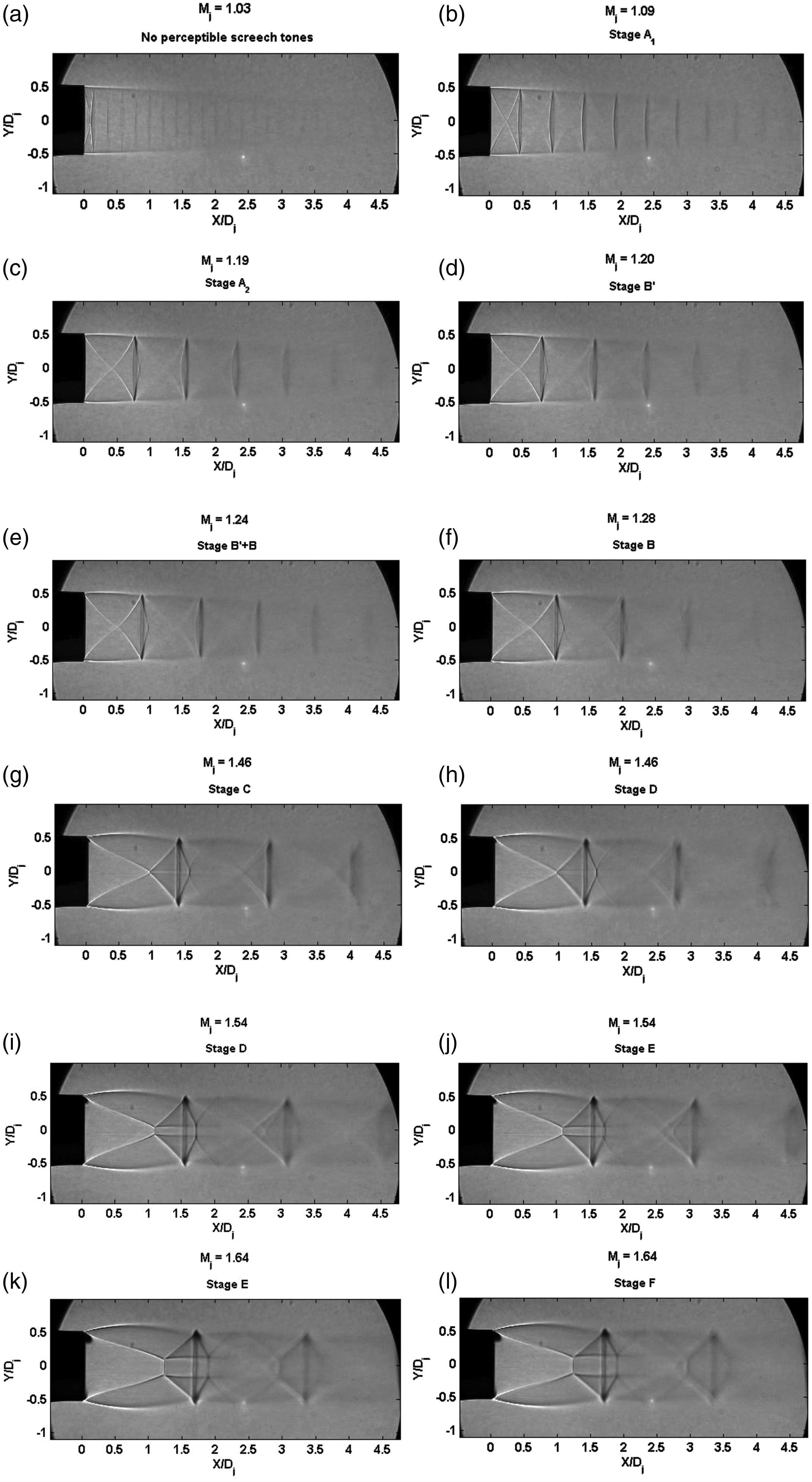

The shock-spacing was determined in the manner described in “Results and discussion” section and the resulting nondimensional values are plotted in Figure 7 as a function of M_j. For the sake of clarity, only the nondimensional shock-spacing determined from the time-averaged shadowgraph is presented over the entire M_j range, while only select points from the other flow visualization methods are included. The data include increasing as well as decreasing M_j within the hysteresis loops. Note, the words “time-averaged” and “instantaneous” have been abbreviated to “T” and “Inst”, respectively, in the legend. The words “increasing” and “decreasing” have been replaced with arrows.

Figure 7.

Nondimensional shock-spacing versus M_j corresponding to the frequency data of Figure 4. The stage-jump locations studied in detail are at M_j = 1.46 (C–D), 1.54 (D–E), and 1.64 (E–F); in addition, multiple techniques were applied at a representative M_j corresponding to each stage.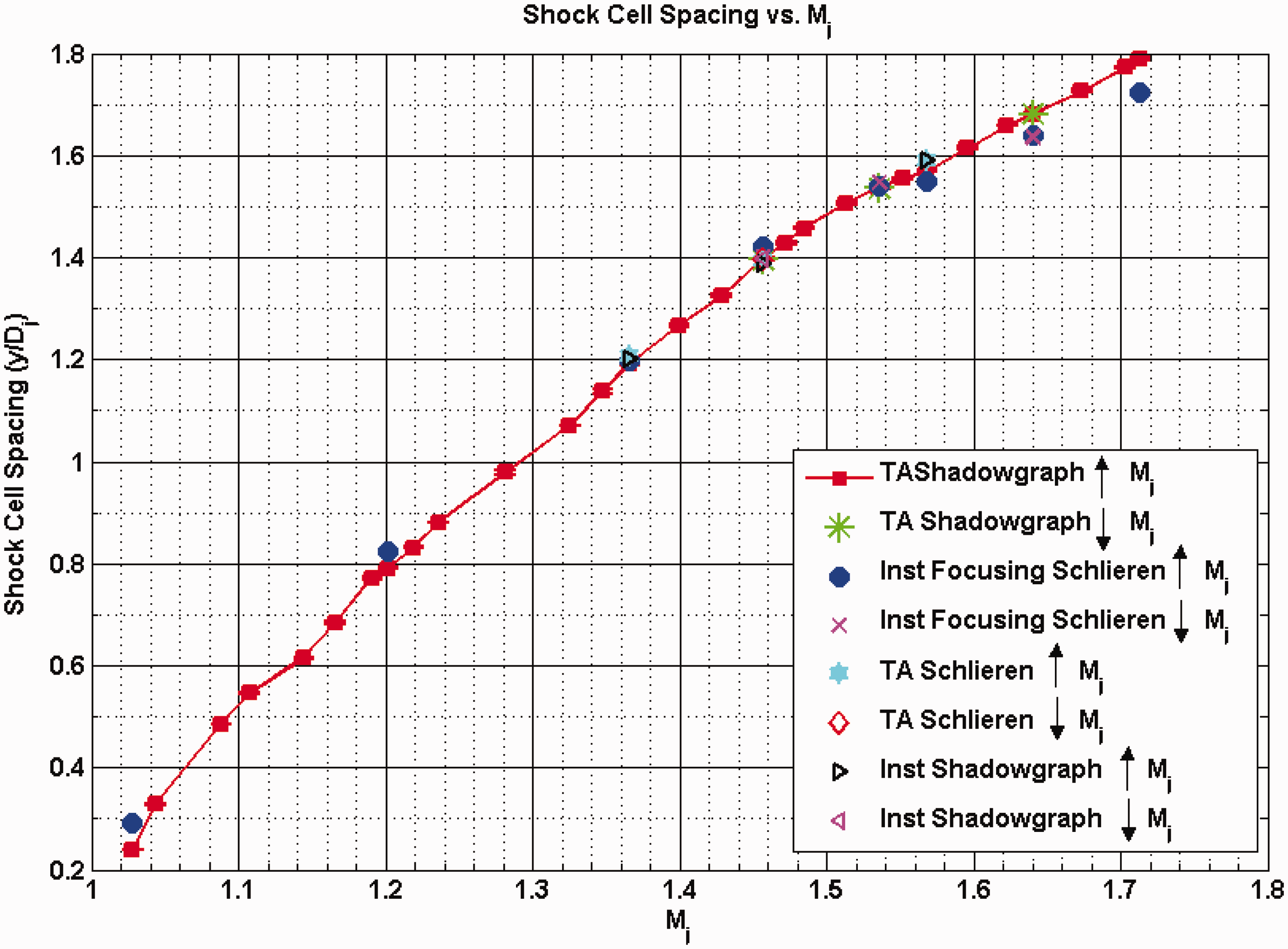

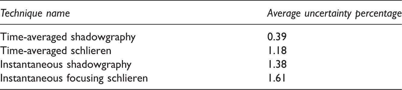
The shock-spacing data clearly displays a monotonic trend (a similar trend was noted in Clem et al.²² using the BOS technique albeit with larger uncertainty due to poorer spatial resolution). As M_j increases, the shock-spacing increases as well. The uncertainty in percentage of the average mean value for each technique (discussed in “Results and discussion”) is shown in Table 1. As stated before, it can be seen that time-averaged shadowgraphy resulted in the lowest uncertainty; whereas instantaneous focusing schlieren had the highest uncertainty due to high levels of background noise and flow turbulence obscuring the shock cell locations.

Table 1.

Uncertainty of shock-spacing in percentage of average mean value for each flow visualization technique.

Technique name	Average uncertainty percentage
Time-averaged shadowgraphy	0.39
Time-averaged schlieren	1.18
Instantaneous shadowgraphy	1.38
Instantaneous focusing schlieren	1.61

All data, within the uncertainty, do not show any abrupt changes from the monotonic behavior in Figure 7. In particular, the pairs of data in the stage jumps within the hysteresis loops are practically identical. These results leave little doubt that the shock-spacing do not go through an abrupt change during the stage jumps. Note for example that, at M_j = 1.46 (Figure 5(a)), the frequency jump is more than 20%. If a change in shock-spacing were to explain the change in wavelength causing the frequency jump, a 20% change in shock-spacing would be expected. This is clearly not the case. Therefore, it is concluded that an abrupt change in shock-spacing is neither the trigger for or associated with a stage-jump. Other parameters within the feedback loop, such as, convection velocities or changes in the growth and decay of the instability waves of different mode shapes, might be responsible for the stage-jumps. To the best of the authors’ knowledge, very few past works ventured hypotheses regarding the cause of stage-jumps. A possibility proposed in connection with the numerical experiments of Shen and Tam¹⁷ is worth mentioning. It was proposed that there might be two ways for the acoustic feedback: one by coherent scattering from the shock cells and the other via an “upstream propagating acoustic mode of the jet flow”. The authors reasoned that the former is responsible for the A₁ and B modes while the latter for the A₂ and the C modes seen in their simulation. However, it is apparent that these ideas remain to be substantiated. Further research is needed and this is considered beyond the scope of the present effort.

Conclusions

Various flow visualization techniques were employed to study shock-spacing in a 37.6 mm round, convergent nozzle over the jet Mach number range 1.0 < M_j < 1.7. These data were analyzed vis-à-vis screech frequency data to examine if abrupt changes in shock-spacing took place during stage-jumps. Time-averaged shadowgraphy, which resulted in the most clear and crisp shock boundaries, was used to determine the shock-spacings with the least amount of uncertainty. A dataset was created, from shadowgraphy as well as other techniques, to study the shock-spacing behavior associated with the screech phenomenon especially during hysteresis of stage-jumps. The data as a function of M_j follow a monotonic trend without any discontinuities across the stage jumps. Thus it is concluded that the stage-jumps are not triggered by an adjustment of shock-spacing. Shock-spacing is a continuous function of M_j. It is speculated that other parameters, such as convection velocities in different segments of the feedback loop or changes in the growth and decay of the instability waves must be at the root of the stage-jump behavior.

Footnotes

Declaration of conflicting interests

The author(s) declared no potential conflicts of interest with respect to the research, authorship, and/or publication of this article.

Funding

The author(s) disclosed receipt of the following financial support for the research, authorship, and/or publication of this article: Support from the Commercial Supersonic Technology (CST) and Transformational Tools and Technologies (TTT) Projects of NASA’s Advanced Air Vehicles Program and Transformative Aeronautics Concepts Program are gratefully acknowledged.

Appendix

References

Powell

. On the mechanism of choked jet noise. Proc Phys Soc Lond 1953; B66: 1039–1056.

Raman

. Supersonic jet screech: Half-century from Powell to the present. J Sound Vib 1999; 225: 543–571.

Tam

CKW

. Supersonic jet noise. Annu Rev Fluid Mech 1995; 27: 17–43.

Shen

Tam

CKW

. Numerical simulation of the generation of axisymmetric mode jet screech tones. AIAA J 1998; 36: 1801–1807.

Walker

Thomas

. Experiments characterizing nonlinear shear layer dynamics in a supersonic rectangular jet undergoing screech. Phys Fluids 1997; 9: 2562–2579.

Westley R and Woolley JH. The near field sound pressures of a choked jet during a screech cycle: Aircraft engine noise and sonic boom. AGARD CP No. 42, 23-1 to 23-13, 1969.

Powell

. Observations of the oscillation modes of choked circular jets. J Acoust Soc Am 1992; 92: 2823–2836.

Raman

. Advances in understanding supersonic jet screech: Review and perspective. Prog Aerosp Sci 1998; 34: 45–106.

Panda

. An experimental investigation of screech noise generation. J Fluid Mech 1999; 378: 71–96.

10.

Panda

. Shock oscillation in underexpanded screeching jets. J Fluid Mech 1998; 363: 173–198.

11.

Edgington-Mitchell D, Duke D, Amili O, et al. Measuring shear layer growth rates in aeroacoustically forced axisymmetric supersonic jets. In: Aviation 2015 conference, Dallas, TX, USA, AIAA Paper 2015-2834, 2015.

12.

Norum TD. Control of jet shock associated noise by a reflector. AIAA Paper 84-2279, 1984.

13.

Zaman

KBMQ

. Spreading characteristics of compressible jets from nozzles of various geometries. J Fluid Mech 1999; 383: 197–228.

14.

Davies

Oldfield

DES

. Tones from a choked axisymmetric jet. I. Cell structure, eddy velocity and source locations and II. The self excited loop and mode of oscillation. Acustica 1962; 12: 257–277.

15.

Gutmark

Schadow

Bicker

. Mode switching in supersonic circular jets. Phys Fluids A 1989; 1: 868–873.

16.

Ponton

Seiner

. Acoustic study of B helical mode for choked axisymmetric nozzle. AIAA J 1995; 33: 413–420.

17.

Shen

Tam

CKW

. Three-dimensional numerical simulation of the jet screech phenomenon. AIAA J 2002; 40: 33–41.

18.

Pack

. A note on Prandtl’s formula for the wavelength of a supersonic gas jet. Quart J Mech Appl Math 1950; 3: 173–181.

19.

Tam

CKW

Jackson

Seiner

. A multiple-scales model of shock-cell structure of imperfectly expanded supersonic jets. J Fluid Mech 1985; 153: 123–149.

20.

Morris

Bhat

TRS

Chen

. A linear shock-cell model for jets of arbitrary exit geometry. J Sound Vib 1989; 132: 199–211.

21.

Samimy

Zaman

KBMQ

Reeder

. Effect of tabs at the nozzle lip on the flow and noise field of an axisymmetric jet. AIAA J 1993; 31: 609–619.

22.

Clem MM, Zaman KBMQ and Fagan AF. Background oriented schlieren applied to study shock spacing in a screeching circular jet. AIAA Paper 2012-403, 2012.

23.

Merzkirch

. Flow visualization, 2nd ed. Orlando: Academic Press, Inc., 1987.

24.

Settles

. Schlieren and shadowgraph techniques: Visualizing phenomena in transparent media, New York: Springer, 2001.

25.

Weinstein

. Review and update of lens and grid schlieren and motion camera schlieren. Eur Phys J Special Topics 2010; 182: 65–95.

26.

Fagan AF, L’Esperance D and Zaman KBMQ. Application of a novel projection focusing schlieren system in NASA test facilities. AIAA Paper 2014-2522, 2014.

27.

Coleman

Steele

. Experimentation and uncertainty analysis for engineers, New York: John Wiley & Sons, Inc., 1989.

28.

Dieck RH. Measurement uncertainty: Methods and applications. Instrument Society of America, USA, 1992, Unit 2.