Jet noise computation based on enhanced DES formulations accelerating the RANS-to-LES transition in free shear layers

Abstract

The paper presents jet noise computations performed using the original and some recently proposed modified formulations of detached-eddy simulation, based on alternative definitions of the subgrid length-scale and/or a modified version of the subgrid Spalart-Allmaras model, which involves the Wall-Adapting Local Eddy-viscosity model. The modifications are aimed at the elimination or, at least, a significant weakening of a known flaw of detached-eddy simulation, namely, the severe delay of the Kelvin–Helmholtz instability and transition from fully modeled to mostly resolved turbulence in the free and separated shear layers. This flaw makes the original detached-eddy simulation formulation, in fact, non-applicable to the prediction of the noise of high Reynolds number jet flows when typical grids are used, and has led to the use of Implicit Large-Eddy Simulation instead. Based on examples of application of these modifications to such flows, already available in the literature, they were found capable of resolving the issue and providing quite accurate predictions of the aerodynamic characteristics and turbulent statistics of the high-Re jets. The study performed in the present work allows us to draw a similar conclusion regarding the accuracy of the enhanced detached-eddy simulation formulations in terms of jet-noise prediction. The new formulation gives noise results very close to those of ILES except at the highest frequencies, while being more general and less sensitive to grid resolution. In addition, it removes a (1–3) dB underestimation of the noise spectral maximums for the peak radiation direction, which is typical of ILES on fine grids.

Keywords

Jet noise computation Detached eddy simulation Free shear layers Delay of RANS-to-LES transition

Introduction

Since its conception in 1997,¹ the detached-eddy simulation (DES) method, with its later extensions and improvements (delayed DES (DDES)² and improved DDES (IDDES)³) aimed at increasing the reliability and widening the applicability of the original formulation, has become a powerful computational tool for complex aerodynamic and aeroacoustic problems. However, some DES-related issues still remain unresolved. This, first of all, concerns the so-called “Grey Area” issue. In the free shear layers and jet flows, this issue manifests itself in a significant delay of the natural Kelvin–Helmholtz instability and “secondary transition” to turbulence. This delay prevents a plausible representation of turbulence in the initial regions of the shear layers, in general, and jets, in particular, which drastically deteriorates the jet-noise prediction⁴ the present study is devoted to. The general reasons of the delay are discussed in detail by Shur et al.⁵ Its origin is associated with peculiarities of the grids typically used in DES of jet flows. In particular, in order to capture the initial jet region, these grids are refined across the jet shear layers and, typically to a lesser extent, in the streamwise direction, but are relatively coarse in the azimuthal direction. This creates strongly anisotropic grid cells which are very different from the nearly isotropic cells assumed when Large Eddy Simulation (LES) or the LES function within DES are applied within the cut-off in the inertial range.⁶ This flaw was anticipated already in the first DES formulation¹ and is primarily related to the measure of subgrid length scale, Δ, which enters the Subgrid Scale (SGS) branch of DES and all but very few other hybrid and LES methods. Initially, in 1997¹ this measure was defined as the maximum of the cell sizes in all three directions, $Δ max \equiv max (Δ x, Δ y, Δ z)$ . This definition is actually independent of the hybrid nature of DES, and we consider it as more rational and safer definition of Δ also for an LES, in general, compared to, for example, the common definition of the subgrid length-scale as the cube root of the grid-cell volume $Δ vol = \sqrt[3]{Δ x Δ y Δ z}$ .

In the archetypal LES (and LES region in DES or similar hybrid RANS-LES methods), that is, with regular grids which have essentially cubic cells of a size Δ falling within the Kolmogorov inertial range, these definitions are nearly identical. However, when applied in unstructured and/or irregular and highly anisotropic structured grids, the definitions become far from equivalent, and even in the normal LES situation with statistically isotropic eddies near the cut-off, it is easy to see that the smaller dimensions of a strongly anisotropic grid cell do not really contribute to the grid resolution capability, and therefore should not be involved in the subgrid length-scale supplied to the SGS model. This makes the cube root definition physically unjustified. On the other hand, in the initial jet region with the azimuthal grid step much larger than the other two, the $Δ max$ definition is also sub-optimal (that is, it is too “conservative”) and leads to an excessive generation of SGS eddy viscosity. This results in effectively RANS functioning of the model, which is “safe” but defeats the Kelvin–Helmholtz (KH) instability and delays transition to resolved turbulence. Hence, if the intent is to liberate the KH instability, which is essential for jet-noise prediction, a strong decrease of the eddy viscosity compared with that provided by DES combined with $Δ max$ is needed. This is confirmed by the study of jet DES by Shurtz et al.⁷ In order to remedy the delay, they refined the grid with a multi-block strategy, until the number of points in the azimuthal direction appears to be of the order of 3000; this can be compared with the highest number we used here, namely 240. The total grid counts are not as different, because of the local refinement they used, namely 40 ċ 10⁶ for Shurtz et al., versus 23 ċ 10⁶ here. Estimating the cost ratio between the two simulations cannot be precise, because the extra cost of the multi-block strategy is code- and computer-dependent, and also because the time step is shorter in the refined grid. However, given a capable enough solver, local refinement should be viewed as a valid alternative to the formulation changes proposed here.

In the authors’ earlier studies of jet-noise,^4,8,9 this motivated disabling the eddy viscosity in the jet plume, i.e. employing implicit LES (ILES) combined with Reynolds-averaged Navier–Stokes (RANS) inside the nozzle, instead of using DES in the whole domain. The approach turned out to be rather robust and accurate for a wide range of jet flows.^10–13 However, it is zonal, which complicates its application to jets from nozzles with complex geometry,¹¹ and is not applicable to jets interacting with bodies, which is typical, for instance, of the exhaust jets of aviation engines interacting with pylons or wings and especially flaps of an airplane. So some other approaches are needed, which would be compatible with the non-zonal DES formulation, on one hand, and allow a significant decrease of the SGS viscosity in the initial jet region without deterioration of the regular SGS model activity in the rest of the flow, on the other hand.

Two types of approaches have been recently proposed along these lines.

The first approach⁵ is based on alternative, solution-dependent, definitions of the subgrid length-scale Δ in the original DES formulation, whereas the second one^14,15 relies upon the incorporation of alternative SGS models which discern between quasi-2D and developed 3D flow states. In the papers,^5,14,15 both approaches were shown to be rather efficient for the prediction of the aerodynamic characteristics of a set of both generic and fairly complex free and separated shear flows and jets without drastic grid refinement in the azimuthal direction, which justifies their further evaluation in terms of the jet-noise prediction. This is exactly the primary objective of the present study, where both approaches are applied to the computation of the far-field noise generated by a subsonic round jet. A detailed comparison of results of the simulations with experimental data is carried out, allowing an objective assessment of the capabilities of the newly proposed DES versions in terms of accuracy and efficiency.

The rest of the paper is organized as follows.

In the Formulation of the enhanced DES versions section, for the sake of completeness, formulations are presented of the abovementioned approaches. Then, in the Problem statement and numerical setup section, some aspects of the problem statement and numerics used are briefly outlined, and in the Results and discussion section results of the simulations are presented, analyzed, and compared with experiments. The Concluding remarks section gives conclusions.

Formulation of the enhanced DES versions

Below, we briefly outline the two types of modifications to the original DES formulation mentioned in the Introduction.

Modifications to the subgrid length-scale within non-zonal hybrid approaches

Sensitizing the DES cell-size measure to strongly anisotropic cells in early shear layers

The first modification of the subgrid length-scale Δ proposed and outlined in detail in Shur et al.⁵ ensures the sensitization of Δ to the strongly anisotropic cells which, as mentioned in the introduction, are typically used in DES of the quasi-2D initial jet-region. This is achieved by taking into account the direction of the local vorticity vector. For a cell with the center vector r and vertices located at $r n$ (n = 1…8), the definition reads as

\tilde{Δ} ω = \frac{1}{\sqrt{3}} max n, m = 1, 8 | (l n - l m) |

(1)

where

l n = n ω \times r n

and

n ω

is the unit vector aligned with the vorticity vector.

The quantity $\tilde{Δ} ω$ represents the diameter of the set of cross-product points, $l n$ , divided by $\sqrt{3}$ (the $\sqrt{3}$ is aimed at approximately recovering $Δ max$ for 3D turbulence computed on cubic cells) and can be visualized as the result of taking a photo of the cell from the vorticity direction, and then applying the $Δ max$ definition on the paper. Its advantage over the standard DES length-scale $Δ max$ may be easily seen, e.g. for a round jet with the axis directed along x and a grid which has in the shear layer much larger spacing in the azimuthal direction, ϕ, than in the x- and r-directions. Considering that in the initial region of the jet shear layer the vorticity vector is nearly aligned with the azimuthal direction, $\tilde{Δ} ω$ reduces to $\frac{1}{\sqrt{3}} (Δ x 2 + Δ r 2) 1 / 2$ , i.e. it is of the order $O (max {Δ x, Δ r})$ , rather than to $r Δ ϕ$ (as $Δ max$ would), which seems to be physically a plausible behavior. Hence, in the anisotropic grids used in the initial jet region, the definition (1) does not lead to a strong effect of the smallest grid-spacing (typically, $Δ r$ ) on the subgrid length-scale (as, e.g., the cube root definition would) and, at the same time, always returns Δ values smaller than $Δ max$ , i.e. it ensures a corresponding reduction of the SGS eddy-viscosity, since it directly involves Δ. In contrast to this, in fully developed 3D turbulence, $\tilde{Δ} ω$ is of the order of $max {Δ x, Δ y, r Δ ϕ}$ (i.e. it is close to the standard DES definition), except for the situations when the vorticity vector is aligned with one of coordinate-directions, in which case it reduces to $O (max {Δ x i, Δ x j})$ , i.e. again it does not involve the minimum grid-spacing.

A measure for the identification of early shear layer regions

The second modification to the standard DES subgrid length-scale definition⁵ is grid-independent and therefore, unlike the first one (equation (1)), is active on arbitrary (including isotropic) grids. It turns out to be needed because unless the grid is fine enough for accurate resolution of the vortical structures in the initial region of a thin shear layer, which is currently non-affordable, the use of the modification (1) alone does not ensure a sufficiently low (meaning close to that of ILES) level of the SGS viscosity in this region. In other words, the grid anisotropy alone is not a sufficient driver, and one needs an additional, purely kinematic, measure allowing the identification of quasi-2D flow areas, in which nearly ILES treatment is desirable for facilitating the KH instability and accelerating transition, via secondary instabilities, to resolved 3D turbulence. Such a measure, called the Vortex Tilting Measure (VTM), presents a normalized cross product of the inviscid vorticity-evolution vector $\overset{\land}{S} \cdot ω$ and the vorticity vector $ω$ itself, and reads as

VTM \equiv \frac{\sqrt{6} | (\overset{\land}{S} \cdot ω) \times ω |}{ω 2 \sqrt{3 tr (\overset{\land}{S} 2) - [tr (\overset{\land}{S})] 2}}

(2)

where

\overset{\land}{S}

is the strain tensor and

tr (\cdot)

means trace. The term

\overset{\land}{S} \cdot ω

is often called “vortex stretching term” in the literature, because it has a key effect on enstrophy, but under its effect, vorticity is re-oriented, as much as it is stretched, which made us prefer the term “vorticity evolution”.

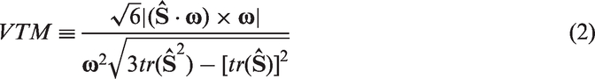
The mathematics and semantics of this formula which is an intuitive construct are explained in detail in Shur et al.⁵ and not repeated here. Note only that the VTM is bounded by 0 and 1, it is close to zero in the quasi-2D flow regions, where the vorticity vector is an eigenvector of the strain tensor (so that the cross-product in the formula is 0), and it is close to 1.0, although with very sharp downwards excursions, in developed 3D turbulence.

Combining the length-scale $Δ = \tilde{Δ} ω$ of equation (1) with the VTM quantity results in the following shear layer adapted (SLA)⁵ length-scale definition

Δ = Δ SLA = \tilde{Δ} ω F KH (< VTM >)

(3)

where the non-dimensional function

F KH (< VTM >)

is aimed at unlocking the KH instability in the initial quasi-2D region of a jet/shear layer (the angle brackets denote averaging of the

VTM

over the current and closest neighboring cells, which is needed to eliminate the abovementioned localized downward excursions experienced by the

VTM

in developed turbulence). To achieve this, the function should be small for

< VTM >

values less than some small prescribed “threshold” value, and should rapidly increase up to 1.0 as

< VTM >

increases. A specific function satisfying these demands, proposed in Shur et al.,⁵ is a simple piecewise-linear function with three segments

F KH (< VTM >) = max {F_{KH}^{min}, min {F_{KH}^{max}, F_{KH}^{min} + \frac{F_{KH}^{max} - F_{KH}^{min}}{a 2 - a 1} (< VTM > - a 1)}}

(4)

Here $F_{KH}^{max} = 1.0$ , and $F_{KH}^{min}$ , a₁, and a₂ are adjustable empirical parameters which were set equal to 0.1, 0.15, and 0.3, respectively (see Figure 1). Note that another similar function with $a 1 = 0.075, a 2 = 0.15$ and a Gaussian-shaped function also shown in Figure 1, which were tested in Shur et al.⁵ along with that defined by equation (4), have revealed only a marginal sensitivity of the results of simulations to the specific choice of the $F KH (< VTM >)$ function.

Figure 1.

Plots of different functions 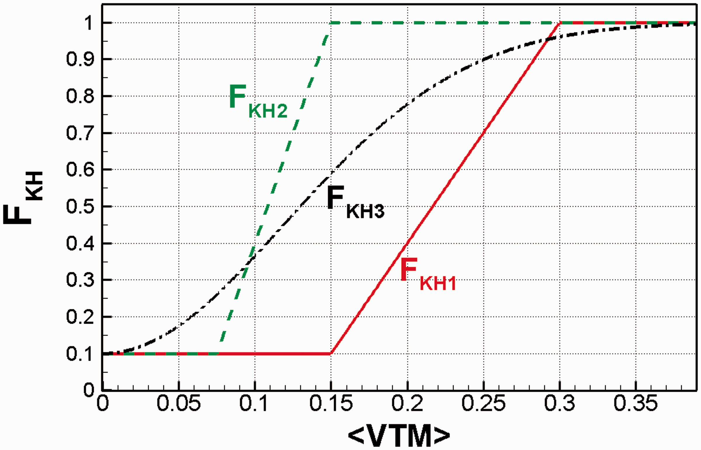$F KH$ .

Note finally that in the inviscid flow regions, the quantity < $VTM$ > strongly oscillates in space, because the vorticity vector is wavering near zero. In order to avoid possible numerical issues, this may cause near the edge of the turbulent area, the definition of the $VTM$ (2) is modified as follows

VTM = \frac{\sqrt{6} | (\overset{\land}{S} \cdot ω) \times ω |}{ω 2 \sqrt{3 tr (\overset{\land}{S} 2) - [tr (\overset{\land}{S})] 2}} max {1, \frac{ν *}{max {(ν t - ν t 0), 10 - 6 ν t 0}}}, ν * = 0.2 ν

(5)

where ν and

ν t

are the molecular and subgrid kinematic viscosities, respectively, and

ν t 0

is the freestream value of the turbulent viscosity, which was set equal to

10 - 3 ν

in the present work. This makes the

VTM

measure in the effectively inviscid flow regions sufficiently large to ensure that

F KH (< VTM >) = 1

, i.e. it is not active.

Modification of the LES branch of the SA-based DES

We in addition use the approach (SA-WALE DES), proposed in Mockett et al.¹⁴ and outlined in more detail in Fuchs et al.¹⁵ Unlike the original DES, the LES branch of which represents an SGS version of the Spalart-Allmaras (SA) RANS model¹⁶ that reduces at equilibrium (i.e. assuming that generation of turbulence is equal to its dissipation) to the algebraic Smagorinsky SGS model, the LES branch of the SA-WALE DES reduces at equilibrium to the algebraic WALE SGS model of Nicoud et al.¹⁷ An advantage of this model over the Smagorinsky one in the context of the present study is that it discerns between stable quasi-2D and developed 3D states of the flow and ensures very low levels of eddy viscosity in the former, while recovering the regular SGS model activity in the latter. Hence, in a sense, it is similar to the function $F KH$ in the subgrid length-scale defined by equation (3). Below we present a brief formulation of the LES branch of the SA-WALE DES, which is used in the jet flow simulations carried out in the present work (see the Problem statement and numerical setup and Results and discussion sections), and leave aside a somewhat more complicated full formulation of the SA-WALE DES model, which includes coupling of its LES and RANS branches (the latter can be found in the references^14,15).

The SA-WALE subgrid model is obtained from the subgrid version of the SA model by modification of the definition of the modified vorticity magnitude

\tilde{S} = S * + \frac{\tilde{ν}}{κ 2 (C DES ψ Δ) 2} f v 2, S * = (2 Ω ij Ω ij) 1 / 2

(6)

which enters the production term of the SA

\tilde{ν}

-transport equation and the definition of the parameter r of the SA model^2,16

P \tilde{ν} = C b 1 (1 - f t 2) \tilde{S} \tilde{ν}, r = \tilde{ν} / [\tilde{S} κ 2 (C DES ψ Δ) 2]

(7)

In equations (6) and (7), $Ω ij = 0.5 (\partial u i / \partial x j - \partial u j / \partial x i)$ are the components of the rotation tensor, $C b 1$ , κ and $f t 2$ , $f v 2$ are the empirical constants and functions of the SA RANS model, $C DES = 0.65$ is the constant of the SA DES, ψ is the so-called low Reynolds number correction to the SA LES (see Spalart et al.²), and Δ is the subgrid length scale.

The modification of equation (6) leading to the SA-WALE SGS model, as proposed in Mockett et al.,¹⁴ consists in replacing of $S *$ in equation (6) by the following quantity

S * \to B WALE S_{WALE}^{*},

(8)

where

B WALE

is a constant calibrated based on a simulation of decaying homogeneous turbulence^a and

S_{WALE}^{*}

is the differential operator acting on the instantaneous velocity field, which enters the expression for the subgrid eddy viscosity of the WALE LES model

(ν t) WALE = (C WALE Δ) 2 S_{WALE}^{*}

(see Nicoud and Ducros¹⁷ for the concrete expression for

S_{WALE}^{*}

In the original studies,^14,15 the capabilities of the SA-WALE subgrid model outlined above (both in isolation and in combination with the modification to the subgrid length-scale defined by equation (1)) were illustrated by examples of simulations of a free shear layer, round subsonic jet, and generic delta-wing (in the latter case, in the framework of the SA-WALE DDES). In particular, it has been shown that, as far as jets aerodynamics is concerned, if coupled with the modified length-scale (1), the approach is quite competitive with ILES.⁴ Results of its application to the jet-noise prediction are presented and discussed in the Results and discussion section.

Problem statement and numerical setup

The specific jet flow chosen for an evaluation of the different approaches to an acceleration of RANS-to-LES transition in the framework of non-zonal hybrid DES-like methods presented above is a classic round unheated subsonic jet exiting from a conical nozzle with diameter D = 0.06223 m. The Mach number of the jet at the nozzle exit is M = 0.9 and its Reynolds number based on the nozzle diameter is equal to 1.1×10⁶. The noise generated by this jet in the far-field has been studied experimentally by Viswanathan,¹⁸ and the aerodynamic characteristics of similar jets were investigated in a number of experiments.^19–23 The flow is a very common test case which has been used for validation of different numerical aeroacoustic approaches in numerous studies devoted to jet-noise prediction, including those of Shur et al.^8,9 where both the aerodynamic and noise characteristics of the jet were successfully predicted with the use of the two-stage zonal RANS–ILES approach. Hence, a primary objective of the present study is to find out if the enhanced versions of DES outlined in the Formulation of the enhanced DES versions section, which do not have the zonal ILES restrictions mentioned in the Introduction, are capable of delivering an accuracy comparable with that of ILES. Considering this, the problem statement used in the present work is similar to that employed in ILES of the jet.^4,9 For example, the flow parameters at the nozzle exit specified as the inflow boundary conditions in the LES of the jet are defined based on a precursor SA RANS computation. This emulates the practical situation of using non-zonal DDES or IDDES model for a coupled nozzle-plume computation, in which the interior of the nozzle is automatically treated by the RANS branch and the jet-plume by the LES branch of DDES/IDDES.

The other elements of the computational problem setup (computational domain, boundary conditions, and grids) and specifics of the numerics used in the present study are also similar to those used in Shur et al.^4,9 and so they are outlined here only very briefly.

All the simulations were carried out in the same computational domain⁹ which extends from 10D upstream to 70D downstream of the nozzle exit. In the radial direction, the outer radius of the domain varies from 15D in the vicinity of the nozzle to 30D at the end of the domain.

Computations were performed with the use of the compressible branch of the in-house NTS code.^24,25 It is a cell-vertex, finite-volume code accepting multi-block overset grids of Chimera type. The spatial approximation of the inviscid fluxes in the governing equations in the LES region of DES is based on the weighted (fourth order central/fifth order upwind-biased) variant of the Roe scheme²⁶ with solution-dependent weight of the upwind differences $σ upw$ ²⁷ resulting in an effectively centered scheme ( $σ upw = σ min = 0.05$ ) in the early jet shear layers. The viscous fluxes are approximated with second-order central differences. For the time integration, the implicit second-order backward Euler scheme with sub-iterations is used (a typical number of sub-iterations, ensuring at least two orders of magnitude drop of the residuals, is 10). At each sub-iteration, for the solution of the corresponding finite-difference equations, the Gauss-Seidel relaxation by planes is used, with the “sweeps” along the streamwise coordinate. The equations in each plane are solved with the line Gauss-Seidel relaxation, including trading the places of the in-plane sweep directions at the forward and backward “global” sweeps through the planes.

Finally, for the far-field noise extraction, the code employs the Lighthill acoustic analogy in the form of a modified version of the integral Ffowcs Williams and Hawkings (FWH) method²⁸ with nested closed permeable control surfaces and omitted input of the external volume integral (see Spalart and Shur²⁹ for more details). The narrowest control surface is placed in the immediate vicinity of the turbulent area in order to minimize propagation losses.

The study was designed as follows.

First, the simulations and jet-noise computation were conducted with the use of all the considered approaches on a relatively coarse grid (“Grid 2” from Shur et al.,⁹ which has about 4.2 million cells). Corresponding results are presented and discussed in the Comparative evaluation of different approaches on Grid 2 (Cases 1–6) section. After that, similar simulations were carried out on the three other grids from Shur et al.⁹ (Grid 1, Grid 3, and Grid 4 with cell count 1.6, 8.4, and 23 million, respectively – see major parameters of the grids in Table 1) with the use of only one of these approaches

Δ = Δ SLA

(3), which turned out to be most promising based on the analysis of the results of the computations carried out on Grid 2. The results of this series are presented and discussed in the Grid-sensitivity study (Cases 4, 7–9) section. Thus, the full matrix of the simulations performed includes nine cases, as presented in Table 2.

Table 1.

Key parameters of the computational grids.^a

	Grid 1	Grid 2	Grid 3	Grid 4
Outer block size $N x \times N r \times N ϕ$	308 × 81 × 64	515 × 101 × 80	515 × 101 × 160	601 × 158 × 240
Total cell count	1.6 M	4.2 M	8.4 M	23 M
$Δ x$ at nozzle exit	0.011D	0.008D	0.008D	0.005D
Average $Δ x$ for $0 < x / D < 4$	0.033D	0.022D	0.022D	0.016D
Average $Δ x$ for $4 < x / D < 10$	0.11D	0.055D	0.055D	0.042D
Min $Δ r$ in shear layer	0.003D	0.0025D	0.0025D	0.0018D
$r Δ ϕ$ in shear layer	0.05D	0.04D	0.02D	0.013D
Time step, $Δ tU 0 / D$	0.02	0.01	0.006	0.004
$St max$ ^b	2.5	7	7	12

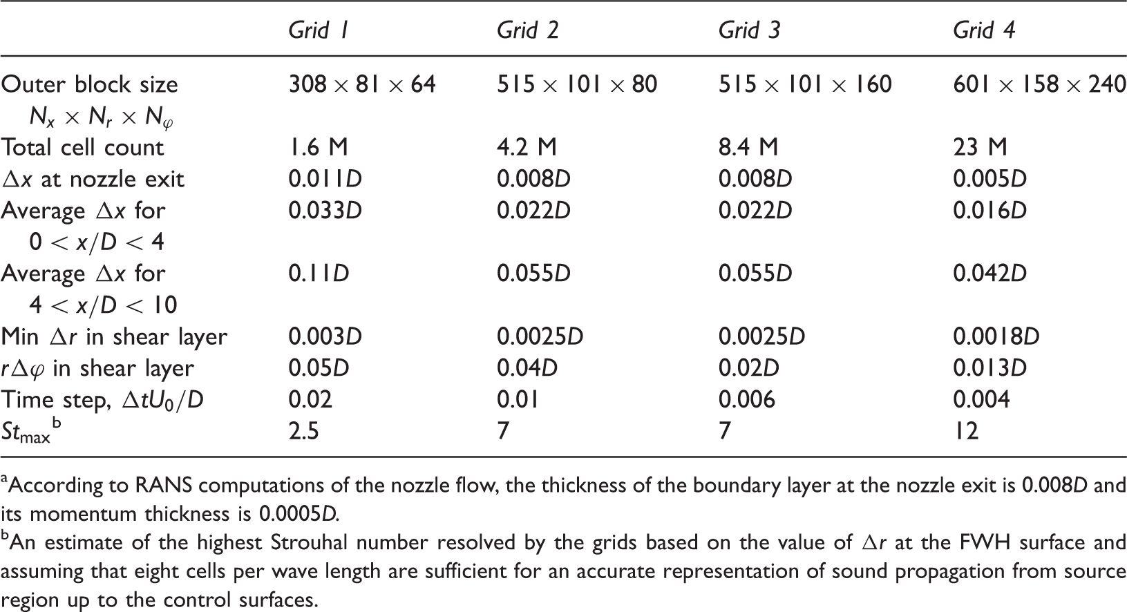
According to RANS computations of the nozzle flow, the thickness of the boundary layer at the nozzle exit is 0.008D and its momentum thickness is 0.0005D.

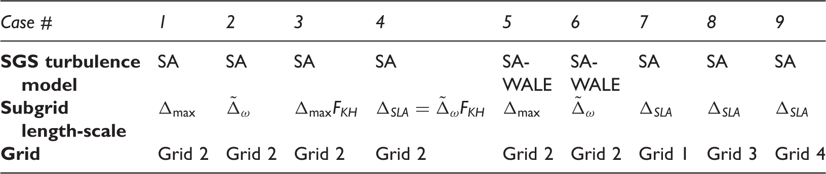
An estimate of the highest Strouhal number resolved by the grids based on the value of $Δ r$ at the FWH surface and assuming that eight cells per wave length are sufficient for an accurate representation of sound propagation from source region up to the control surfaces.

Table 2.

Matrix of simulations.

Case #	1	2	3	4	5	6	7	8	9
SGS turbulence model	SA	SA	SA	SA	SA- WALE	SA- WALE	SA	SA	SA
Subgrid length-scale	$Δ max$	$\tilde{Δ} ω$	$Δ max F KH$	$Δ SLA = \tilde{Δ} ω F KH$	$Δ max$	$\tilde{Δ} ω$	$Δ SLA$	$Δ SLA$	$Δ SLA$
Grid	Grid 2	Grid 2	Grid 2	Grid 2	Grid 2	Grid 2	Grid 1	Grid 3	Grid 4

Results and discussion

Comparative evaluation of different approaches on Grid 2 (Cases 1–6)

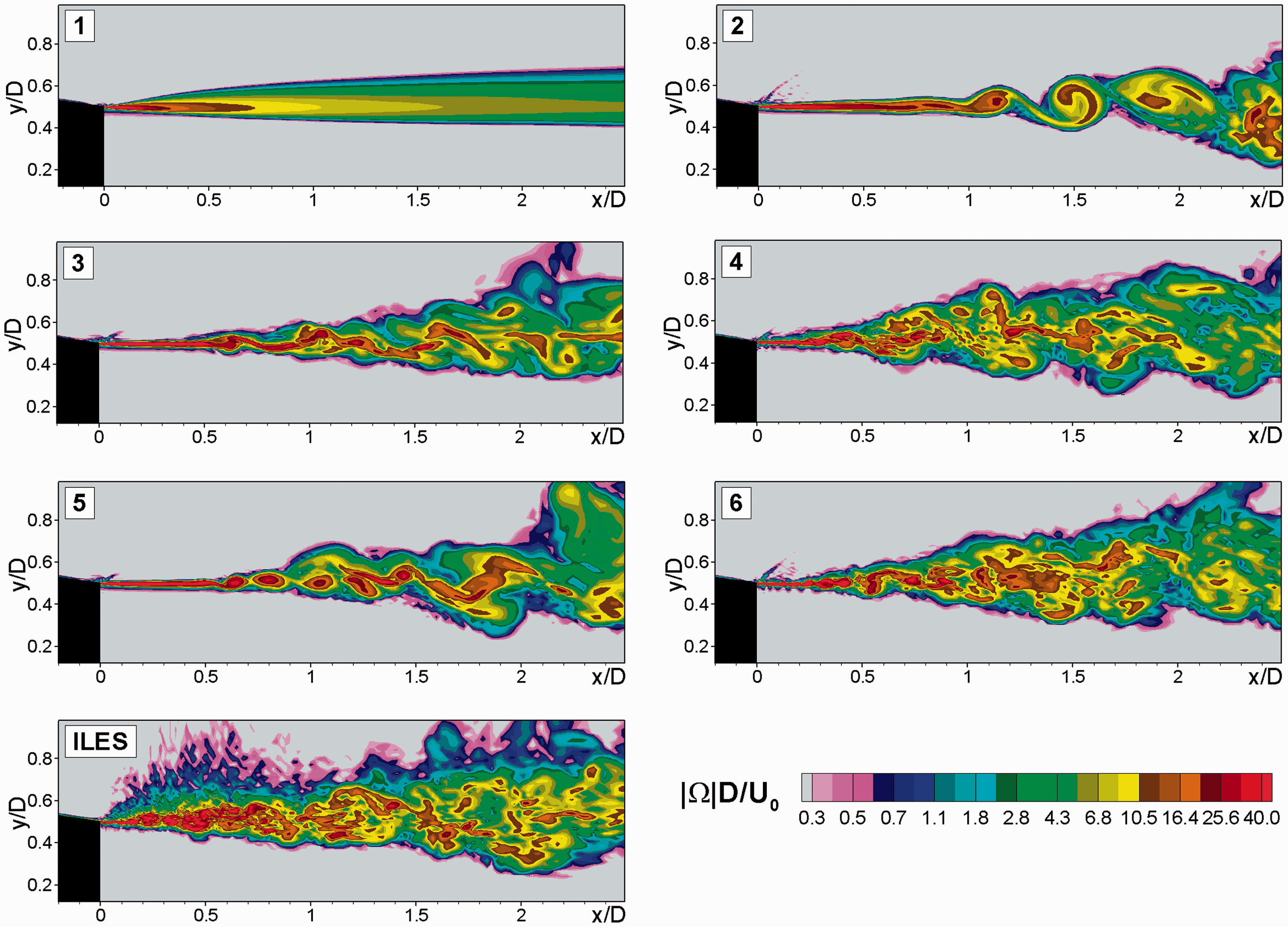
We start from the flow visualizations which visibly highlight the respective performance of the various approaches in terms of turbulence representation. In particular, the observations based on the comparison of the instantaneous fields in the meridian plane of the jet shown in Figures 2 –6 and of the radial velocity on a grid surface inside the mixing layer (Figure 7) from different simulations are as follows.

Figure 2.

Snapshots of subgrid viscosity in jet meridian plane from simulations using the SA and SA-WALE SGS models combined with different definitions of subgrid length-scale (numbers in the frames correspond to numbering of cases in Table 2). Note the exponential scale of the contours in this figure and in Figures 3, 5, and 6.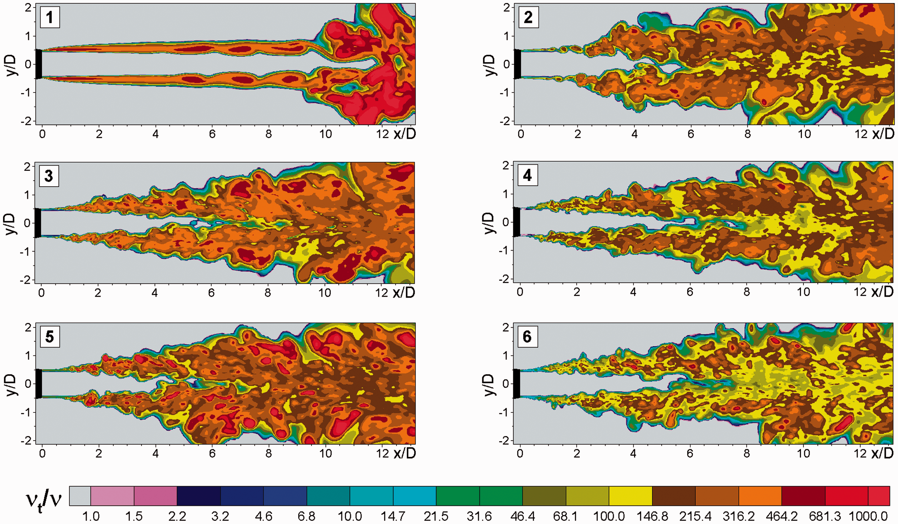

As far as the SA SGS model with different subgrid length-scale definitions is concerned (Cases 1–4 in Table 2), a comparison of the corresponding SGS viscosity snapshots in Figures 2 and 3 clearly reveals the strong decrease of $ν t$ in the initial part of the jet shear layer ensured by replacing $Δ max$ (Case 1) with $\tilde{Δ} ω$ (Case 2) and, also, by the activation of the $F KH$ function (Case 3), the most pronounced drop of $ν t$ being achieved when both modifications of the subgrid length-scale are applied simultaneously ( $Δ = Δ LSA$ , Case 4). This suggests that the modifications of the subgrid length scale act in line with their design.

Figure 3.

Same fields as in Figure 2; zoomed in on the initial part of the shear layer.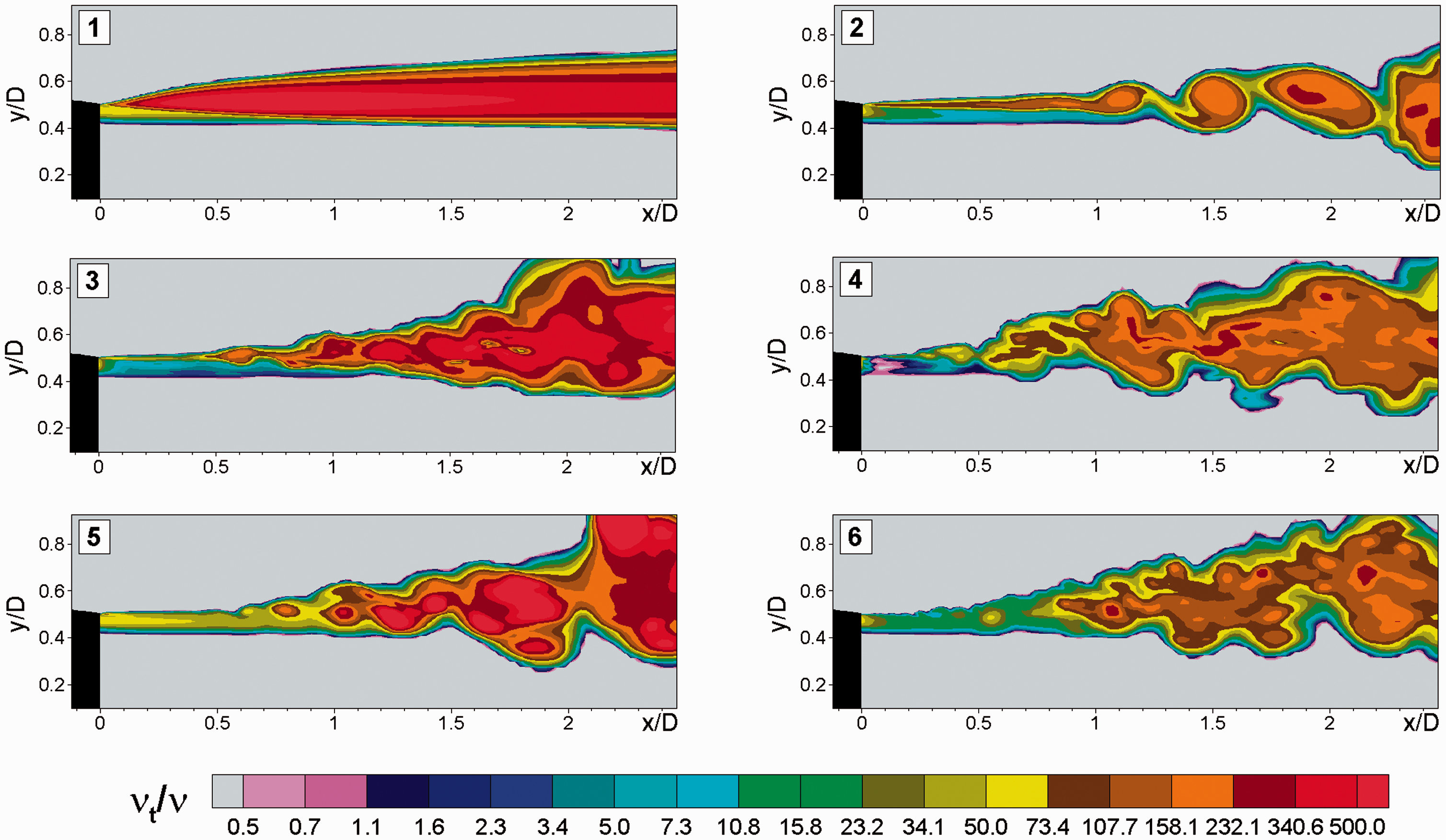

The mechanism of the action of the $F KH (< VTM >)$ function is elucidated by Figure 4 which compares snapshots of the fields of the $< VTM >$ quantity and corresponding fields of $F KH$ from simulations 3 and 4: one can see that in both cases, the function is much less than 1.0 in the early jet shear-layer and is close to 1.0 in the rest of the flow, which is exactly what causes a desirable behavior of the SGS viscosity, i.e. a strong decrease in the initial part of the jet and then remaining of the same order as that in the simulations without the $F KH$ factor in the rest of the flow. It is striking how small the region is in which $F KH$ is active, but this is of course the key region since the “mission” of this function is unlocking the KH and secondary instabilities.

Figure 4.

Snapshots of the quantity 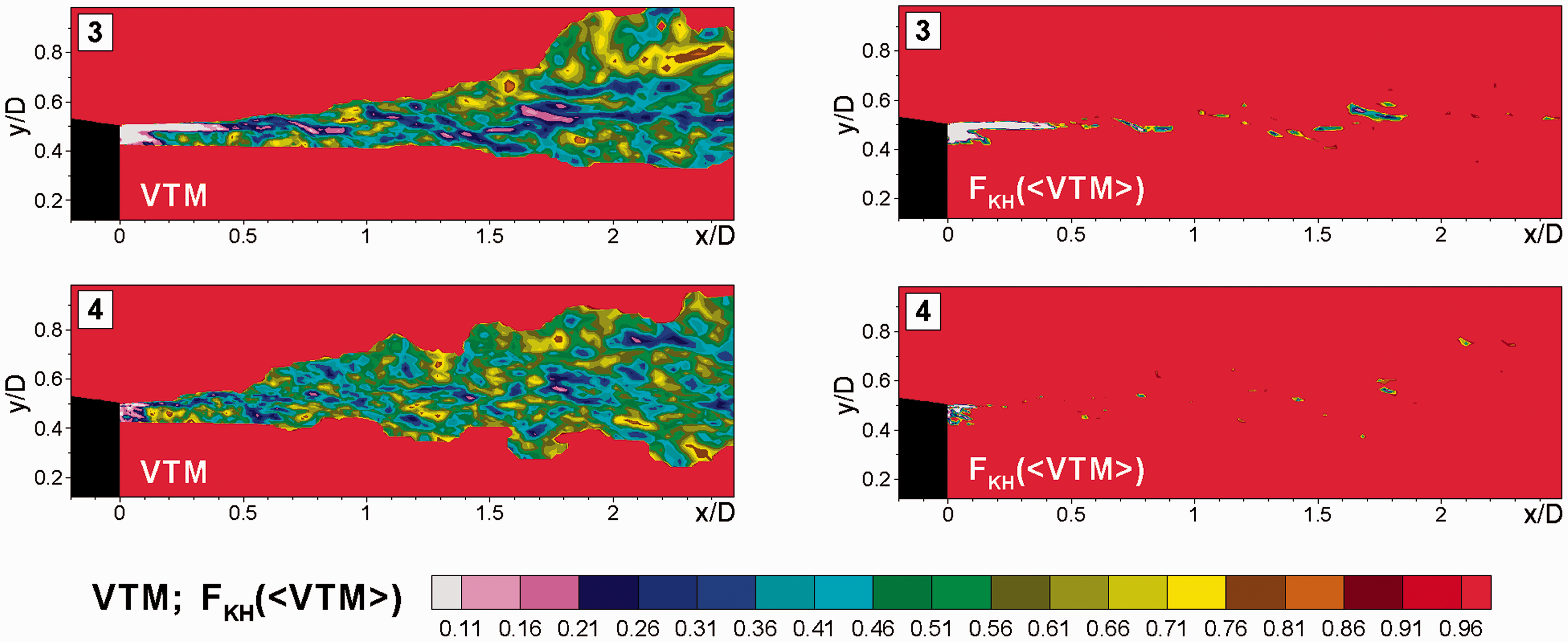< VTM > (left column) and function F_KH(<VTM>) (right column) in the jet meridian plane zoomed in on the initial part of the shear layer. Simulations using the SA SGS model combined with length-scales $Δ = Δ max F KH$ and $Δ = Δ SLA = \tilde{Δ} ω F KH$ (Cases 3 and 4 from Table 2).

As a result, as seen in Figures 5 –7, where snapshots of the vorticity magnitude and of the radial velocity inside the shear layer from the different simulations are compared, the transition from RANS to LES in the simulations with $Δ = \tilde{Δ} ω$ or $Δ = Δ max F KH$ (Cases 2 and 3) and especially in the simulation where both $\tilde{Δ} ω$ and $F KH$ factors are active, ( $Δ = Δ SLA$ , Case 4) occurs much more rapidly than in the simulation with the standard DES definition of the length-scale. Note also that exactly the simulation with $Δ = Δ SLA$ provides the turbulence representation closest to that of the ILES which is also shown in the figures. In fact, the ILES appears to contain spurious vorticity on the outside of the shear layer. Note that the exponential spacing of contours can over-emphasize this phenomenon a little. Still, the enhanced DES flow fields are visually more convincing. DES is also somewhat less sensitive to numerical dissipation than ILES.

Figure 5.

Snapshots of vorticity magnitude in a meridian plane of the jet from simulations using SA and SA-WALE SGS models combined with different definitions of subgrid length-scale (Cases 1–6 from Table 2) and from ILES.⁹

Figure 6.

Same fields as in Figure 5; zoomed in on initial part of the shear layer.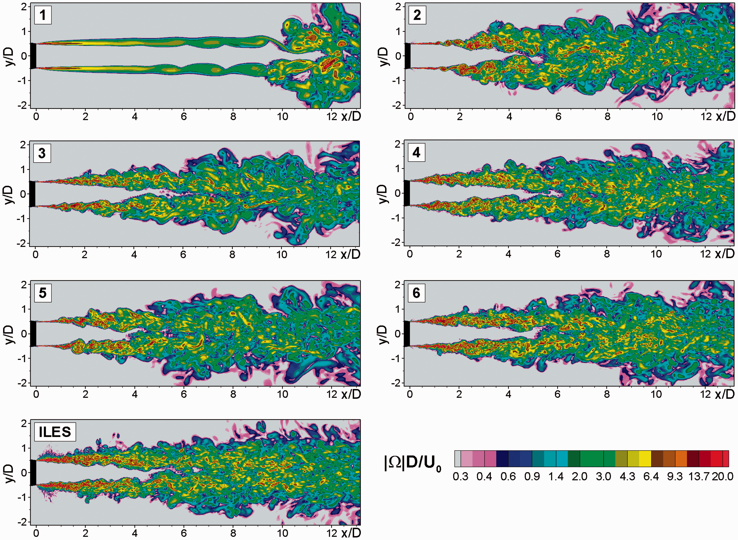

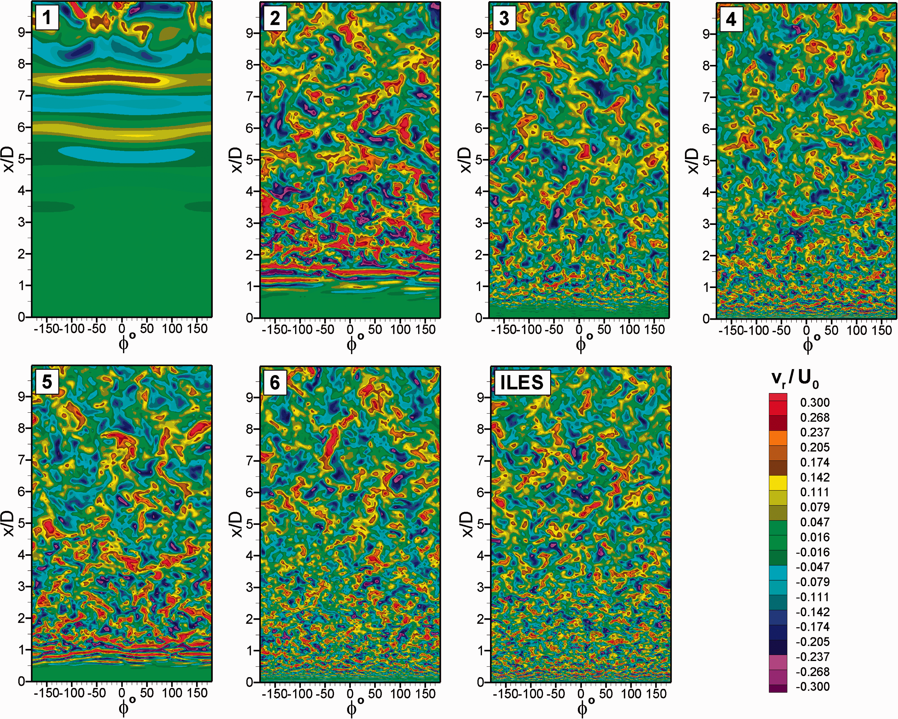
Figure 7.

Snapshots of radial velocity on a grid surface inside the mixing layer from simulations using SA and SA-WALE SGS models combined with different definitions of the subgrid length-scale (Cases 1–6 from Table 2) and from ILES.⁹

Moving to the visualizations of the SA-WALE solutions (Cases 5 and 6 from Table 2, see Figures 2, 3, 5 and 6), one can see that the model returns turbulent flow structures fairly close to those observed in Cases 3 and 4, although the effect of the use of the SA-WALE SGS model turns out to be somewhat weaker than that of the activation of the $F KH (< VTM >)$ within the SA SGS model, thus resulting in somewhat larger difference of the corresponding vorticity fields with that from the ILES.

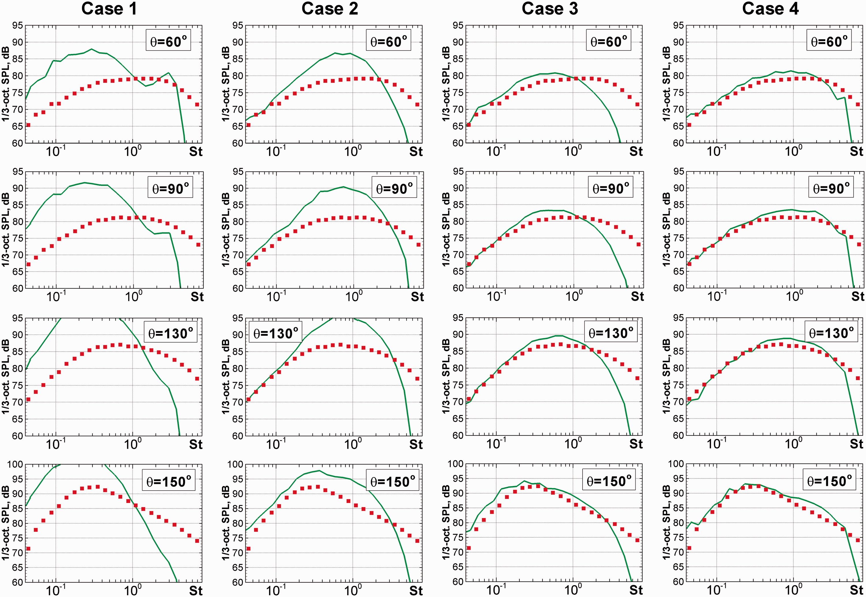
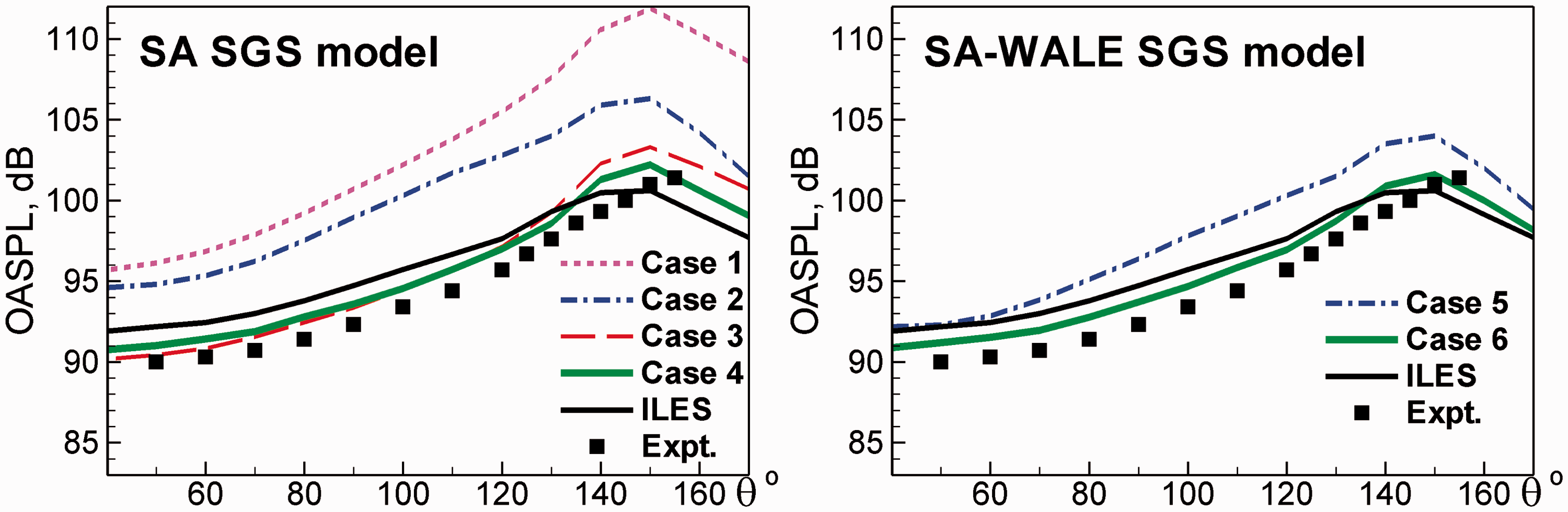
The above observations suggest that the noise computed based on the simulations relying upon the SA SGS model combined with $Δ = Δ SLA$ and with the SA-WALE SGS model combined with $Δ = \tilde{Δ} ω$ should be closest to the noise predicted by ILES and measured in the experiment. This expectation is firmly confirmed by Figures 8 and 9, where the computed 1/3-octave far-field noise spectra at four observer angles and the overall noise directivity curves from all the simulations are compared with each other, with the corresponding ILES results,⁹ and with the data of Viswanathan.¹⁸

Figure 8.

Comparison of 1/3-octave far-field noise spectra computed based on the simulations using SA and SA-WALE SGS models with different definitions of subgrid length-scale with the spectra from ILES⁹ and experiment.¹⁸ Distance 98D. Polar angle θ = 0° for upstream and 180° for downstream directions

Figure 9.

Comparison of overall noise directivities computed based on the simulations using SA and SA-WALE SGS models with different definitions of subgrid length-scale with ILES⁹ and experiment.¹⁸

The figures show, in particular, that although the SA SGS model combined with $Δ = \tilde{Δ} ω$ (Case 2) tangibly improves the noise prediction compared to the SA SGS model with $Δ = Δ max$ (Case 1), the replacement of $Δ = Δ max$ with $Δ = \tilde{Δ} ω$ alone is not sufficient for achieving an accuracy close to that of ILES. In contrast to this, the SA SGS model combined with $Δ = Δ SLA = \tilde{Δ} ω F KH (< VTM >)$ (Case 4) turns out to be quite competitive with ILES in terms of the accuracy of prediction of the noise spectra, except for their high frequency end (compare the spectra for Cases 2, 4, and ILES). This is explained by the much stronger acceleration of transition to developed 3D turbulence provided by the $F KH (< VTM >)$ function discussed above.

A similar conclusion can be made regarding the SA-WALE SGS model. For example, the positive effect of using this model alone (i.e. without modification of the subgrid length scale, Case 5) is not sufficient, whereas its combination with $Δ = \tilde{Δ} ω$ (Case 6) ensures an accuracy of the noise computation similar to that of the SA SGS model combined with $Δ = Δ SLA$ (Case 4) and ILES.

Grid-sensitivity study (Cases 4, 7–9)

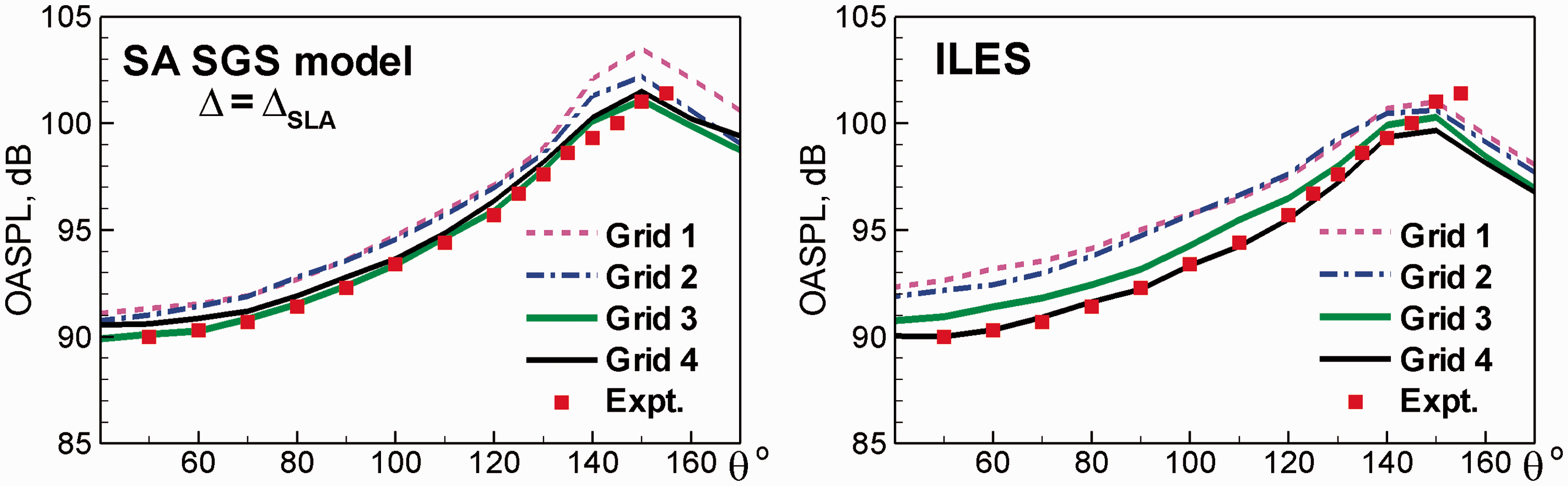
Recall that in Shur et al.,⁹ ILES of the considered jet was carried out on four successively refined grids (see Table 1). These simulations demonstrated a clear trend towards grid-convergence in terms of both the jet mean flow/turbulence statistics and the spectra/overall directivity of the noise generated by the jet. Other than that, a tangible improvement of the agreement of predicted and measured noise characteristics with grid-refinement was observed, except for the directions close to the peak radiation (θ around 150°–160°), for which the noise level was underestimated by 1–3 dB, the effect unfortunately being slightly more pronounced on finer grids.

In the present work, a similar grid-convergence study was performed in the framework of LES with the use of the SA SGS model coupled with the 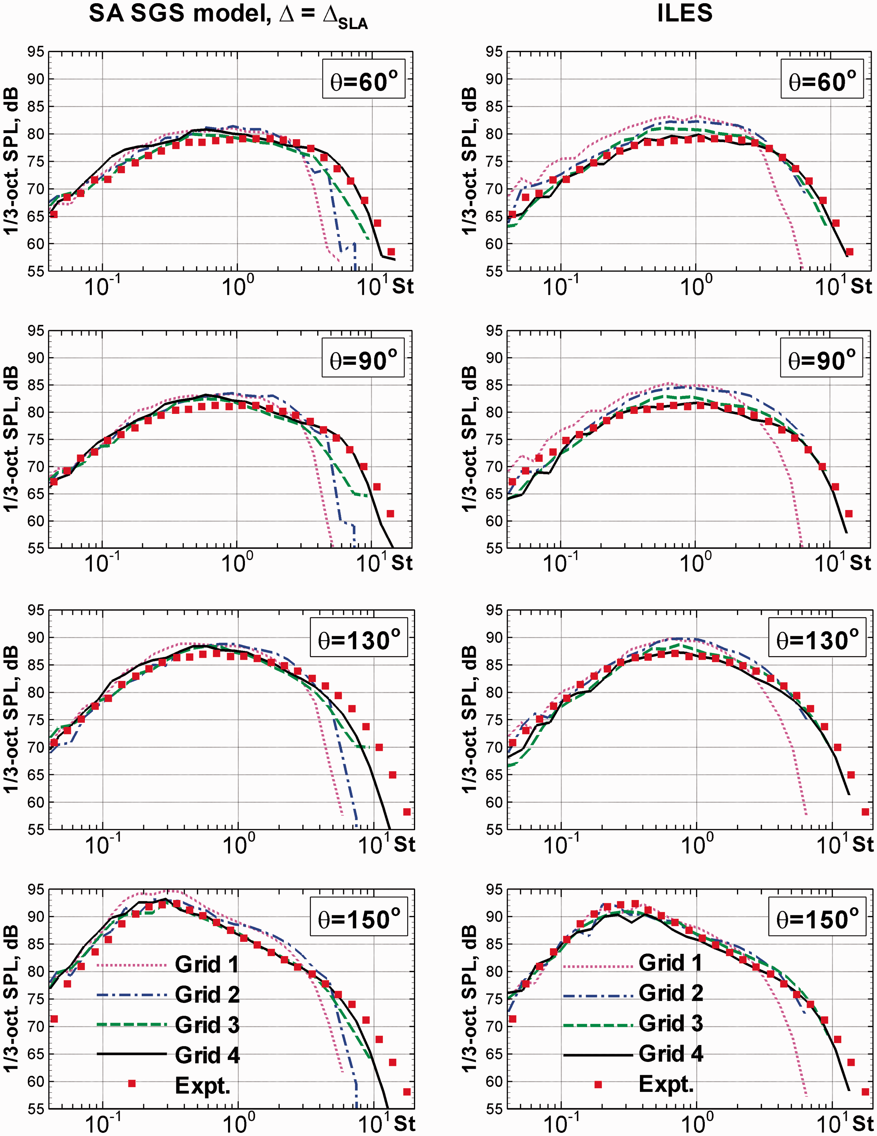$Δ = Δ SLA$ definition of the subgrid length-scale which, based on the simulations on the Grid 2 presented in the previous section, provides the most accurate noise prediction. Aeroacoustic results of this study are presented in Figures 10 and 11, together with the corresponding results from ILES.^{9
b}

Figure 10.

Effect of grid on 1/3-Octave noise spectra from simulations using SA SGS model with $Δ = Δ SLA$ (left column) and from ILES⁹ (right column). Symbols: experiment.¹⁸

Figure 11.

Effect of grid on overall noise directivity from simulations using the SA SGS model with $Δ = Δ SLA$ (left) and from ILES⁹ (right). Symbols: experiment.¹⁸

The major conclusions that can be drawn based on these figures are as follows.

First, in terms of the rate of grid-convergence of the jet noise characteristics, the explicit LES based on the SA SGS model with $Δ = Δ SLA$ actually surpasses ILES. In particular, the scatter of both the spectra (within the range of frequencies accurately represented on the corresponding grid) and OASPL curves obtained on different grids is noticeably smaller than the scatter of the ILES results, the predictions obtained on the two finest grids (Grid 3 and Grid 4) virtually coinciding with each other. This is consistent with the effect of grid on the jet mean flow parameters and turbulence statistics.⁵

Second, in contrast to the ILES noise predictions, the explicit LES does not lead to the same “noise deficit” in the vicinity of the spectral maximums for the peak radiation direction (see spectra at θ = 150° in Figure 10) and to the corresponding underestimation of the maximum of the OASPL curve (Figure 11).^c As a result, the spectra and OASPL obtained on the finest grid (Grid 4) are in a fairly good agreement with the data in a wider (virtually the whole) range of observer angles than the spectra and OASPL obtained with ILES.

On the other hand, the spectra predicted based on the SA SGS model with $Δ = Δ SLA$ reveal an earlier cut-off than the spectra from the ILES (Figure 10). For instance, for the finest grid, the estimates of the highest resolved Strouhal number are about 8.0 and 12.0, respectively. This is probably an inevitable price for using an explicit LES in which the eddy viscosity results in a stronger smoothing out of the smallest vortical structures than the numerical dissipation of the ILES. The probable spurious vorticity seen in Figure 6 for ILES does not appear to corrupt the noise prediction.

Concluding remarks

This study presents a direct continuation of the previous efforts^5,14 aimed at the elimination of the delay of transition from fully modeled to resolved turbulence in free and separated shear layers, which for many years has seemed to be an inherent flaw of DES and similar non-zonal hybrid RANS-LES approaches. A major outcome of this study is that the simple and robust proposal for its mitigation without sacrificing the non-zonal nature of DES proposed in Shur et al.⁵ turns out to be efficient not only in pure aerodynamics, but also in jet aeroacoustics. This seems to be a substantial step forward in the field of hybrid RANS-LES methodology. However, the proposed approach should still be validated for jets from complex nozzles with account of installation effects, and also for airframe noise problems where it has to be used in the framework of the fully coupled DDES/IDDES formulations.

Footnotes

Declaration of conflicting interests

The author(s) declared no potential conflicts of interest with respect to the research, authorship, and/or publication of this article.

Funding

The author(s) disclosed receipt of the following financial support for the research, authorship, and/or publication of this article: The authors from SPbPU acknowledge the financial support of the Russian Scientific Foundation (grant no. 14-11-00060).

Notes

References

Spalart PR, Jou W-H, Strelets M, et al. Comments on the feasibility of LES for wings, and on a hybrid RANS/LES approach. In: Liu C and Liu Z (eds) Advances in DNS/LES: Proceedings of the 1st AFOSR international conference on DNS/LES. Columbus: Greyden Press, 1997.

Spalart

Deck

Shur

. A new version of detached-eddy simulation, resistant to ambiguous grid densities. Theoretical Computat Fluid Dynam 2006; 20: 181–195.

Shur

Spalart

Strelets

. A hybrid RANS-LES approach with delayed-DES and wall-modelled LES capabilities. Int J Heat Fluid Flow 2008; 29: 1638–1649.

Shur

Spalart

Strelets

. Noise prediction for increasingly complex jets, Part I: Methods and tests. Int J Aeroacoust 2005; 4: 213–246.

Shur

Spalart

Strelets

. An enhanced version of DES with rapid transition from RANS to LES in separated flows. Flow, Turbulence Combust 2015; 95: 709–737.

Spalart PR. Young person’s guide to detached-eddy simulation grids, NASA CR-2001-211032. Hampton, VA: Langley Research Center, 2001, http://ntrs.nasa.gov/search.jsp?R=20010080473.

Shurtz T, Blaisdell G and Lyrintzis A. Suitability of detached eddy simulation in overflow for predicting environments near supersonic jets. In: 50th AIAA aerospace sciences meeting including the new horizons forum and aerospace exposition, Nashville, TN, 9–12 January 2012. AIAA Paper 2012-0888.

Spalart

Shur

Strelets

. Added sound sources in jets; theory and simulation. Int J Aeroacoust 2009; 8: 511–534.

Shur

Spalart

Strelets

. LES-based evaluation of a microjet noise reduction concept in static and flight conditions. J Sound Vibrat 2011; 330: 4083–4097.

10.

Viswanathan

Shur

Spalart

. Comparisons between experiment and large-eddy simulation for jet noise. AIAA J 2007; 45: 1952–1966.

11.

Shur

Spalart

Strelets

. Analysis of jet-noise-reduction-concepts by large-eddy simulation. Int J Aeroacoust 2007; 6: 243–287.

12.

Viswanathan

Shur

Spalart

. Flow and noise predictions for single and dual-stream beveled nozzles. AIAA J 2008; 46: 601–626.

13.

Shur

Spalart

Strelets

. Noise prediction for underexpanded jets in static and flight conditions. AIAA J 2011; 49: 2000–2017.

14.

Mockett C, Fuchs M, Garbaruk A, et al. Two non-zonal approaches to accelerate RANS to LES transition of free shear layers in DES. In: Girimaji S, Haase W, Peng S-H, Schwamborn D (eds) Notes on numerical fluid mechanics and multidisciplinary design, vol. 130: Papers contributed to the 5th symposium on hybrid RANS-LES methods, College Station, TX, 2015, pp.187–201. Springer.

15.

Fuchs M, Sesterhenn J, Thiele F, et al. Assessment of novel DES approach with enhanced SGS modelling for prediction of separated flow over a delta wing. In: 22nd AIAA computational fluid dynamics conference, Dallas, TX, 22–26 June 2015. AIAA Paper-2015-3433.

16.

Spalart PR and Allmaras SR. A one-equation turbulence model for aerodynamic flows. In: 30th Aerospace sciences meeting and exhibit, Reno, NV, 6–9 January 1992. AIAA Paper-1992-0439.

17.

Nicoud

Ducros

. Subgrid-scale stress modelling based on the square of the velocity gradient tensor. Flow Turbul Combust 1999; 62: 183–200.

18.

Viswanathan

. Aeroacoustics of hot jets. J Fluid Mech 2004; 516: 39–82.

19.

Lau

Morris

Fisher

. Measurements in subsonic and supersonic free jets using a laser velocimeter. J Fluid Mech 1979; 93: 1–27.

20.

Lau

. Effects of exit Mach number and temperature on mean-flow and turbulence characteristics in round jets. J Fluid Mech 1981; 105: 193–218.

21.

Simonich

Narayanan

Barber

. Aeroacoustic characterization, noise reduction and dimensional scaling effects of high subsonic jets. AIAA J 2001; 39: 2062–2069.

22.

Arakeri

Krothapalli

Siddavaram

. On the use of microjets to suppress turbulence in a Mach 0.9 axisymmetric jet. J Fluid Mech 2003; 490: 75–98.

23.

Bridges J and Wernet MP. Establishing consensus turbulence statistics for hot subsonic jets. In: 16th AIAA/CEAS aeroacoustic conference, Stockholm, Sweden, 7–9 June 2010. AIAA Paper-2010-3751.

24.

Strelets M. Detached eddy simulation of massively separated flows. In: 39th Aerospace sciences meeting and exhibit, Reno, NV, 8–11 January 2001. AIAA Paper-2001-0879.

25.

Shur M, Strelets M and Travin A. High-order implicit multi-block Navier-Stokes code: ten-years experience of application to RANS/DES/LES/DNS of turbulent flows. In: 7th Symposium on overset composite grids and solution technology, Huntington Beach, CA, 2004, http://cfd.spbstu.ru/agarbaruk/c/document_library/DLFE-42505.pdf.

26.

Roe

. Approximate Rieman solvers, parameter vectors and difference schemes. J Computat Phys 1981; 43: 357–372.

27.

Travin A, Shur M, Strelets M, et al.. Physical and numerical upgrades in the detached-eddy simulation of complex turbulent flows, Fluid Mechanics and its Applications series. In: Friedrich R, Rodi W (eds) Advances in LES of omplex flows, vol. 65, Munich, Germany: Springer, 2002, pp.239–254.

28.

Ffowcs Williams

Hawkings

. Sound generated by turbulence and surfaces in unsteady motion. Philos Transact Royal Soc 1969; A264: 321–342.

29.

Spalart

Shur

. Variants of the Ffowcs Williams–Hawkings equation and their coupling with simulations of hot jets. Int J Aeroacoust 2009; 8: 477–492.