
Abstract
The goal of this paper is to examine the computational approaches for predicting both of the overall sound pressure level (OASPL) at a few locations and acceleration power spectral density (APSD) of surrounding thin plates due to the aero-acoustic pressure generated by a cold jet with M = 1.8. First, computational fluid dynamics (CFD), particularly delayed detached eddy simulation, are applied to predict the OASPL at the near-field and compute the acoustic properties. Second, the linearized boundary element method (BEM), that is, the Helmholtz-Kirchhoff method is utilized to propagate the pressure and obtain the OASPL at the far-field. Finally, the finite element method is implemented to predict the APSD for a clamped thin plate based on the optimal triangle membrane element, discrete Kirchhoff triangle plate bending element, and Newmark-β time integration scheme. Using the present CFD and BEM, the OASPLs are compared with the experimental results measured by microphones at both the near- and far-fields, respectively. Moreover, APSDs are compared with the experimental results obtained by an accelerometer at a few different locations. Although OASPLs are overestimated because of the coarse meshes in the higher-angle area and low order scheme of the present CFD analysis, the present integrated aero-vibro-acoustic analysis is capable of predicting the OASPL and APSD generated by a cold jet with M = 1.8.
Keywords
Introduction
Vibro-acoustic phenomena are observed when either a high-speed rocket or a space vehicle is launched. The term vibro-acoustic phenomena can be classified as aerodynamic pressure fluctuation loads, self-excited loads, aero-acoustic loads, and vibro-acoustic behaviors of the launch vehicle structures. To reveal their complex nature, an integrated aero-vibro-acoustic analysis procedure is required. Bianco et al. 1 recently proposed an integrated verification approach for a Vega-C launcher by combining a semi-empirical method and a state-of-the-art hybrid finite element method (FEM)/statistical energy analysis (SEA). Although the verfication is capable of accurately predicting the vibro-acoustics in the interior of the launcher, only the verification process is presented without any validation with experimental data. The complexity of the integrated aero-vibro-acoustic analysis procedure is simply driven by the following two factors: (i) the acoustic pressure loads generated from the supersonic jet, and (ii) vibratory responses of the concerned structures induced through acoustic pressure loads.
First, the characteristics of the acoustic pressure loads generated from a supersonic jet have been reported based on the experimental results. 2 An empirical methodology has been widely used to predict the near- and far-field noise by applying normalized results obtained through acoustic measurements. A source distribution and extrapolation technique are used to develop an empirical analysis within the accuracy of ±6 [dB] for the standard configurations.2,3 Whereas Reynolds averaged Navier-Stokes (RANS) simulation is capable of achieving the potential core length of a supersonic jet, large eddy simulation (LES) techniques have received significant attention in the prediction of high-frequency propagation behavior. Haynes et al. 4 and Bodony et al.5,6 suggested that it is necessary to conduct an LES when considering the discretization scheme, boundary conditions, and far-field prediction based on the acoustic analogy, that is, the Lighthill theory. Specifically, both the Helmholtz-Kirchhoff (H-K) and Ffowcs Williams-Hawkings (FW-H) methods are employed to extrapolate sound propagation from the inner computational domain to the far-field area.7–9 A detached eddy simulation (DES) is an alternative technique to alleviate the requirement of an LES. It is extended to develop a delayed detached eddy simulation (DDES) turbulence model. 10 Based on the computational approaches mentioned above, Lo et al.11,12 conducted both fully expanded and under-expanded supersonic jet simulations at the laboratory scale using an exit Mach number of 1.95.
Second, vibro-acoustic analysis is mainly related to the structural responses owing to aero-acoustic loads generated from the supersonic jet at lift-off or static firing. To predict the structural responses from acoustic loads, the FEM was developed during the 1960s and 1970s. To couple the acoustic load and structural responses, the BEM was also adopted. Finally, the SEA approach was developed to predict the structural responses within a higher frequency range. Arenas et al. 13 explained the noise and vibration characteristics of spacecraft structures. Pirk et al. 14 conducted vibro-acoustic analysis for a Brazilian vehicle satellite launcher (VLS) fairing. To predict the dynamic response of the mechanical structure and the inner acoustic cavity of the fairing, FEM/BEM was used for a low-frequency analysis with an emphasis on the vibro-acoustic coupling effect between the fairing structural vibrations and its inner cavity acoustic pressures. However, it is still ambiguous to determine the mid-frequency range in which the structural displacement differs between the FEM/BEM and SEA analyses. Desmet 15 suggested various potential solutions to mid-frequency vibro-acoustic model, and hybrid approaches. For the design verification process of a launch vehicle (Vega-C launcher), an integrated aero-vibro-acoustic procedure was developed. 1 Supersonic jet parameters such as the diameter of the nozzle exit and the Mach number are used to assume the aero-acoustic characteristics. A semi-empirical jet noise model (revised Eldred-based model) and BEM-based propagation were adopted to predict the OASPL at the far-field. A vibro-acoustic analysis was then implemented. For the low-frequency range, both a FEM/SEA and full FEM were conducted. For the high-frequency range, an SEA analysis was adopted as well.
In this paper, a sequentially integrated aero-vibro-acoustic analysis for a cold jet and the structural responses of a clamped thin plate is proposed. Three-dimensional DDES analyses are employed to predict the acoustic noise for a small-scale supersonic jet. A procedure for applying data computed from a three-dimensional DDES to an acoustic analysis is also described while preserving the frequency range of the aero-acoustic prediction. For the far-field noise prediction, the H-K method is adopted. For the vibro-acoustic analysis, a three-dimensional transient FEM was developed based on the optimal triangle membrane element-discrete Kirchhoff triangle plate bending element (OPT-DKT)-based shell element with a Newmark-β time integration. The natural frequencies of a clamped thin plate are determined based on the frequency response function (FRF) without damping effect. By coupling the aero-acoustic loads predicted through the DDES/H-K method and a transient FEM analysis, three different APSDs for a clamped thin plate are predicted. Furthermore, an accessible equipment setup for a small-scale supersonic jet is designed and implemented. 12 and 15 sets of microphones are used to measure the sound pressure level (SPL) in both the near- and far-fields. An accelerometer is also employed to obtain APSDs for a clamped thin plate. Figure 1 describes the verification and validation process for the OASPLs and APSDs of a small-scale supersonic jet noise and a clamped thin plate. Verification and validation process of sequentially integrated aero-vibro-acoustic analysis for a small-scale supersonic jet.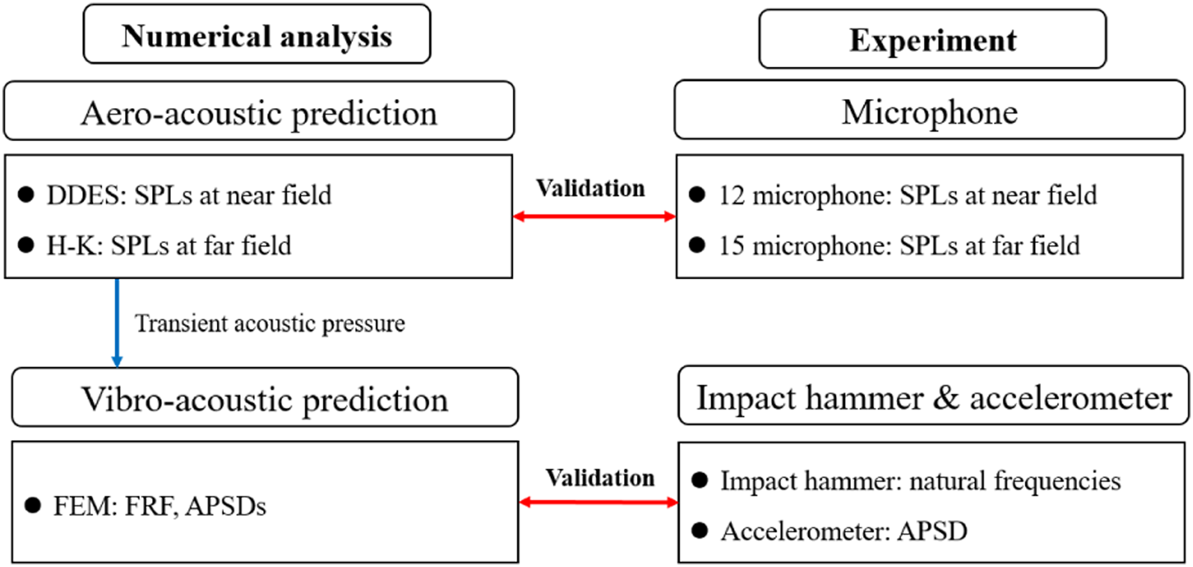
Experimental setup for a small-scale supersonic jet and a clamped thin plate
Experimental configuration for a small-scale supersonic jet
The experimental apparatus is designed to measure the SPLs of both the near- and far-field and APSDs for a clamped thin plate. First, a configuration of the small-scale supersonic jet is manufactured to have an exit Mach number 1.8. The diameter at the small-scale supersonic jet was fixed on a 20 [mm] as shown in Figure 2. Small-scale supersonic jet for exit Mach number 1.8.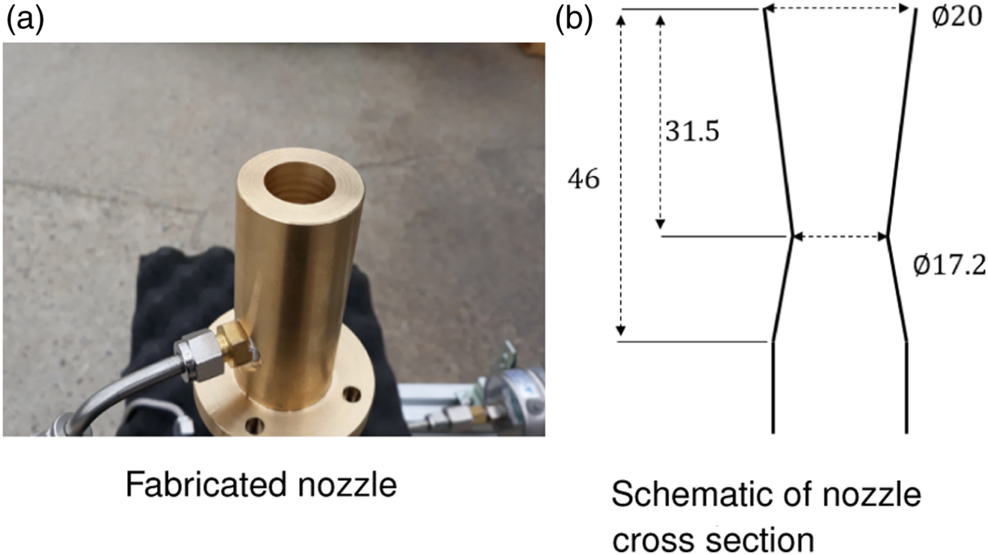
The radius at the nozzle throat was determined to be 8.6 [mm] under the assumption of an isentropic process.
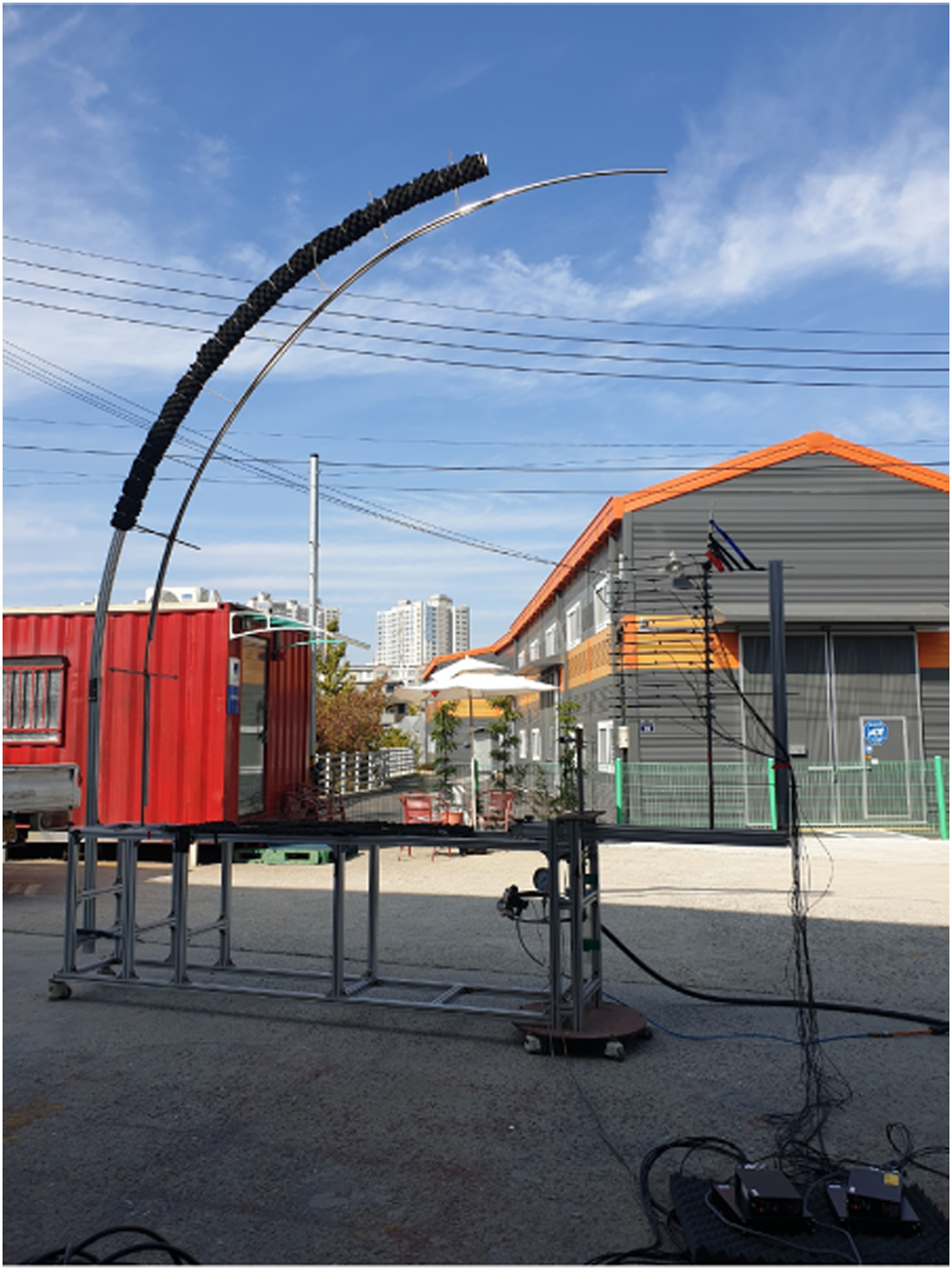
Five main components were introduced for the small-scale supersonic jet noise experiments. A number of bombe are needed to satisfy the high pressure owing to the limited capacity of approximately 12-15 [bar] each. For the present experiments, the target pressure at the inlet of the small-scale supersonic jet is 6.5 [bar], which requires at least 50 [bar] in a reservoir. An air compressor is also required to recharge the exhaust pressure for continuous experiments. A valve/regulator is equipped to adjust the required inlet conditions. Owing to the high-pressure inlet condition of the small-scale supersonic jet (6.5 [bar]), a regulator is either tightened or loosened to satisfy the high-pressure condition. A highly pressurized supersonic flow is injected upward to avoid an acoustic reflection from the bottom wall. Both the near- and far-field noises are measured using a number of microphones with a measurement band of over 160 [dB]. Two types of microphones were employed. Figures 3 and 4 describe the schematic sketch and photograph of an experimental setup for small-scale supersonic jet noise. Schematic sketch of experimental setup. Photograph of experimental setup.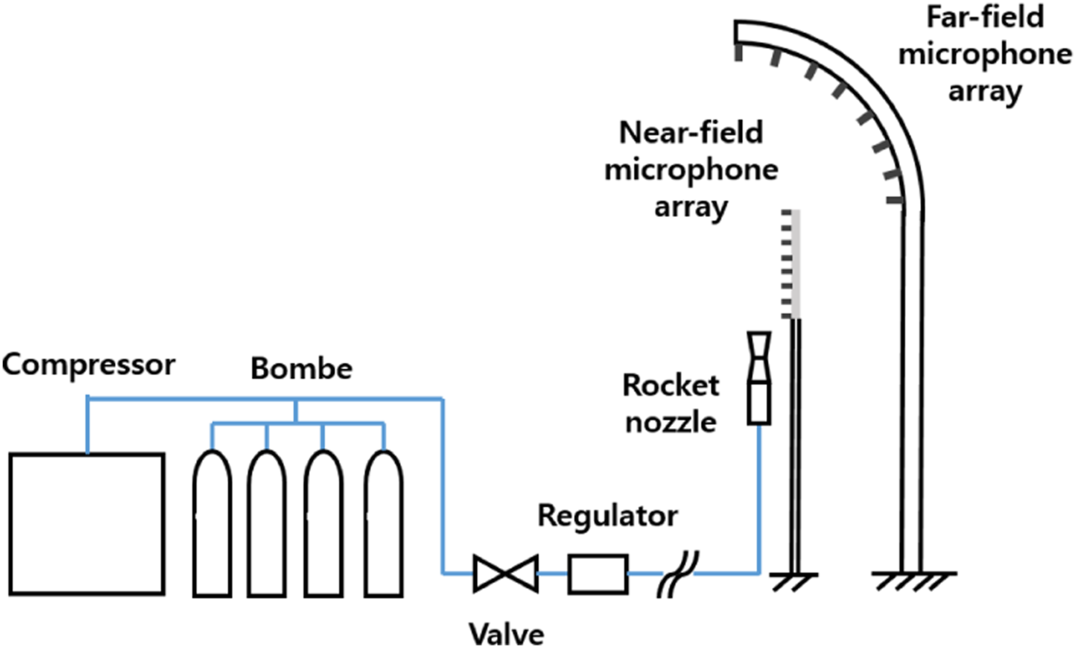
Experimental configuration for both near- and far-field array
To measure the static pressure at the near field, the microphone array should be located within the region of the dominant supersonic jet flow while avoiding fluctuations. The near-field experimental results will be used to validate the numerical results obtained through the CFD analysis. Twelve microphones are employed at a distance equal to 10-times the diameter of the nozzle. Each microphone is separated at 2.5D
e
intervals where D
e
denotes the diameter of the nozzle exit. Figure 5 describes a schematic sketch of 12 microphones equipped with additional supports. Schematic sketch of an experimental setup for the near field measurement.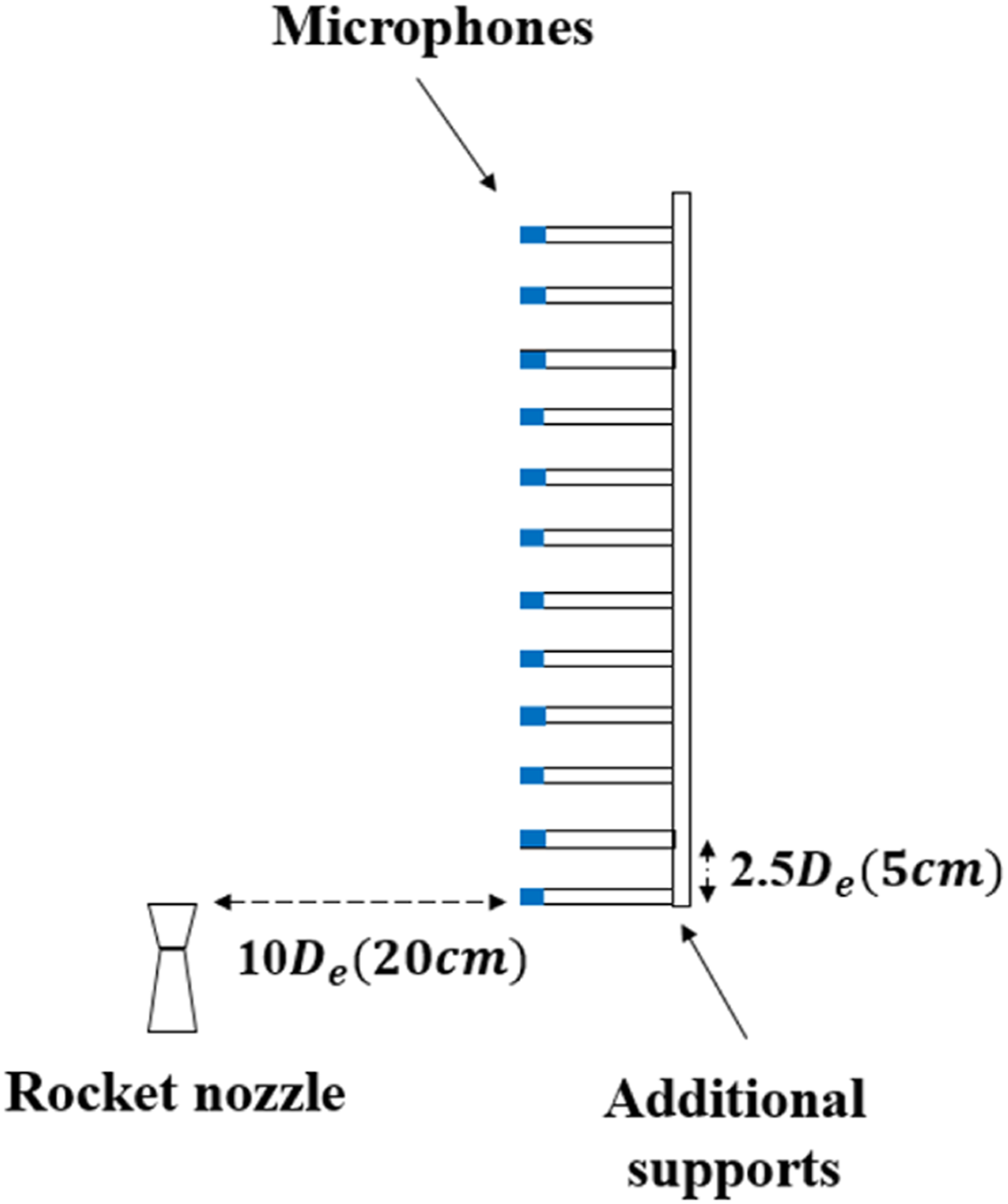
It is important to assume the noise source location for the far-field noise measurement. In accordance with the experimental results conducted by Gee et al., 16 the present noise source is assumed to be located along the axis of the jet and downstream of the jet exit plane at a distance of 13D e from the nozzle exit. An annular array of 15 microphones is equipped with the presence of noise generated from the supersonic jet flow. Each angle of 13 points varies by 5° from 20° to 80°. The remaining two points vary by 10° from 90° to 100°. The diameter of the annular array is 100D e to facilitate validation with the numerical results. Figure 6 depicts the schematic sketch of an experimental setup used for the far-field measurement. Both the additional supports and the annular array are covered with sound-absorbing materials to avoid scattering. The specifications for the two types of microphones are presented in Table 1.
Experiments were conducted more than three times to investigate the reproducibility of the small-scale supersonic jet. During the blowing of each supersonic jet, which lasts 3 [s], pressure data are measured using 12 and 15 sets of microphones in the near and far-fields, respectively. Figures 7(a) and (b) show the transient pressure history at both the near- and far-field arrays. Schematic sketch of experimental setup. Specifications for two types of microphone. Transient pressure history.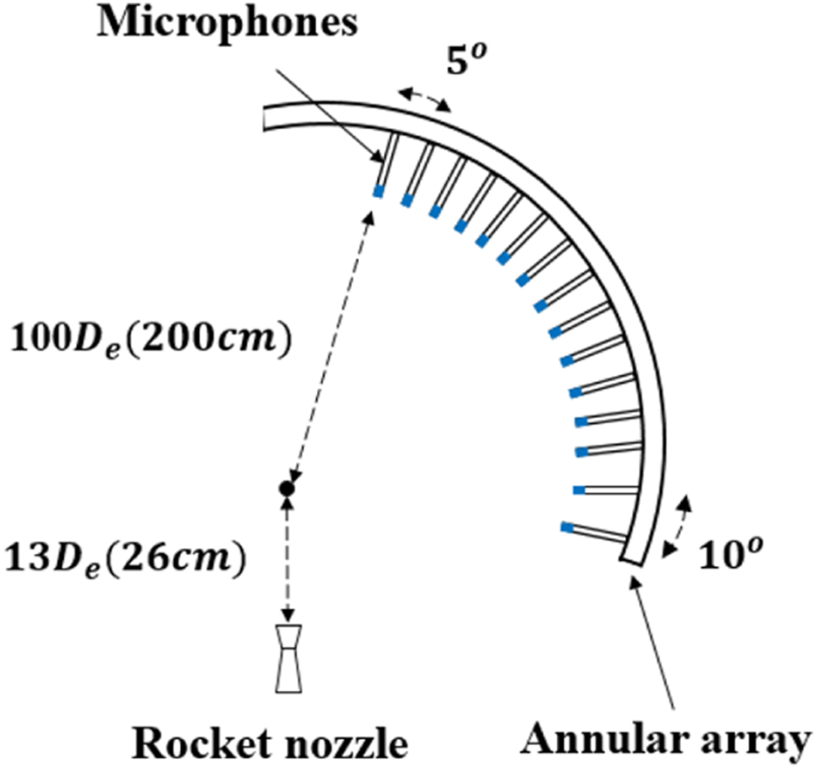
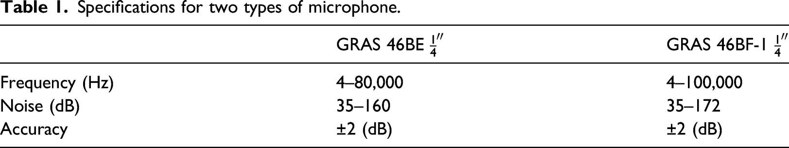
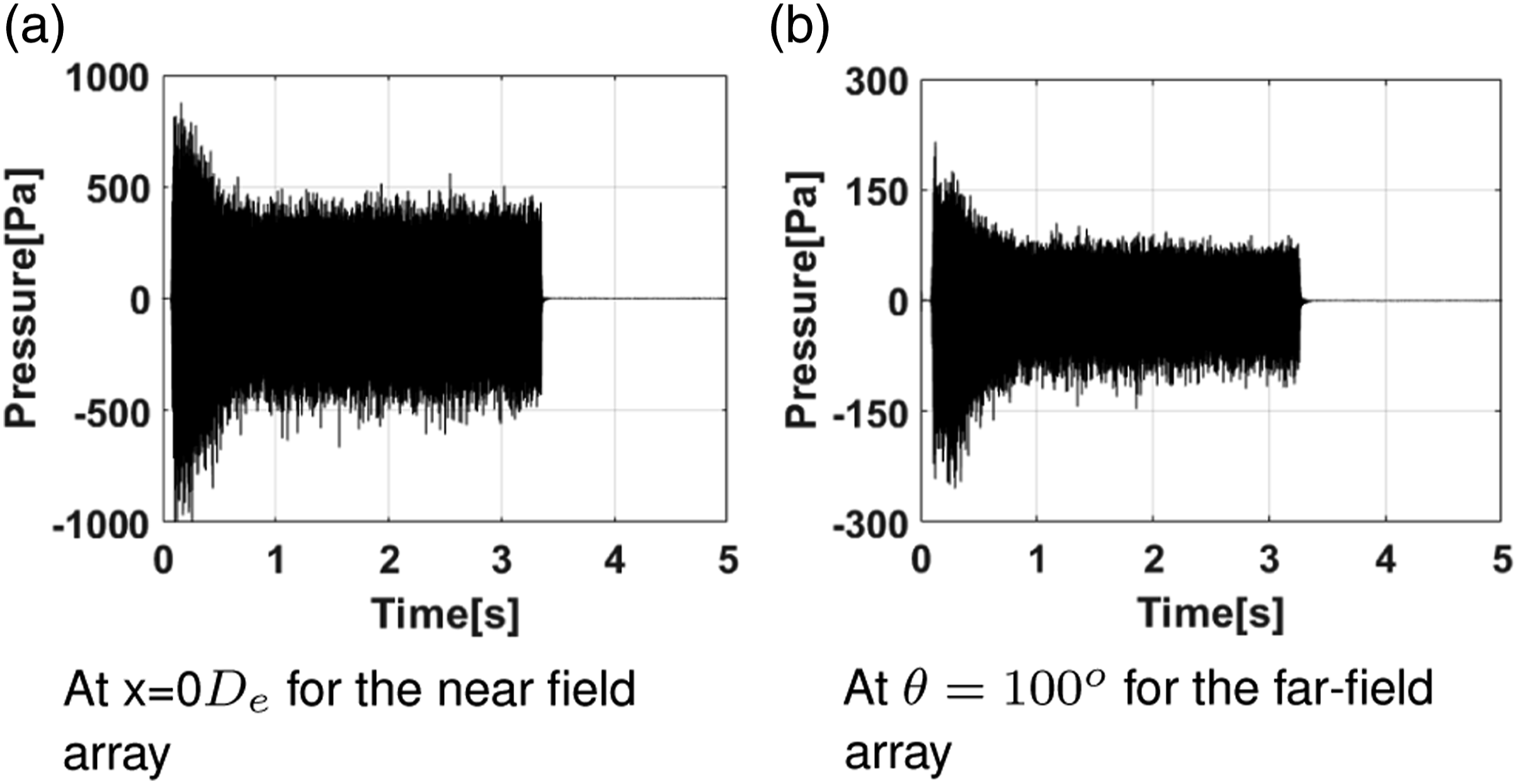
By adopting an analysis block size of 100 samples and a 50% overlap, this results in approximately 200 average value for each location. Although two microphones are capable of measuring the frequency range at up to 80 [kHz] and 100 [kHz], respectively, a fifth-order Butterworth filter with a range of 500–9600 [Hz] is employed to obtain OASPLs and power spectral densities (PSDs). Only pressure data from 1.5–2.5 [s] are employed, where the transient pressure is converged. Figures 8(a) and (b) describe the PSDs of the near and far-fields, respectively. Although the experiments are conducted in an urban area, the effect by the background noise may not be significant. The background noise located at 100–200 [Hz] and will automatically be filtered out by using the filter with a range of 500–9,600 [Hz]. From the experimental results shown in Figures 8(a) and (b), the reproducibility of the supersonic jet noise is sufficiently verified. Discrepancy no larger than 0.8 [dB] is observed at all the microphone locations. PSDs for the near-and far-field.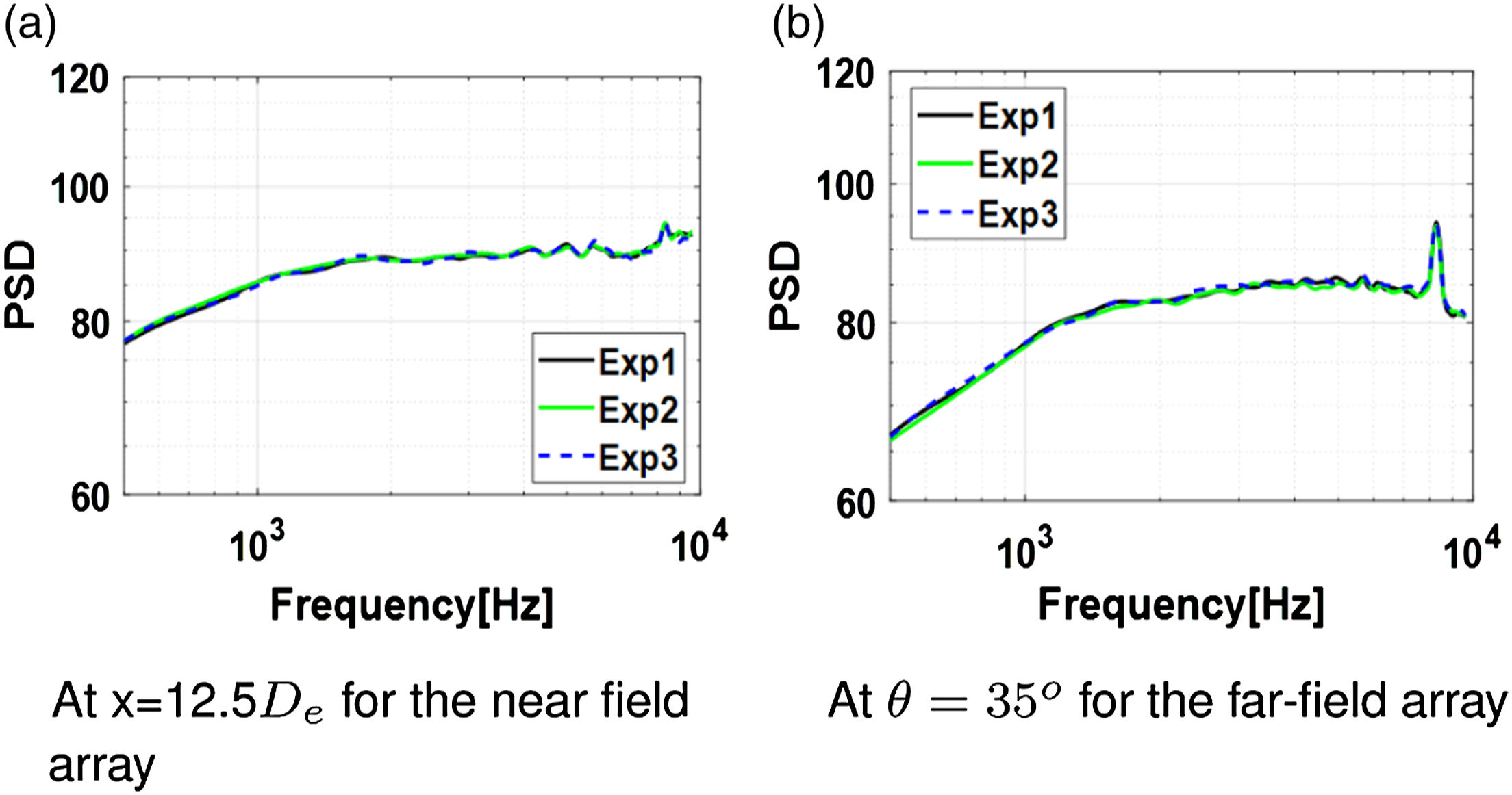
Experimental configuration for a clamped thin plate with an accelerometer
To measure the structural responses vibrated by the aero-acoustic pressure generated from a small-scale supersonic jet, a clamped thin plate at three different locations are measured. Three locations are selected to investigate the effects of aero-acoustic loads on vibrating a thin plate. Whereas Positions 1 and 3 are located at high angles from the supersonic jet, Position 2 is intentionally placed at the location where directional aero-acoustic loads are dominant. Figure 9 describes the schematic sketch of the experimental setup. Schematic sketch of an experimental setup for an oscillatory structure.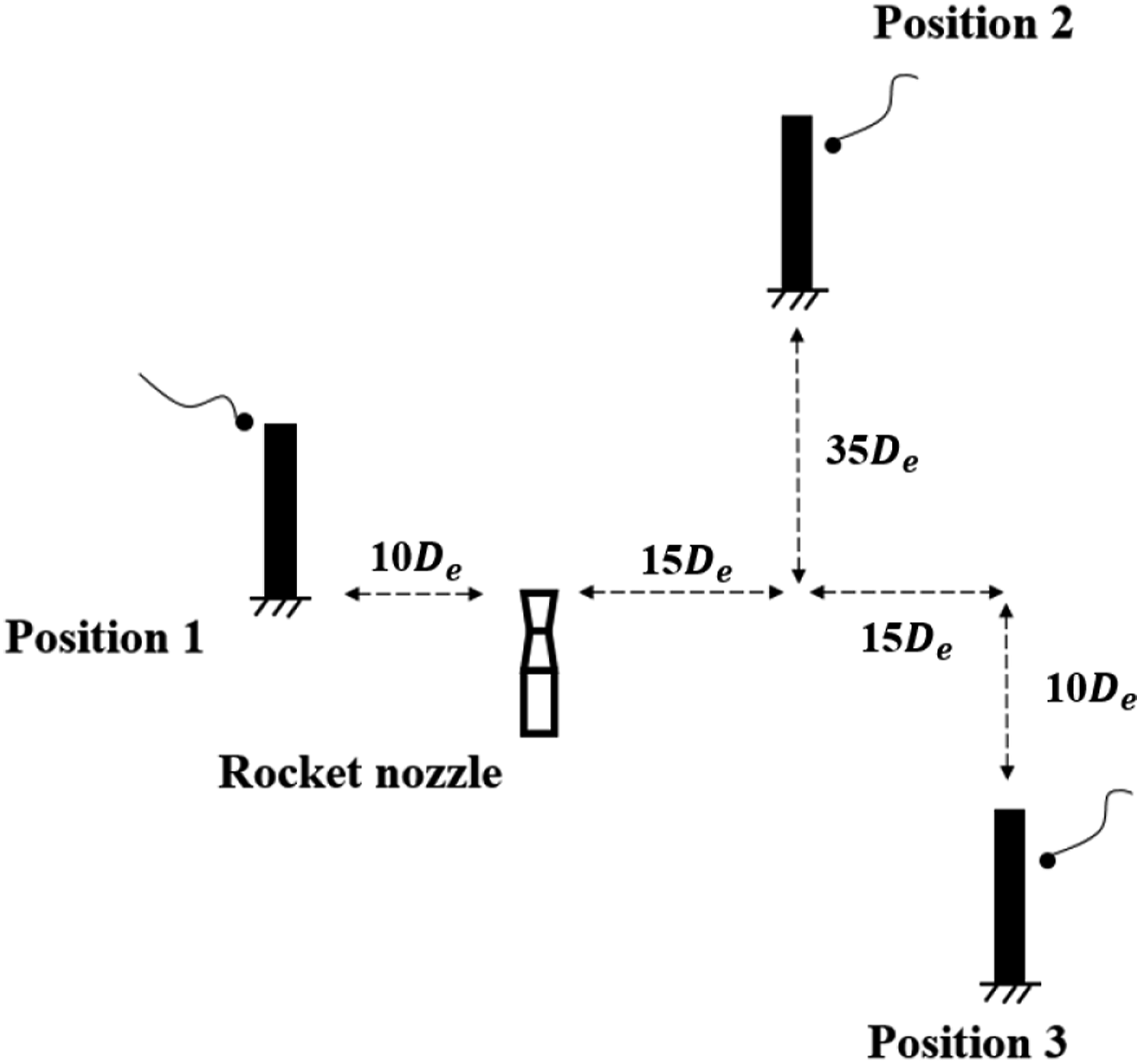
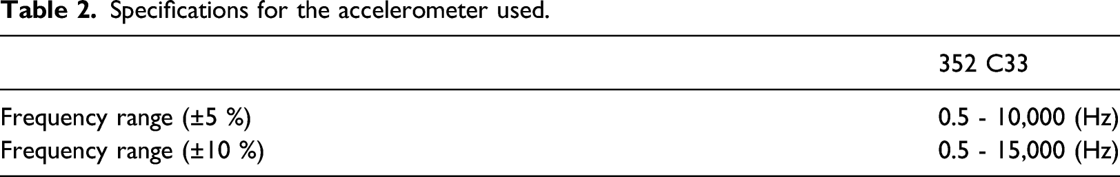
Specifications for the accelerometer used.
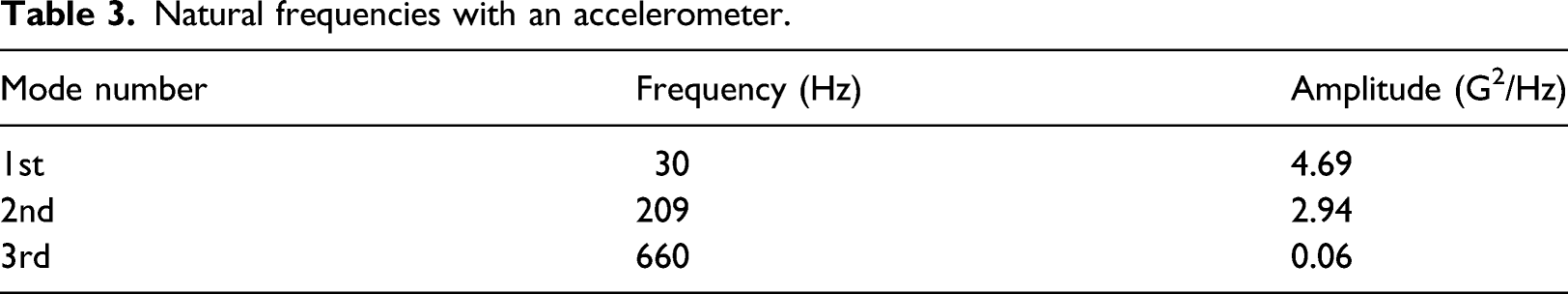
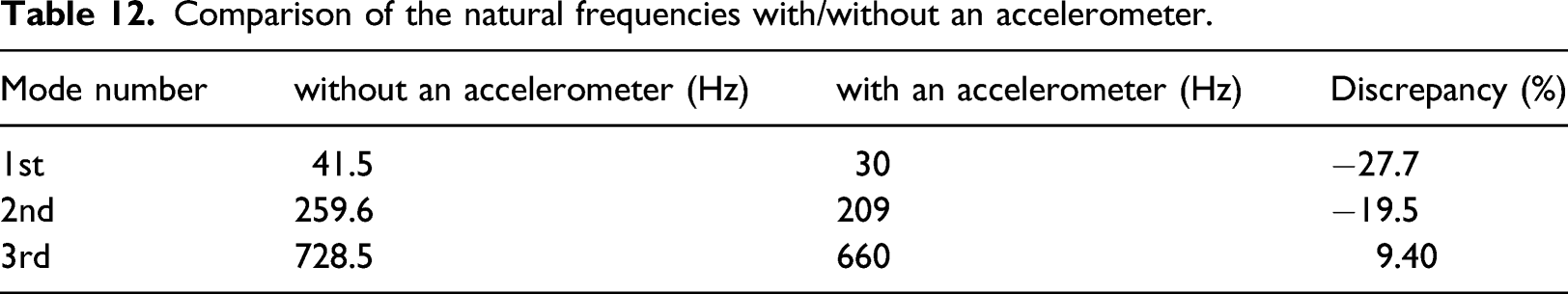
The natural frequencies of the clamped thin plate varied owing to the mass of the accelerometer used. Figure 10 and Table 3 depict the fast Fourier transform (FFT) results of the present impact hammer experiment. Fast Fourier transform results of the present impact hammer experiment. Natural frequencies with an accelerometer.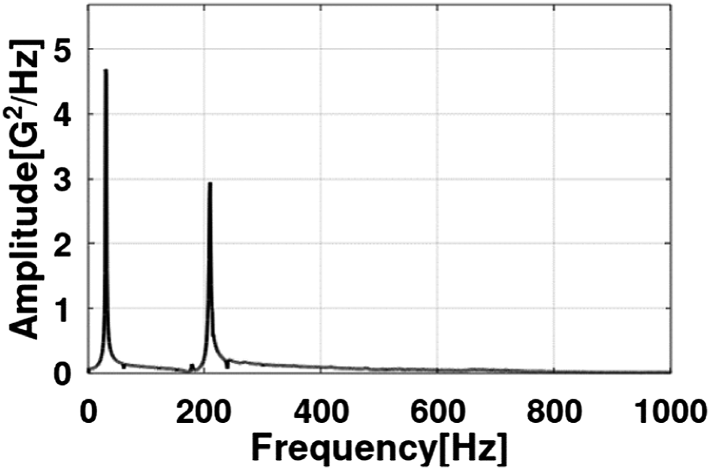
Numerical analyses for a small-scale supersonic jet and a clamped thin plate
Aero-acoustic prediction for a supersonic jet noise
A procedure for predicting the aero-acoustic loads generated from the supersonic jet is employed based on the RANS, DDES, and H-K methods. First, a three-dimensional RANS analysis is conducted to estimate the noise source of a supersonic jet flow. The computational domain is defined as 2.4 [m] for the nozzle axis and 1.6 [m] for the azimuthal direction. It is 120D e and 80D e in terms of the normalized exit diameter. The noise source can be located at a distance of 9-17 times the diameter of the nozzle exit. In addition, a steady flow region is chosen to utilize the H-K method, that is, the Kirchhoff surface location. In the current analysis, Kirchhoff surface is determined to be located within the region, where the static pressure may not vary by 0.7% with the atmosphere.
Second, a three-dimensional DDES analysis is employed for the supersonic jet noise in the near field, and the pressure variables for the H-K method located on the Kirchhoff surface. The cross-section of the present grid on the z = 0 plane is shown in Figure 11. In the present computational domain, the curved geometry of the supersonic jet is included. To resolve the turbulent flow from the wall, the first mesh size of the nozzle wall is 3 × 10⁻⁵D
e
, which is equivalent to the non-dimensional distance of 2. The mesh size is increased as the ratio of 1.2 along the radial direction. For the nozzle axis, the mesh size is chosen to be 0.01D
e
for the first grid spacing and increased with a ratio of 1.02. Furthermore, a fine mesh is also applied to cover the shear layer region. A cylindrical Kirchhoff surface is placed on the steady region obtained through a RANS simulation. The Kirchhoff surface is located within the region of 0 − 40D
e
for the nozzle axis and 10D
e
for the azimuthal direction. To store and transfer the pressure variables Cross section of the present grids on z = 0 plane.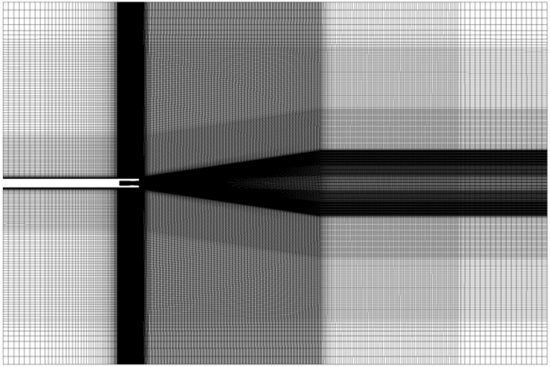
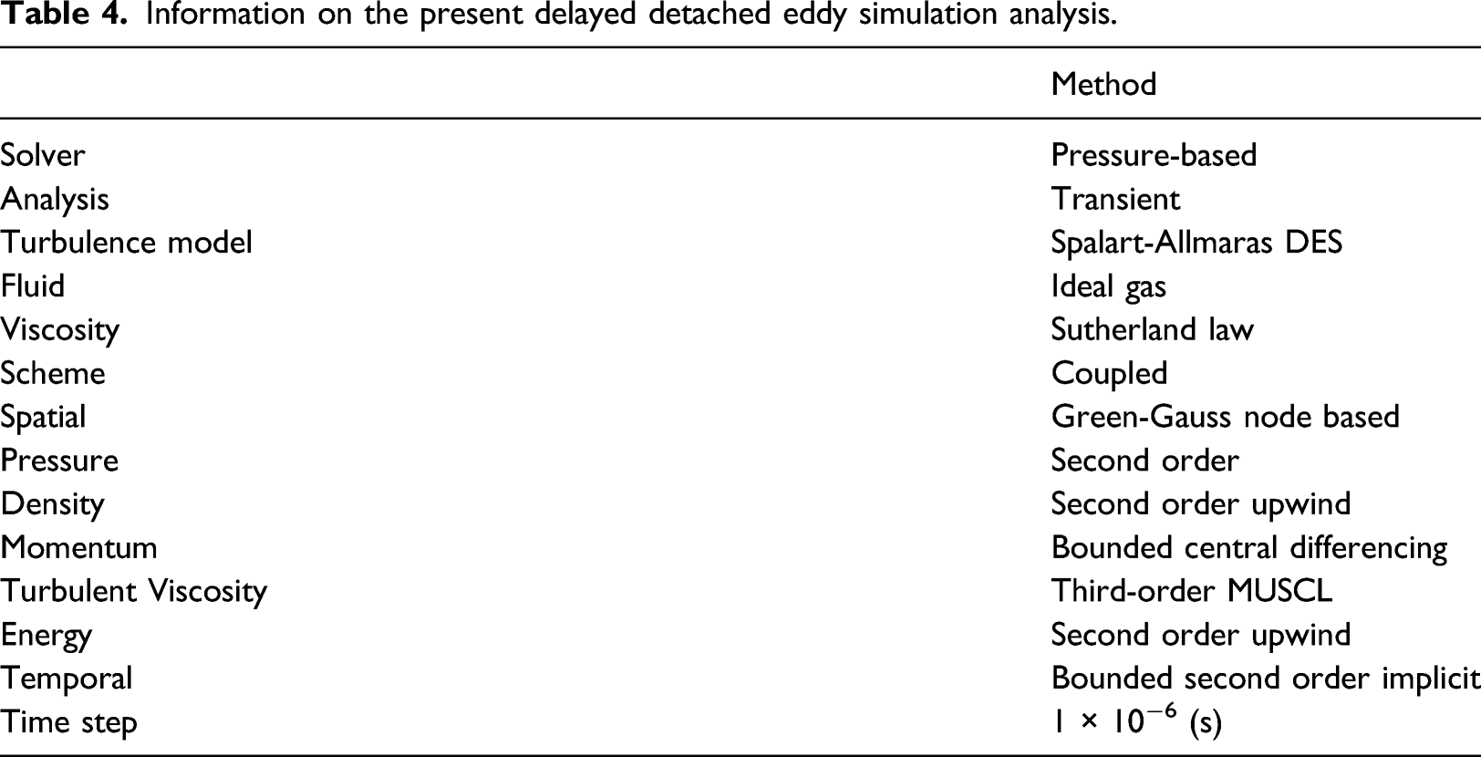
Information on the present delayed detached eddy simulation analysis.
Contour of the pressure for the present delayed detached eddy simulation analysis.
Vibro-acoustic analysis for a clamped thin plate
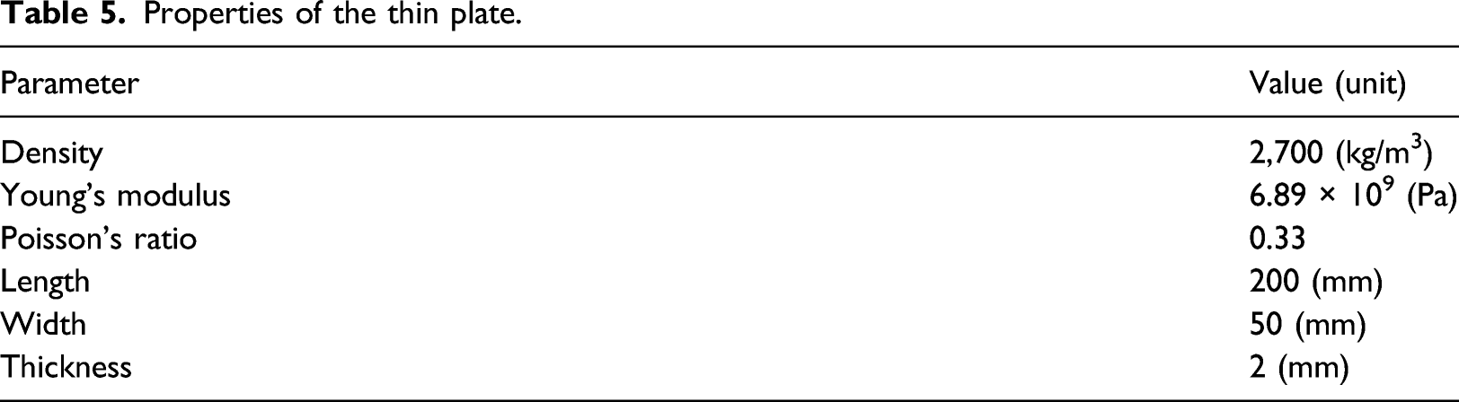
Properties of the thin plate.
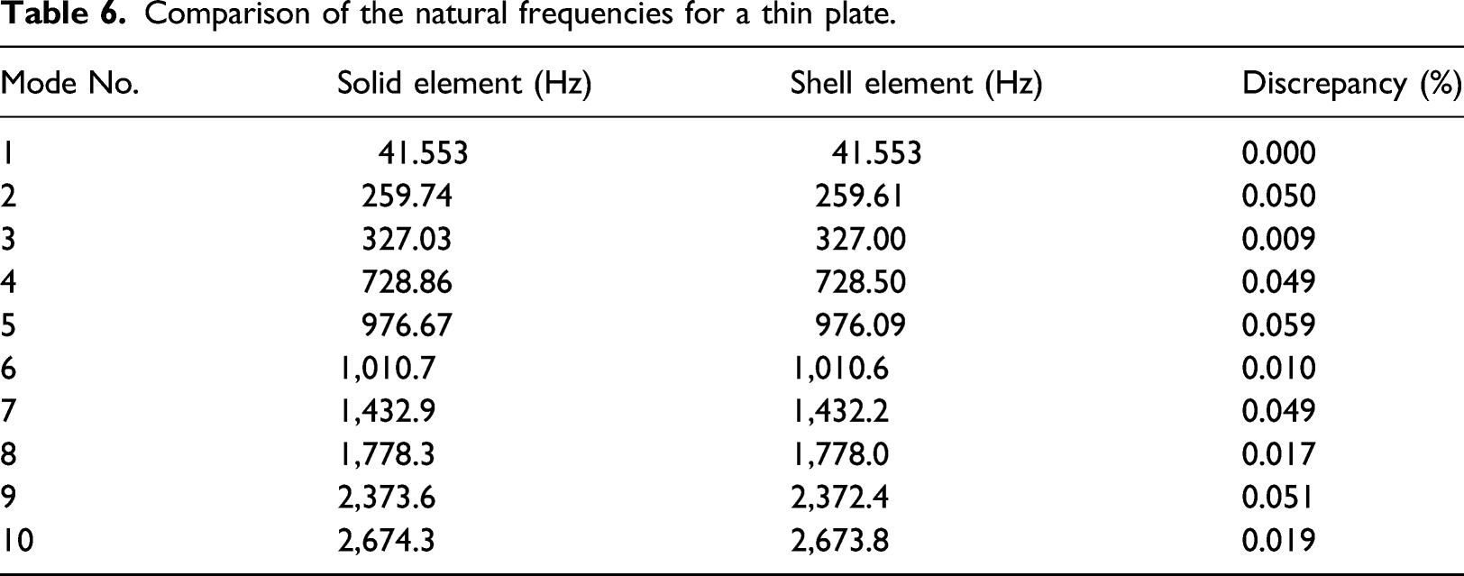
Comparison of the natural frequencies for a thin plate.
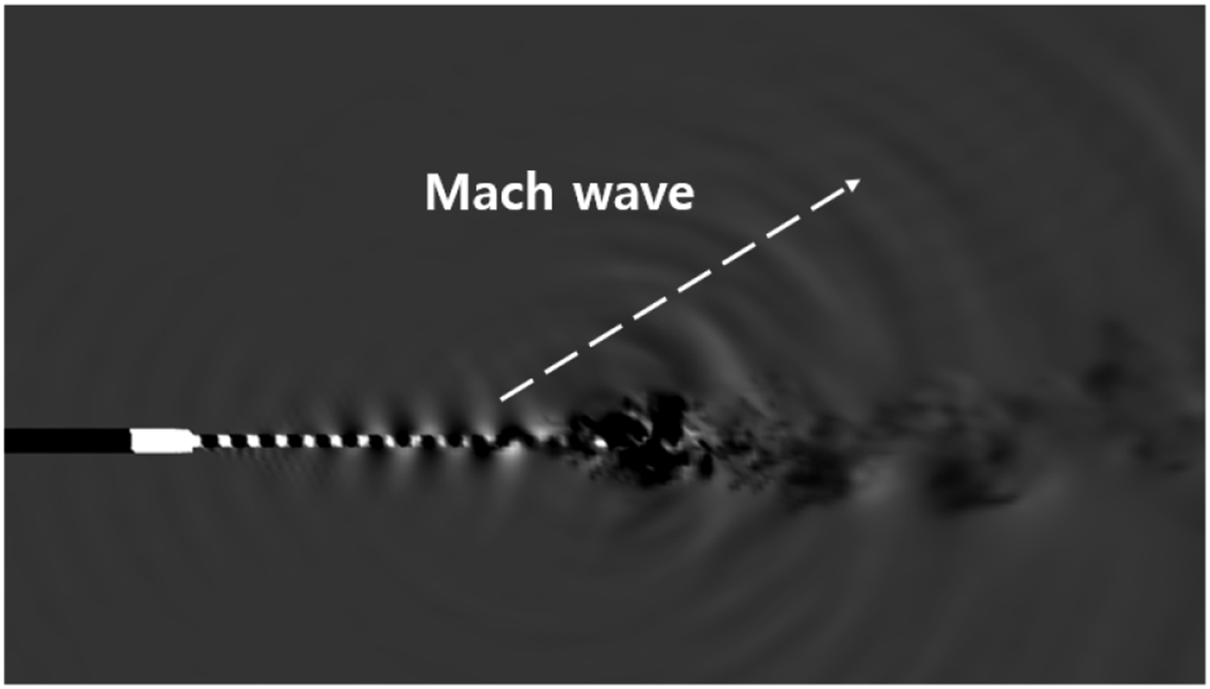
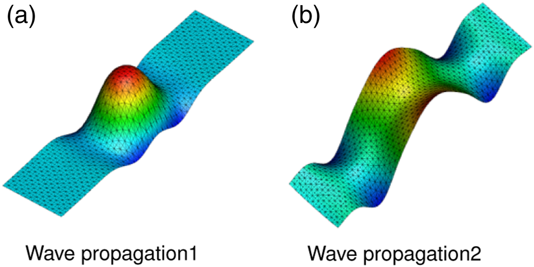
In the present FEM analysis, a transient acceleration is converted into the frequency and magnitude by employing a FFT and PSD. The reliable frequency range is dependent on the input signal, such as the sampling rate and duration. To investigate the FRF of the clamped thin plate, a unit step load is applied. Figure 13 describes the configuration of a clamped thin plate under a unit step load and receiver. Without damping, the waves generated by the unit step load propagate and finally excite the clamped thin plate with their own natural frequencies. Figures 14(a) and (b) show two images of the wave propagation on the plate. Impact load on a clamped thin plate. Wave propagation in a clamped thin plate.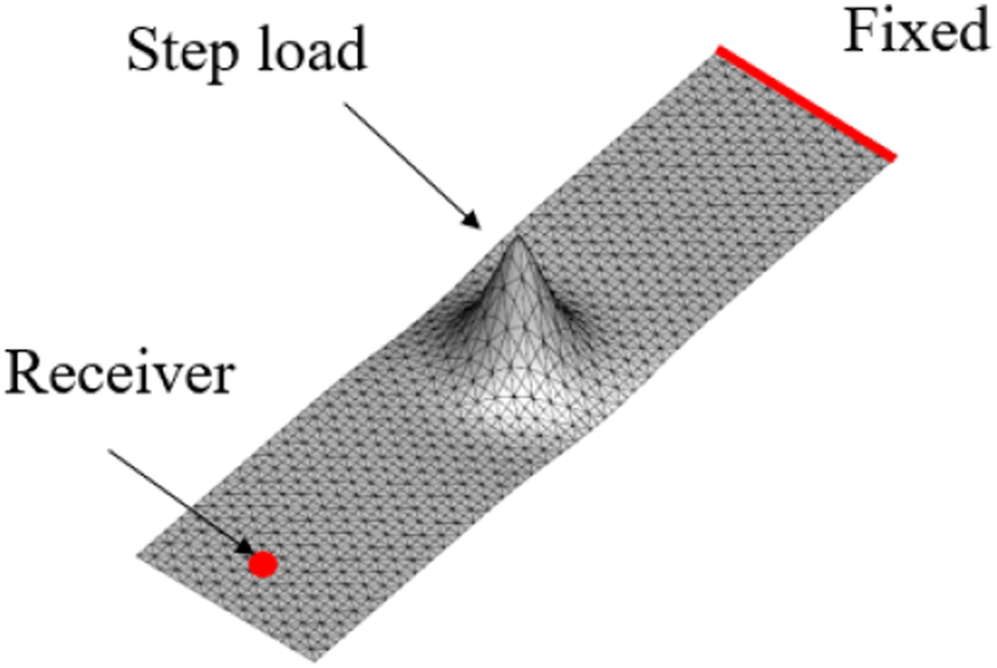
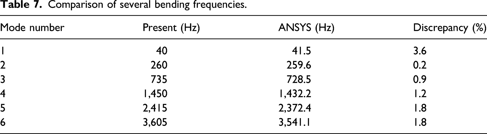
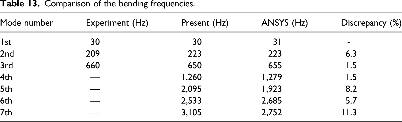
To estimate the natural frequencies of the present plate, the transient acceleration at the receiver is transformed into the frequency domain by applying the FFT. The total numbers of nodes and elements are 6,601 and 12,800, respectively. The time step (Δt) is chosen as 10−5 [s] and the elapsed duration (T) is 0.2 [s]. Hence, the frequency resolution (Δf) and maximum reliable frequency (fmax) are 5 [Hz] and 50,000 [Hz], respectively.
Comparison of several bending frequencies.
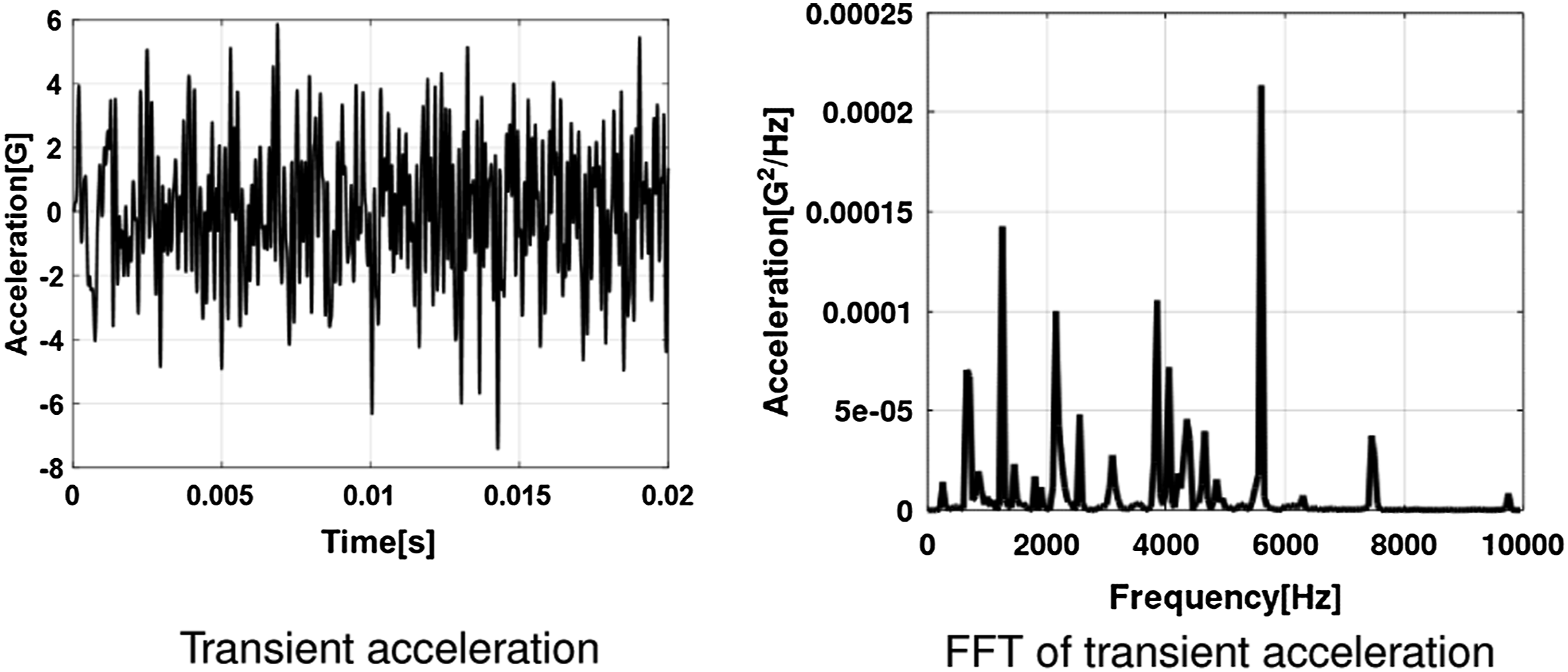
Finally, a vibro-acoustic analysis was conducted to predict the structural responses owing to the aero-acoustic pressure generated from a small-scale supersonic jet. The transient acoustic pressure applied on a clamped thin plate is predicted by combining both the DDES and the H-K method. Based on the numerical results obtained by DDES analysis, the transient acoustic pressure can be predicted by propagating the acoustic pressure from the H-K surface. Figure 15(a) shows the transient pressure history applied to structures at Position 1, as shown in Figure 9. Sequentially, the transient acceleration is obtained by conducting a transient FEM analysis with the transient pressure as shown in Figure 16(a). Transient pressure and fast Fourier transform at Position 1 Transient acceleration and fast Fourier transform at Position 1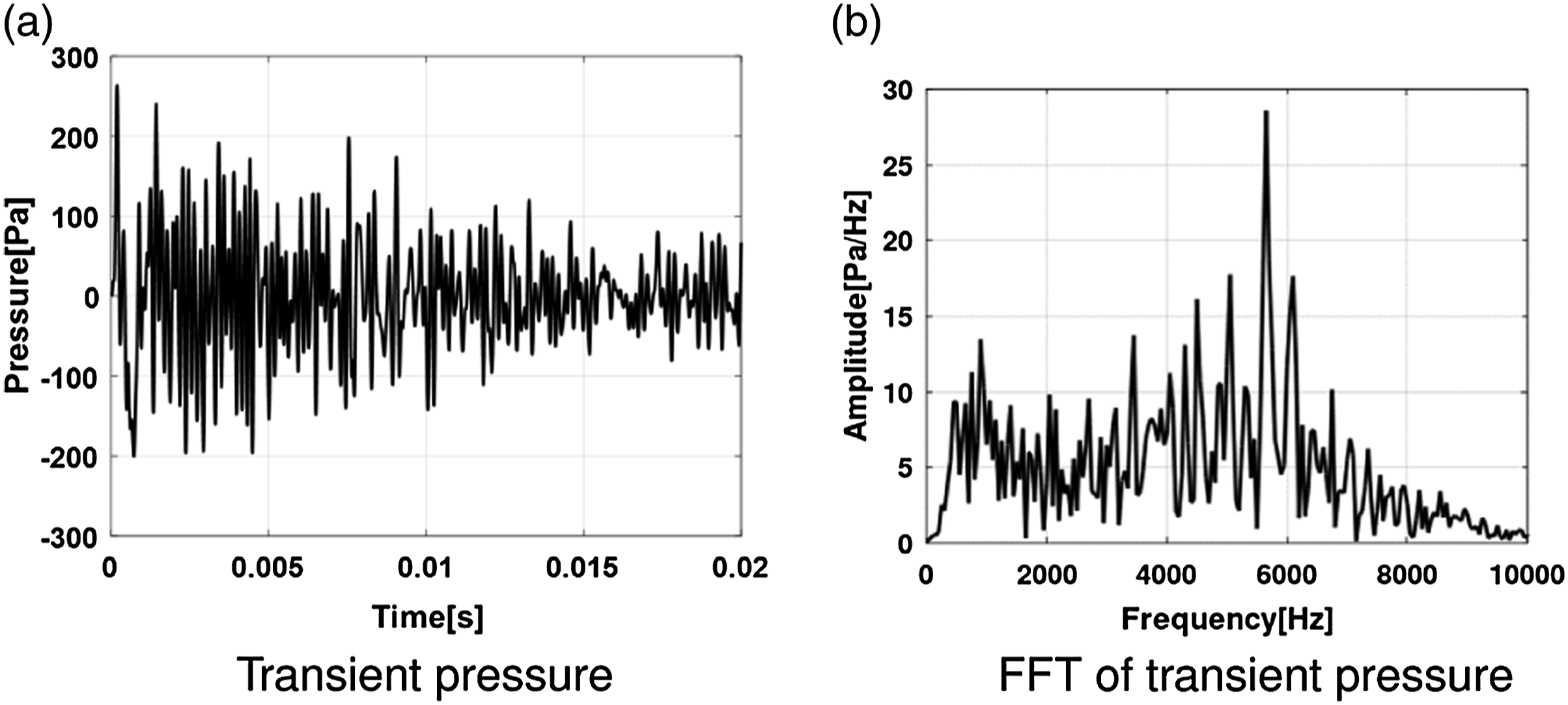
Prediction and validation for a small-scale supersonic jet and a clamped thin plate
The objective of this study is to verify present aero-vibro-acoustic analysis procedure for the aero-acoustic loads generated from a small-scale supersonic jet and the vibro-acoustic response of a clamped thin plate. First, the numerical results of the RANS and DDES analyses are compared with those obtained by previous studies. Second, the supersonic jet noise is predicted and further validated with experimental results at both the near and far-fields. Third, equivalent modeling for an FEM analysis is presented to consider the decreased natural frequencies found in the experiment owing to the mass of the accelerometer. Fourth, APSDs for a clamped thin plate at three different locations are validated with the values obtained by experimentally.
Validation of RANS and DDES analysis
An understanding of the shock-cell structure of the supersonic jet flow field indicates that aeroacoustic behavior is significantly contributed to by the shock. The shock-cell length given by the experimental measurement
22
and that by Prandtl’s vortex sheet model
23
are compared in Figure 17. The first three shock cells are used owing to the limitation that the vortex sheet model is only valid in the initial region of the supersonic jet. Equation (2) is Prandtl’s vortex sheet model in the form of the supersonic jet Mach number (M
j
) and exit diameter (D
j
). The present shock-cell spacing is 1.88D
e
with an exit Mach number of 1.8. The comparison between the present results and the previous LES analyses shows good agreement, whereas the empirical model overpredicts the shock cell length. Shock-cell spacing versus the supersonic jet Mach number.
Furthermore, the centerline pressure decay of the supersonic jet was also compared with that obtained in a previous study.
24
The centerline pressure decay of three different nozzle pressure ratios (NPRs) is presented in Figure 18. The pressure fluctuates significantly and decreases along the centerline owing to the oblique shock. The shock-cell length of NPR 6.41 is located between those of NPRs 6 and 7 obtained by the experimental measurements. However, the centerline pressure for NPR 6.41 is overpredicted by the present DDES analysis as compared with the experiments for NPR 6 and 7 after the end of the potential core, which is located at roughly 15.88D
e
. The phenomena of the overpredicted centerline pressure have been reported in previous studies as well.25,26 Centerline pressure decay of the jet at nozzle pressure ratio of 6, 6.41 and 7
Validation of the supersonic jet noise at near and far-fields
The supersonic jet noise prediction was validated with the experimental results. For the numerical analysis, the near-field noise prediction can be achieved by utilizing CFD numerical results without the H-K method because it is located within the Kirchhoff surface (10D
e
). To extract the acoustic noise from the numerical results, the static pressure is stored while the DDES analysis is in progress. By applying the root mean square (RMS) technique, OASPLs of 12 locations in the near-field are obtained and compared with those obtained experimentally. Figure 19 shows a comparison of the OASPLs between the numerical and experimental results. A fifth-order Butterworth filter with a range of 500–9,600 [Hz] is employed. Details are provided in Table 8. The average discrepancy is 4.09 [dB] for 12 locations of a linear array. The maximum and minimum discrepancies are 8.63 [dB] at 0D
e
and 0.4 [dB] at 20D
e
, respectively. Although the averaged OASPL’s along the distance from the nozzle exit are similar to each other, the OASPLs are overpredicted by the numerical analysis from 0D
e
to 15D
e
. Comparison of the overall sound pressure level at the near-field for the supersonic jet. Overall sound pressure level at the near-field for the supersonic jet.
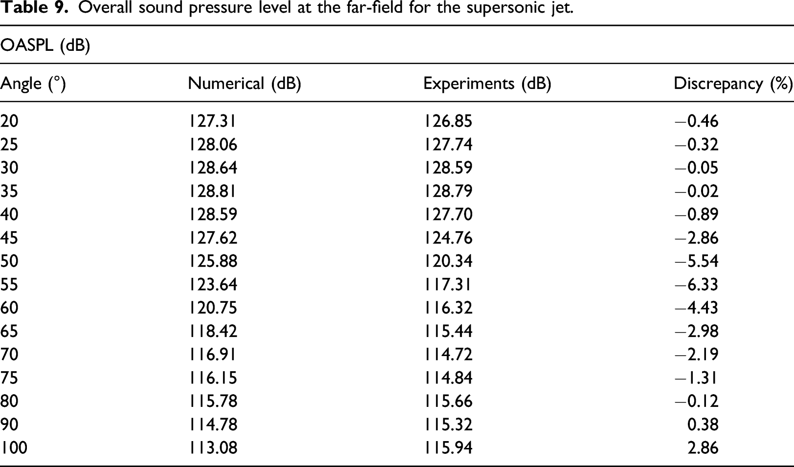
Similarly, the far-field noise prediction is obtained from the H-K method by projecting the accumulated numerical results to the far-field location. Although the turbulent flow, including the frequency characteristics, is contained in the DDES analysis, inter-point interval of Kirchhoff surface is carefully considered. In the current analysis, the static pressure and spatial/temporal derivatives are stored at a large capacity storage for every ten time steps (1 × 10⁻⁵ [s]) at 23,040 points. The inter-point interval was chosen to be 0.005[m], and the reliable maximum frequency was 9,600 [Hz]. Figure 20 shows the OASPLs along the varying angle from the noise source. More details are summarized in Table 9. The average discrepancy is 2.05 [dB] for 15 locations of the annular array. The maximum and minimum discrepancy are 6.3 [dB] at 55° and 0.02 [dB] at 35°, respectively. Comparison of overall sound pressure levels at the far-field for the supersonic jet. Overall sound pressure level at the far-field for the supersonic jet.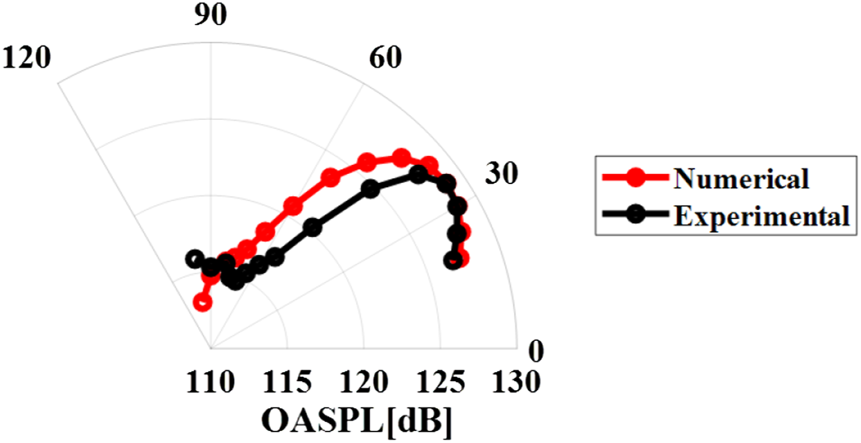
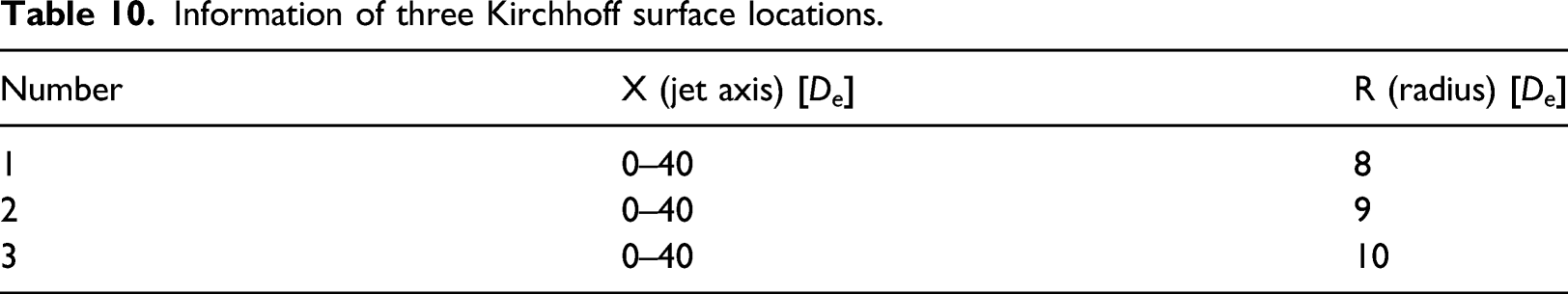
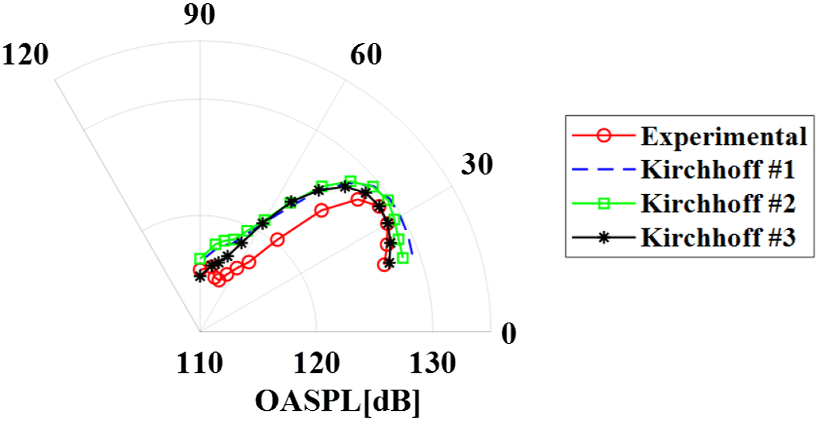
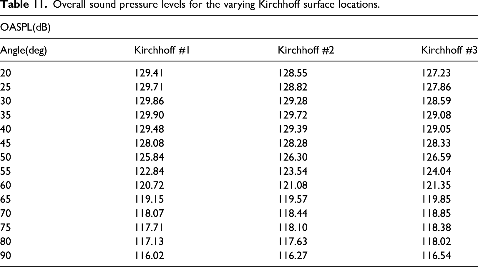
To find an effect of Kirchhoff surface location, three different Kirchhoff surface locations are employed as shown in Figure 21. The information about the three Kirchhoff surface locations is also given in Table 10. The tendency in Figure 22 and Table 11 shows good agreement for all the range while those at 20° are decreased as Kirchhoff surface is far from the supersonic jet noise source. Three different Kirchhoff surface locations. Information of three Kirchhoff surface locations. Comparisons of the overall sound pressure levels at the far-field for three different Kirchhoff surface locations. Overall sound pressure levels for the varying Kirchhoff surface locations.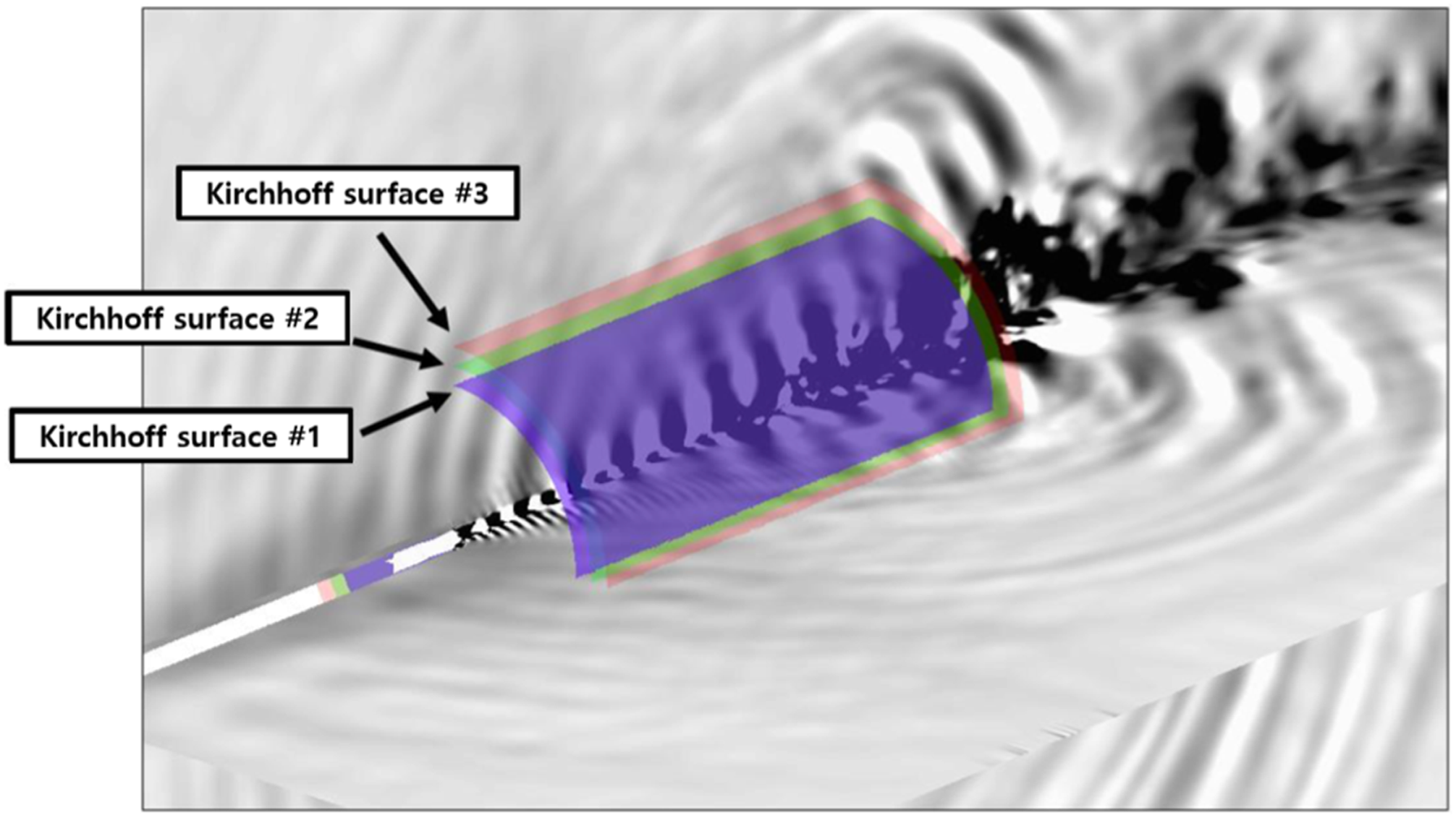
From the numerical results for the near-field, OASPLs are overpredicted within a range of 0-20D
e
compared to those obtained by the experiments. In addition, the OASPLs of the numerical results for the far-field overpredict at angles of greater than 40°. As shown in Figure 23(a), the near-field can be divided into two regions: large-scale structure (LSS) and fine-scale structure (FSS) dominant regions. When the noise source of the supersonic jet is assumed to be located at 9D
e
, the measured point at Simplified scheme for both near-and far-field array.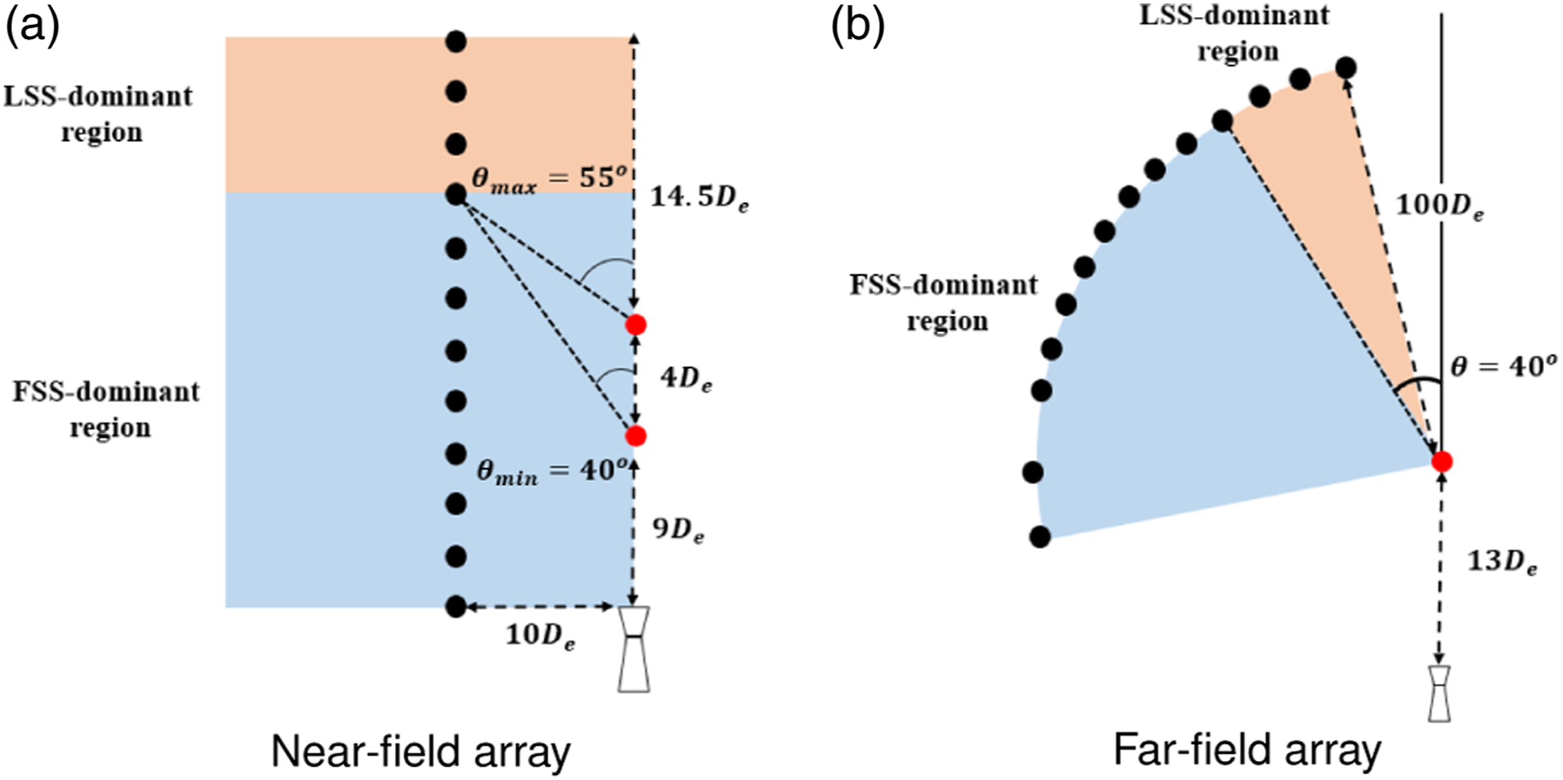
The discrepancies between OASPLs and PSDs are compared in the LSS- and FSS-dominant regions for the near and far-fields. Figure 24 shows the PSDs of the near-field at x = 0D
e
, 10D
e
, 20D
e
and 25D
e
. It is shown that the PSD values are overpredicted within the range of 0-10D
e
, whereas they are similar for the range of 20-25D
e
. In addition, PSDs of over 6,000 [Hz] or greater decrease along with the FSS-dominant region. The resolved frequencies may vary with the computational location owing to the coarse meshes. The peaks are measured for the range of 20-25D
e
and 20° < θ < 40° as shown in Figures 24(c)-(d) and 25(a)-(b), respectively. It is because the measurement position is close to peak radiation angle assumed to be 35°. Comparison of power spectral densities for the near-field. Comparison of power spectral densities for the far-field.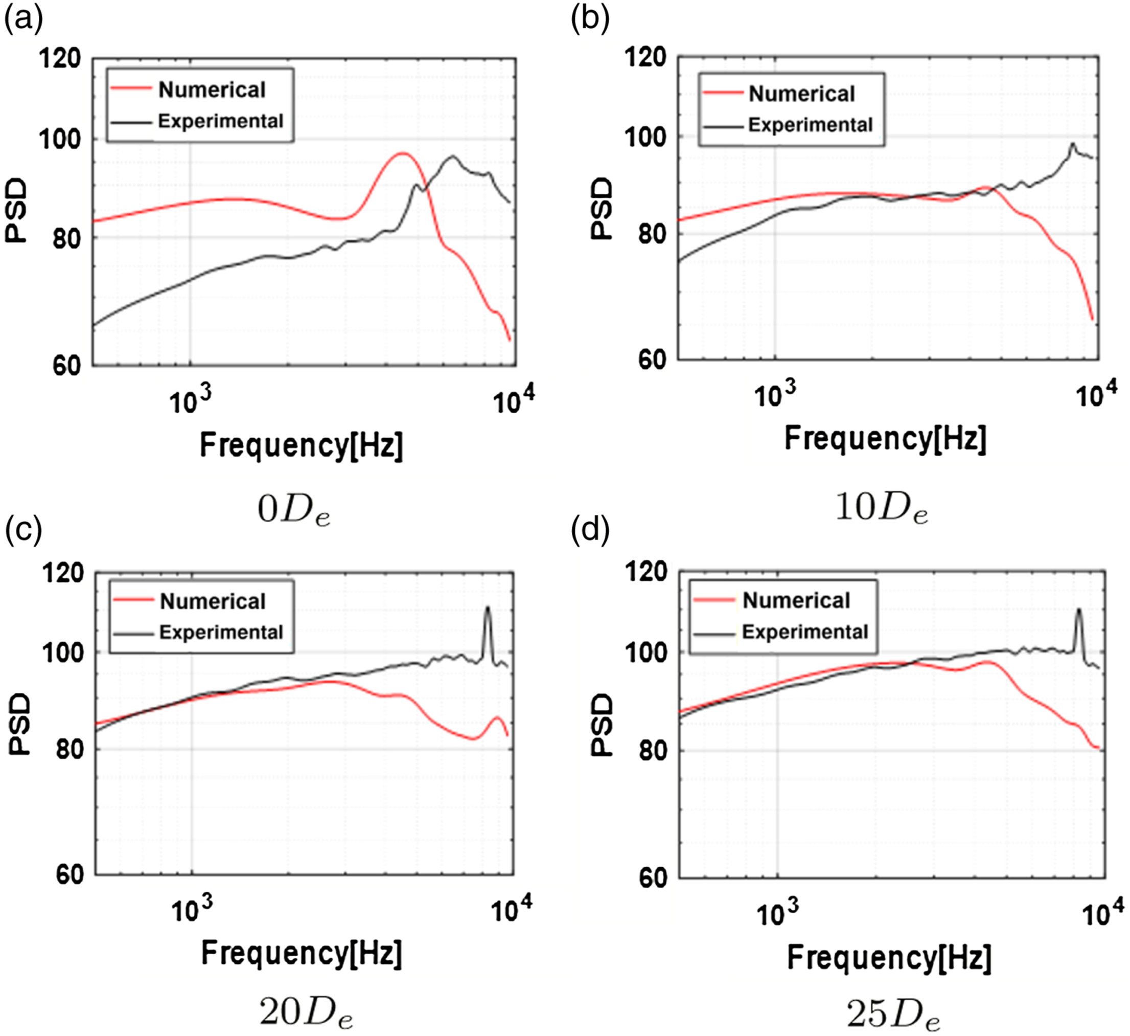
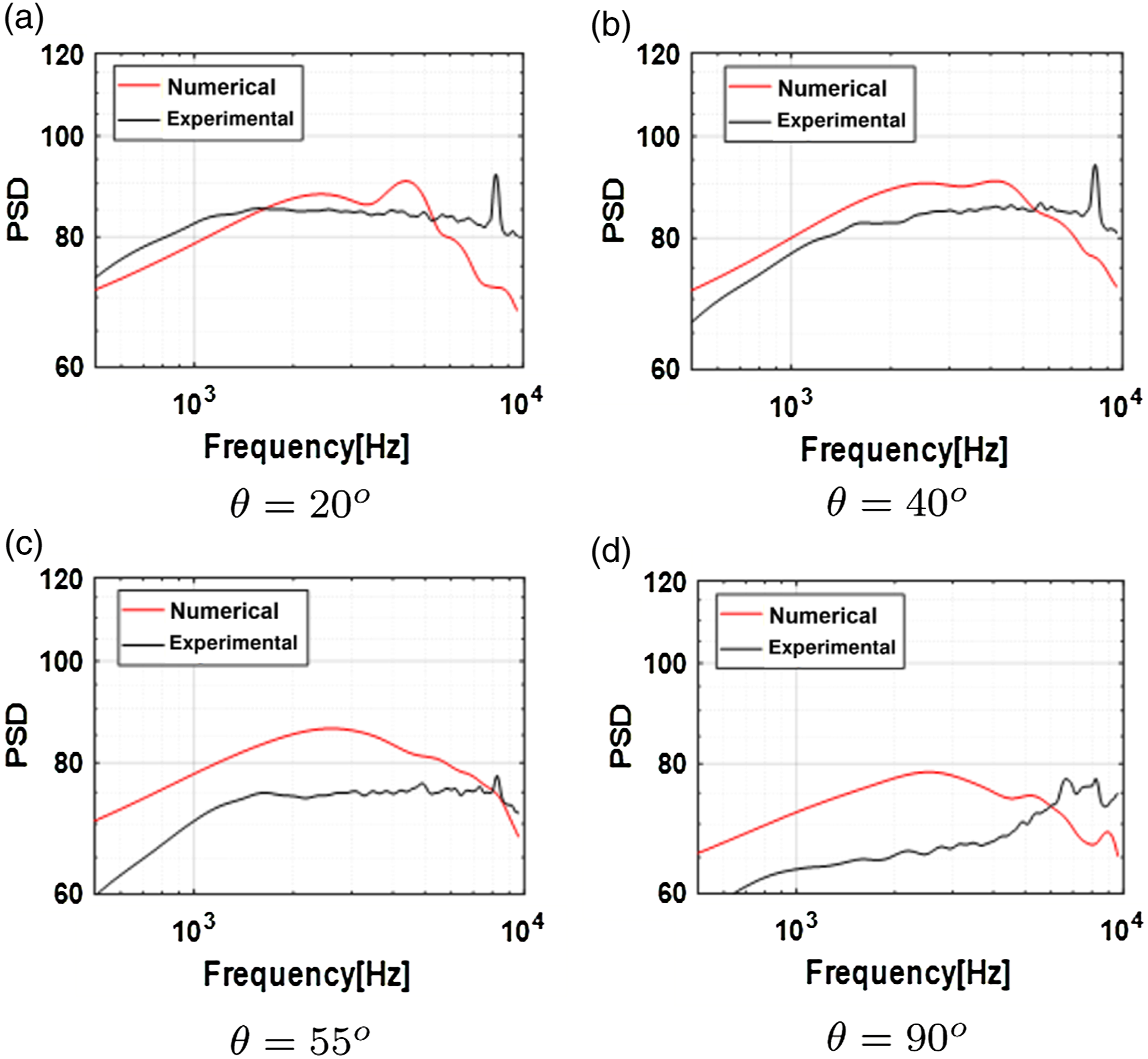
Figure 25 depicts the PSDs of the far-field at θ = 20°, 40°, 55° and 90°. It is also revealed that PSDs are overpredicted at θ = 55° and 90°, whereas those are similar at θ = 20° and 40°. From the comparison, the present DDES analysis predicts the PSDs and OASPLs within the LSS-dominant region, whereas those of the FSS-dominant region are overpredicted.
An over-predictive tendency for a supersonic jet noise prediction was also reported in previous studies. Labbe et al. 26 developed computational fluid dynamics/computational aero-acoustics (CFD/CAA) in which OASPLs were overpredicted in the FSS-dominant region (θ > 45 o ). The spatial discretization method is based on the finite volume method (FVM) on a structured grid, similar to the present DDES analysis methodology. Fukuda et al. 27 employed an implicit LES for a solid rocket in static firing based on the finite difference method (FDM). At over a 50° angle from the jet axis, the OASPLs were overpredicted. Liu et al. 28 investigated an under-expanded supersonic jet with a design Mach number of 1.5 based on the FEM. The near- and far-field OASPLs showed a similar trend: noise prediction in the LSS-dominant region showed agreements, whereas those in the FSS-dominant region were overpredicted. Although different discretization schemes are employed in the aforementioned studies,26–28 an over-predictive tendency is similarly observed in the FSS-dominant region. In addition, the number of azimuthal grid points is less than 160 in both previous studies and the current analysis. If the resolution of the computational grid is insufficient to resolve the high frequency, the SPL is generally overestimated. This is induced by a higher energy at lower frequencies than the physics from the turbulent structure of the jet shear layer. When the azimuthal grid points are coarse, the RMS values of the axial and radial fluctuating velocities are overestimated. Hence, the RMS values of the fluctuating pressure are also estimated. From the effects of the azimuthal grid resolution conducted by Nonomura et al. 29 and Bogey et al., 30 the OASPL values decreased with the use of 1,024 grid points compared with those obtained by 256 grid points in the FSS-dominant region. This indicates that the overestimated PSD has a significant impact on the FSS-dominant region because the SPL of the low-frequency structures are relatively smaller than those in the LSS-dominant region. In conclusion, the present DDES analysis with the second order in time and space may predict OASPL’s accurately at LSS-dominant region, whereas the number of azimuthal grid points needs to be increased to accurately predict the FSS-dominant region.
Equivalent modeling for FEM analysis
Comparison of the natural frequencies with/without an accelerometer.
Comparison of the bending frequencies.
Validation of the present vibro-acoustic analysis
Figure 26 presents unfiltered and filtered APSDs acquired at Position 1 from the experiment. It was found that the noise is included in the finite results. For the experimental noise reduction, Welch’s method is employed using a window length and sampling rate of 12,800 and 50 [%], respectively. Acceleration power spectral densities for the experiment at Position 1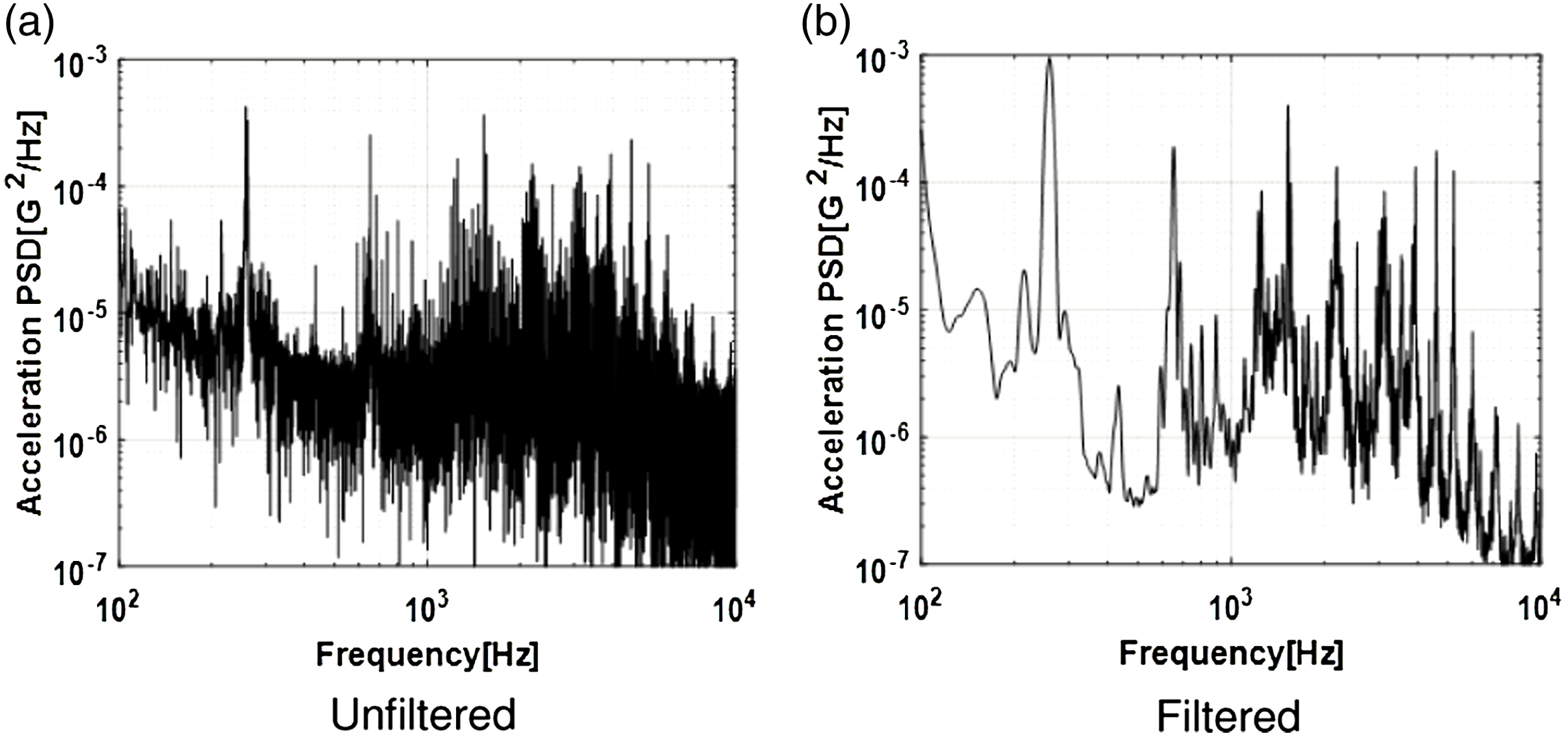
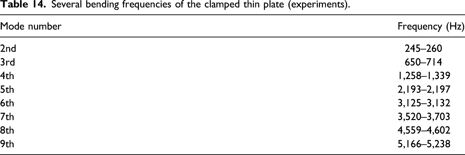
APSDs for three different positions, Positions 1-3, are obtained by the accelerometer in Figure 27. The magnitude of the APSD at Position 2 is larger than that measured at Positions 1 and 3. In addition, it was found that the APSD at Position 3 is much smaller than the others owing to the low amplitude of transient pressure. However, the natural frequencies of a clamped thin plate are determined by comparing the peak amplitudes of the APSDs at three different locations. Table 14 lists the bending frequencies of the clamped thin plate obtained through the experiments. The remaining peak frequencies at 1,526 [Hz] and 2,533 [Hz] are assumed to be the bending-related frequencies. Comparison of acceleration power spectral densities at three different positions. Several bending frequencies of the clamped thin plate (experiments).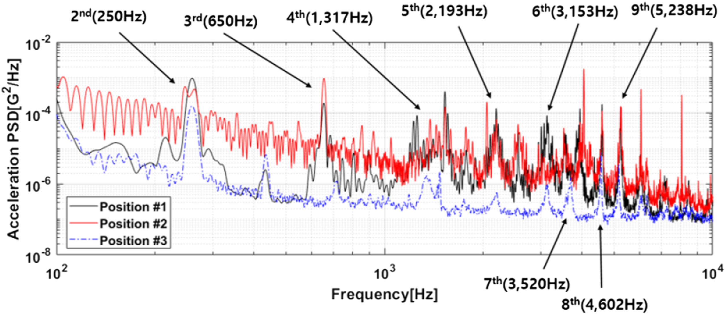
For the numerical analysis, the transient pressure history is obtained by the propagating pressure wave based on the H-K method. The transient pressure at 0.02 [s] is extracted owing to the limited elapsed duration of the DDES analysis. Finally, a vibro-acoustic analysis is conducted by using the transient pressure and the transient FEM analysis. The frequency range of the APSDs is divided into the following two regions: 1) 100-1,000 [Hz] for the lower frequency and 2) 1,000-5,000 [Hz]. Figure 28 compares the APSDs for the numerical and experimental results at Position 1. The second and third bending frequencies were found to be 250 and 650 [Hz], respectively, as shown in Figure 28(a). In addition, the magnitude of the APSD in the numerical results from 300 to 1,000 [Hz] is similar to those obtained through the experiments. In Figure 28(b), the bending frequencies from the fourth through sixth modes are similar, whereas higher bending frequencies obtained through the numerical results are decreased when compared with those obtained experimentally. Comparison of acceleration power spectral density at Position 1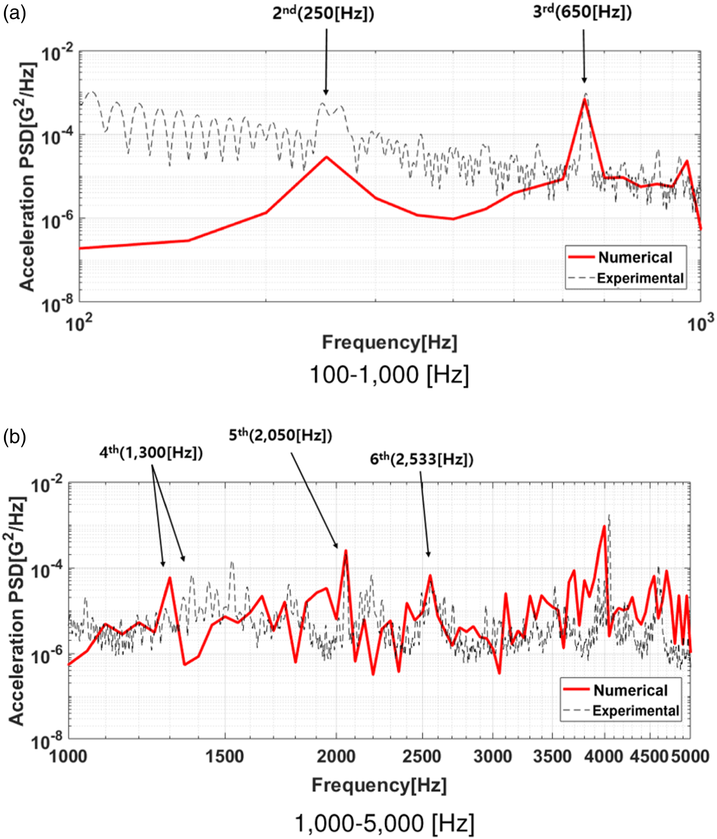
In a similar manner, the APSDs of both the numerical and experimental results at Position 2 are described in Figure 29. The magnitude of the APSD for the numerical results at 250 [Hz] is smaller than that for the experimental results. This is caused by a lack of elapsed duration for the simulation in the current analysis. The magnitudes of the APSD at 650 [Hz] are approximately 0.001 [G2/Hz] and the current analysis is capable of accurately predicting the lower frequencies. In Figure 29(b), the fourth bending frequency is found to be 1300 [Hz] based on the numerical analysis and 1,377 [Hz] during the experiments. The fifth and sixth bending frequencies are similar to each other. However, the higher bending frequencies obtained by the numerical analysis are smaller than those obtained by the experiments. Comparison of acceleration power spectral density at Position 2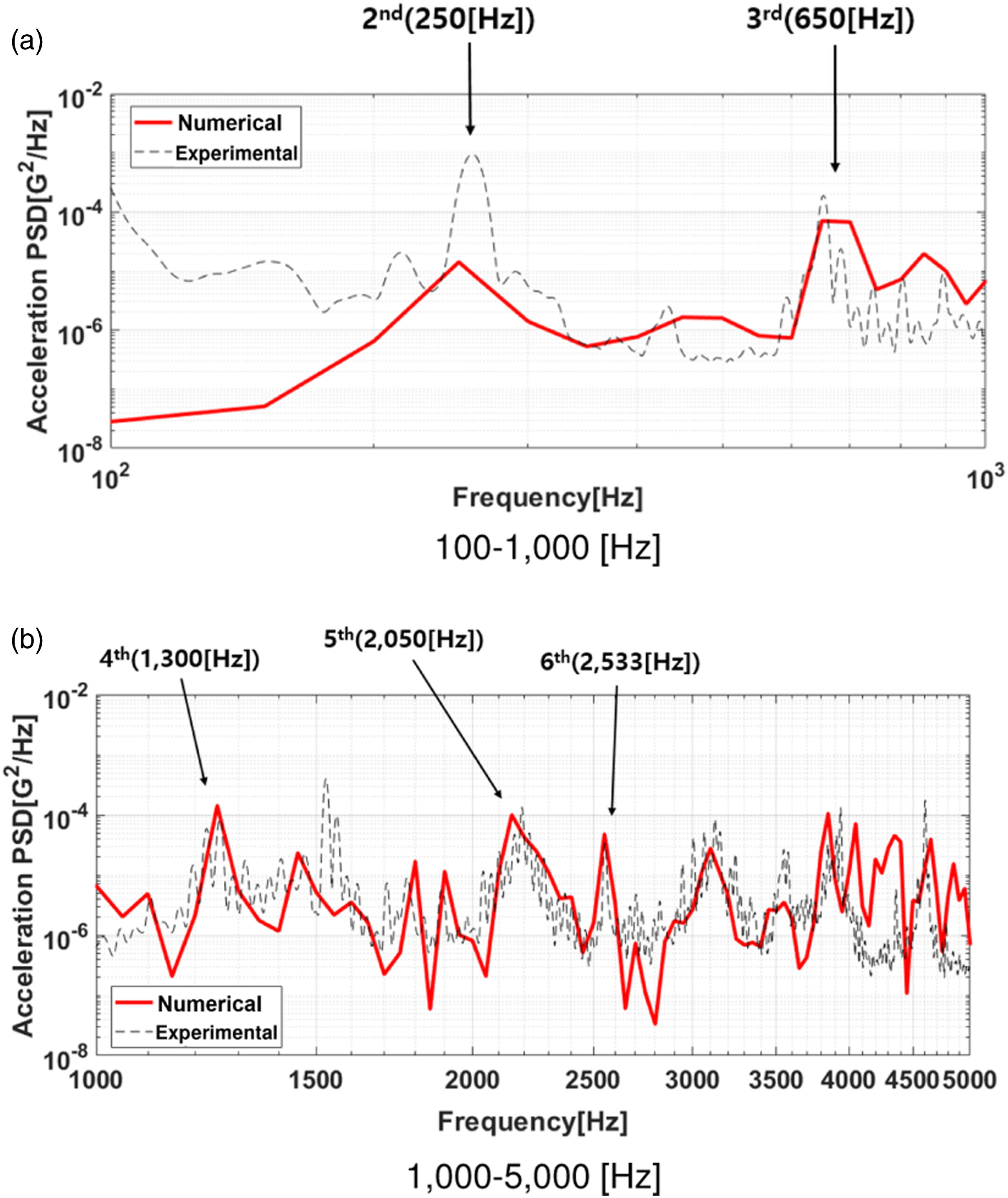
Figure 30 describes APSDs of both numerical and experimental results at Position 3. The magnitude of the APSD for the numerical results at 250 [Hz] is much smaller than that for the experimental results. However, The magnitude of APSD at 650 [Hz] is greater than that of experiments. Whereas the APSDs of both the numerical and experimental results are of similar magnitude, a numerical analysis is not capable of predicting the natural frequencies of a clamped thin plate. Only the fourth bending frequency is obtained through the numerical analysis. Comparison of acceleration power spectral density at Position 3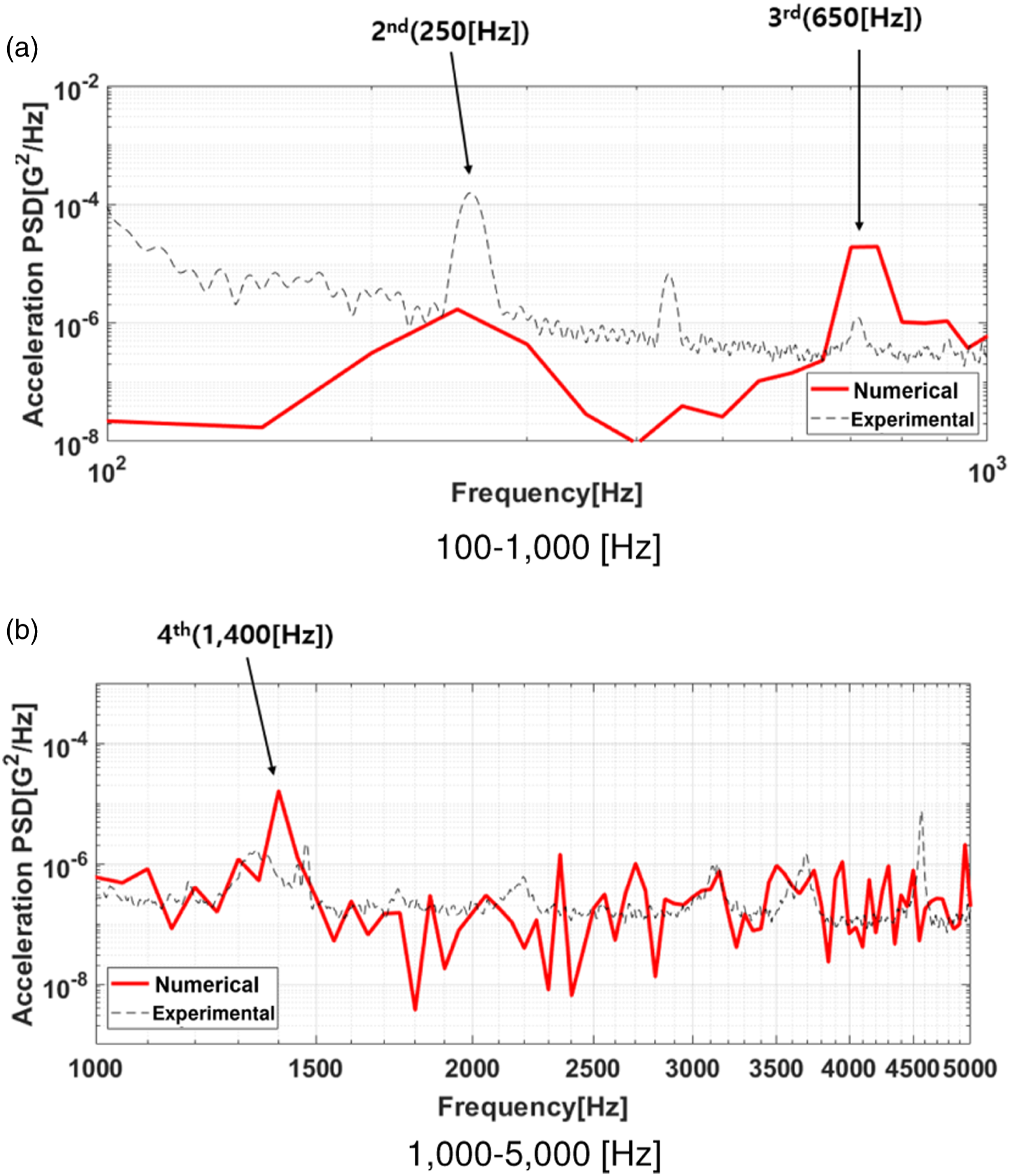
To summarize the present FEM analysis is capable of predicting several natural frequencies for a clamped thin plate vibrated using aero-acoustic loads obtained by DDES and H-K method. Whereas the APSD at only Position 3 obtained by the current analysis is of similar magnitudes, the APSDs at both Positions 1 and 2 are correlated with better magnitudes and natural frequencies. This suggests that APSDs of a clamped thin plate are dependent not only FEM modeling but also on the aero-acoutsic characteristics such as the pressure magnitudes, distance and orientation angle from the noise source.
Conclusion
A sequentially integrated aero-vibro-acoustic procedure was developed to predict the OASPLs of a small-scale supersonic jet at the near- and far-fields and APSDs of a clamped thin plate vibrated using aero-acoustic loads. Experiments using a small-scale supersonic jet were conducted as well. An aero-acoustic prediction was applied by employing DDES and H-K method. The near- and far-field noise predictions were presented and further compared with those obtained by experimental results. Due to the low-discretization in space and time and coarse meshes in the higher-angle area (θ > 45°) from the supersonic jet noise source, overestimated numerical results were acquired at the FSS-dominant region. However, OASPLs at the LSS-dominant region were accurately predicted by the present DDES and H-K analysis. A vibro-acoustic analysis was also conducted based on the FEM analyses. The transient pressure was predicted by the propagating pressure wave based on the H-K surface. In addition, three different APSDs of a clamped thin plate were presented and further validated with those experimentally obtained. Although the magnitudes and peak frequencies for the lower-frequency range were nearly equal to those determined through the experiment, there is still ambiguity in higher-frequency bands where hybrid FEM/SEA or SEA should be employed. However, it is found that an integrated aero-vibro-acoustic procedure is capable of predicting the OASPLs of a small-scale supersonic jet and APSDs of a clamped thin plates. In near future, higher-order in space and time will be adopted for improvement of the CFD analysis. Furthermore, hybrid FEM/SEA will be also employed in order to predict vibro-acoustic characteristics in high-frequency range.
Footnotes
Acknowledgements
This work was conducted at High-Speed Vehicle Research Center of KAIST with the support of the Defense Acquisition Program Administration and the Agency for Defense Development under Contract UD170018CD. The authors thank Kent L. Gee for helpful advice on jet noise measurements.
Declaration of conflicting interests
The author(s) declared no potential conflicts of interest with respect to the research, authorship, and/or publication of this article.
Funding
The author(s) received no financial support for the research, authorship, and/or publication of this article.