






Abstract
Defect and damage identification is a crucial task in structural health monitoring (SHM) systems. Recent advances in deep neural networks (DNNs) show success in identification from data for a wide range of SHM systems. However, this approach faces challenges in terms of robustness and scalability with respect to data scarcity. Data collection for the training of DNNs from both the field and laboratory experiments is costly. To address this issue, we employ transfer learning (TL) through the use of deep convolutional neural networks (CNNs) for defect identification in the context of a sensor network’s vibration data. A deep TL (DTL) paradigm is used herein so that a pretrained CNN, primarily trained for generalized defect identification tasks where sufficient training data exist (source domain), can be re-trained partially (fine-tuned) as a later secondary process that targets this application domain (target domain) specifically. Different DTL cases are compared, and training data are enhanced with numerical simulation data. The efficacy and robustness of this method are demonstrated on defect identification for full-scale prefabricated concrete shear wall structures with different levels of data scarcity. This method utilizes dynamic responses collected using a sensor network. This is an extension of deep learning vision for non-vision tasks. Defect features are extracted from the dataset of dynamic responses using this DTL frame. Experimental results show that this approach can improve identification models on datasets with few samples.
Keywords
Introduction
Steel sleeve grouting connection technology is commonly used for the steel bars of beams, columns, and shear walls in prefabricated buildings. However, grouting defects form easily, reducing the stability of components and structures, and affecting the connection quality and structural safety. Therefore, the quality inspection of steel sleeve grouting connections is particularly important.
A steel sleeve grouting connection includes a ribbed bar, sleeve, and grouting made of materials including cement, fine aggregate, and concrete admixture. 1 Fluid grouting has good fluidity, early and high strength, and micro-expansion. When constrained by a sleeve, a large positive stress is generated between the solidified grouting and the sleeve. Friction force is generated on the ribbed bars, transmitting axial stress. An insufficient grout sleeve will affect the axial force transmission of the ribbed bars, and hence the seismic performance and safety of a structure.2,3 To detect the fullness of sleeve grouting is a challenge, since it is not visible and has a complex internal structure.
Conventional methods to identify connection defects in prefabricated structures include embedded testing (embedded sensor and embedded wire drawing), 4 core drilling, 4 and non-destructive testing (X-ray; ultrasonic wave; impact-echo, ground penetrating radar-based testing).5,6 These methods face challenges that make then inconvenient for large-scale field application. Embedded testing requires embedded detection elements, and can only detect grouting quality near the embedding site. Core drilling will damage the structure. Ray- and wave-based methods tend to be laborious and costly, and their applications are often limited due to the complexity of the connection. 7
Deep learning-based defect identification methods have attracted much attention,8,9 especially as related to images,10,11 as a natural application of deep learning (Bao et al., 2019). 12 Yeum et al. 13 applied convolutional neural networks (CNNs) to structural collapse classification using collected post-disaster images, Dung 14 used them to detect cracks in concrete structures, and Xu et al. 15 applied them to seismic damage identification of reinforced concrete columns. These methods only apply to defects and damage that can be visually detected.
For interior and invisible defects, vibration signals are relatively easily collected, and have been used to analyze identification problems as an extension of deep learning vision.16,17 Deep learning methods can automatically extract features from original data, avoiding the extraction of fixed features in the early stage. Deep learning has shown great potential in complex structural defect identification, where traditional feature-based classification is difficult. Jiang et al. 18 proposed a multiscale CNN architecture using vibration signals for wind turbine gearbox fault diagnosis. Zhang et al. 19 proposed a one-dimensional CNN to detect changes in structural stiffness and mass. Kumar et al. 20 applied CNNs to defect identification of bearings based on vibration signals. These deep learning-based methods rely on massive labeled training datasets in a complex, complete, end-to-end feature extraction, representation, and classification process. To collect structural vibration signals in the field of civil engineering is expensive and time-consuming, which brings a challenge to deep learning-based non-destructive defect identification.
Transfer learning (TL) is an important technology in machine learning for solving data scarcity problems, 21 and therefore, a TL paradigm via the use of a deep CNN provides a new idea for defect identification in the case of insufficient test data. 22 The datasets of the source and target domains of TL can have different probability distributions, making deep learning more robust. 23 Xu et al. 24 (2020) proposed an inter-class knowledge transfer-based structural damage identification meta-learning paradigm. Wu et al. 25 proposed a structural crack detection method based on a CNN and TL. The efficiency and transfer performance of TL are affected by the transfer method of the neural network.
We propose the use of TL with a deep CNN for defect identification, and compare different transfer methods. This method can estimate local defects in prefabricated structures with a small quantity of data. A pretrained deep CNN using sufficient structural vibration acceleration data from related source domains is obtained, and is fine-tuned using a small quantity of vibration data from the target domain. This can reduce the number of samples for training, alleviate overfitting issues, and improve training efficiency and model robustness. The performance of the method is validated through an experimental study on the identification of connection defects in a full-scale prefabricated concrete shear wall. Deep transfer learning (DTL) cases with different trainable layers and levels of data scarcity are compared. Structural vibration acceleration datasets are obtained from laboratory sensing and numerical simulation. Results show that the proposed method can work well in a small data regime.
Methodology
We introduce a data-driven one-dimensional CNN-based DTL method for structural defect identification. The method has two stages: (1) to pretrain a CNN using sufficient structural vibration acceleration data from the source domain and (2) to fine-tune the trained CNN using a small quantity of vibration data from the related target domain.
Deep CNN framework
The CNN is one of the most widely used deep neural networks. 26 Basic and classic CNN consist of convolution, activation, and pooling. The two-dimensional CNN has achieved great success in computer vision. One-dimensional CNNs are more suitable for time series. In this study, input samples are structural dynamic acceleration response data, and a one-dimensional CNN is adopted. Our CNN framework (Figure 1) was established using Keras, and it consists of an input layer, three alternating convolutional layers (C1, C2, and C3), pooling layers (SS1, SS2, and SS3), a fully connected layer, and an output layer.
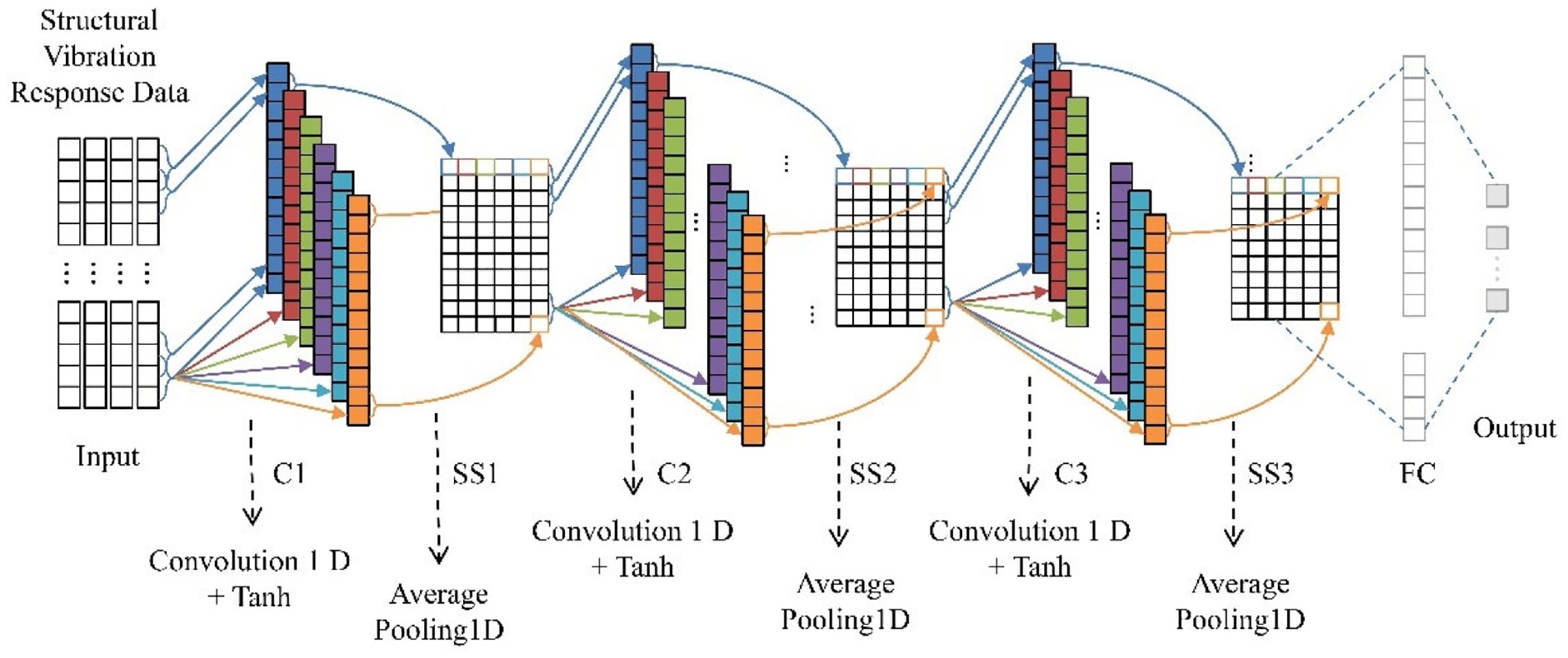
CNN framework.
For the input layer, structural dynamic acceleration responses are collected from a sensor network on the structure and numerical simulation from tests. A sample consists of collected acceleration time histories, which can be seen as feature types. Layers C1, C2, and C3, with 6, 12, and 12 filters, respectively, perform one-dimensional convolution, 27 followed by mean pooling layers SS1, SS2, and SS3. Mean pooling can retain the information of all the features. Mean pooling (Figure 2) takes the average value of each pooling window. The sizes of the C1, C2, and C3 filters and SS1, SS2, and SS3 pooling kernels depend on the size of input sample. The activation function is between the convolution and mean pooling layers, using the Tanh function, 28
where x is the input.
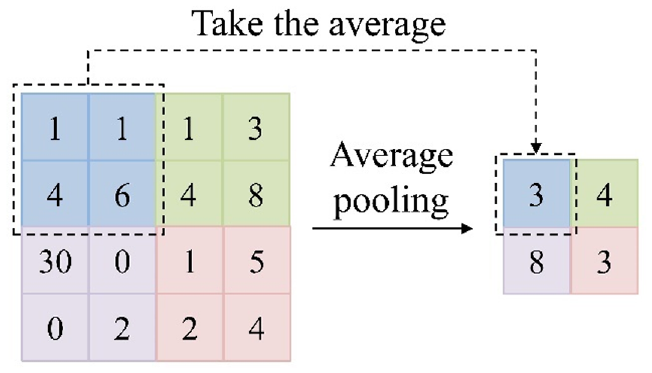
Average pooling.
SS3 is followed by a fully connected layer whose each neuron is connected with all the neurons in the previous layer, and whose local class distinction information it can integrate. At the end is an output layer, whose number of neurons is the number of the classes. Classification is made using a softmax function,
where Si is the probability that the current input sample is of the ith category, e is Euler’s number, Vi is the ith neuron of the output, and C is the number of categories.
The optimization algorithm adopts mini-batch gradient descent, and the loss function adopts a cross-entropy cost function,
where E is the loss, N is the total number of samples, y(i) is the ground-truth (label) of the ith sample, and o(i) is the output value of the ith sample.
DTL strategies
TL is a deep learning technology that can solve small data problems and enhance the robustness of neural networks. 29 DTL can be categorized as instance-based, mapping-based, network-based, or adversarial-based, 21 where network-based is most widely used, and is adopted for this work. A CNN is pretrained using samples of the source domain. Then, some layers of the CNN model are frozen. The parameters (weights and biases) of these layers are set as non-trainable. The network is retrained using samples of the target domain. Parameters (weights and biases) of frozen layers are not updated during training, so as to retain useful features learned in pretraining and reuse the target domain. DTL makes the training process more efficient because only parameters corresponding to unfrozen layers are updated. It can avoid overfitting of a network during the training process using small samples.
Layers are transferred, case by case, in network-based TL. In speech recognition, the model works better when the first few layers are trainable, and in image processing when the last few layers are trainable. 30 The first layers of CNN models extract features, and the last layers perform more abstract operations. We consider three representative DTL cases for defect identification in prefabricated structures, as shown in Figure 3. Figure 3(a) shows a pretrained deep CNN. In TL case 1 (Figure 3(b)), five middle layers of the CNN and their parameters (weights and biases) are frozen, and only the first convolutional layer, the fully connected layers, and the softmax layer are trainable. In TL case 2 (Figure 3(c)), the first four layers of the CNN and their parameters (weights and biases) are frozen, and the last convolutional layer, the last pooling layer, the fully connected layers, and the softmax layer are trainable. In fact, whether or not the pooling layer is frozen does not affect TL because mean pooling only takes the average value of each pooling window of the feature map extracted by the convolutional layer. In TL case 3 (Figure 3(d)), the first six layers of the CNN and their parameters (weights and biases) are frozen, and the fully connected layers and the softmax layer are trainable.
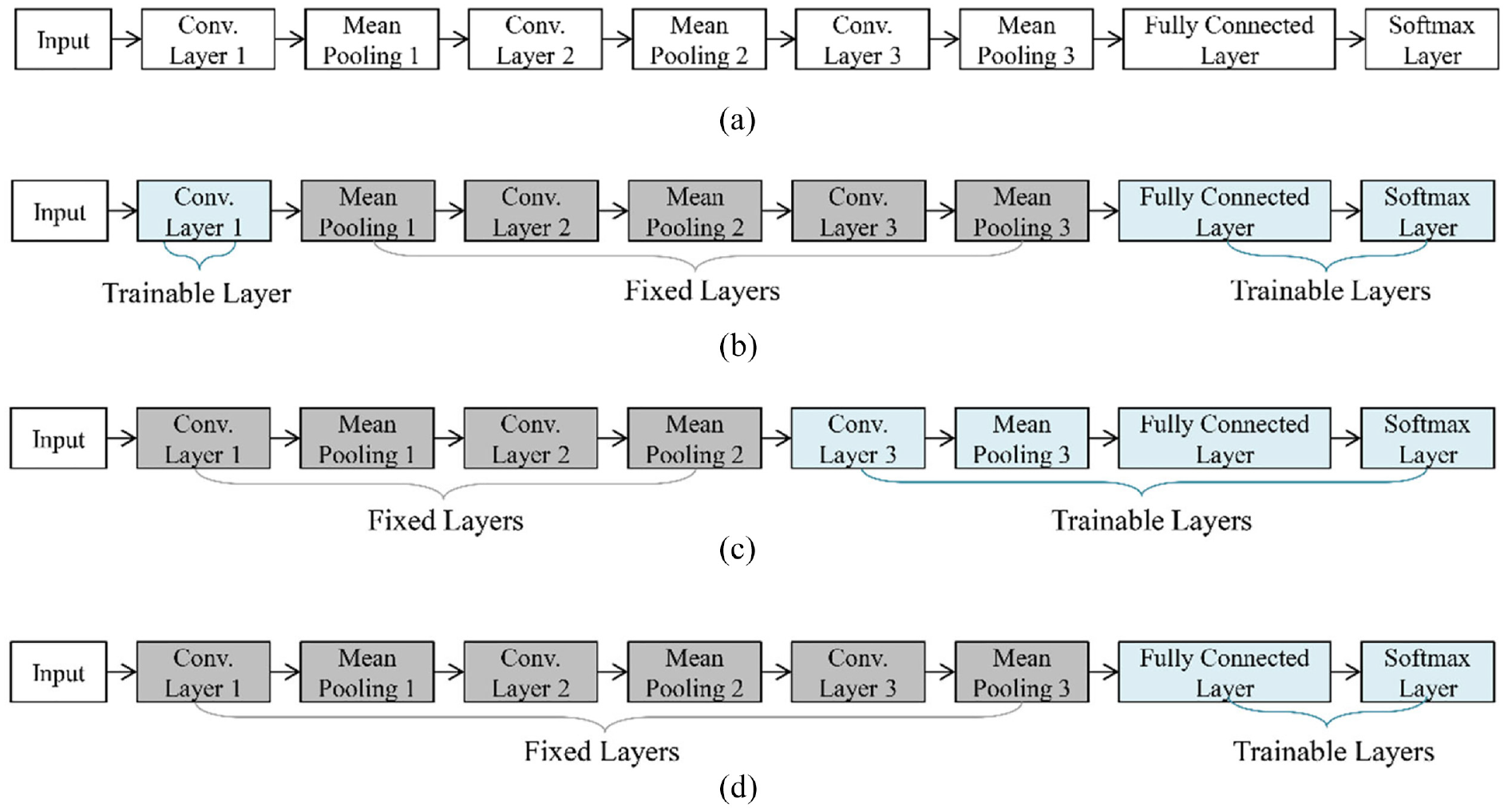
DTL cases: (a) pretrained CNN using samples from source domain; (b)TL case 1; (c) TL case 2; (d) TL case 3.
Experimental case study
Two full-scale prefabricated concrete shear wall structures with different defects were constructed to verify the performance of the proposed method.
Tests setup
Full-scale prefabricated concrete shear wall
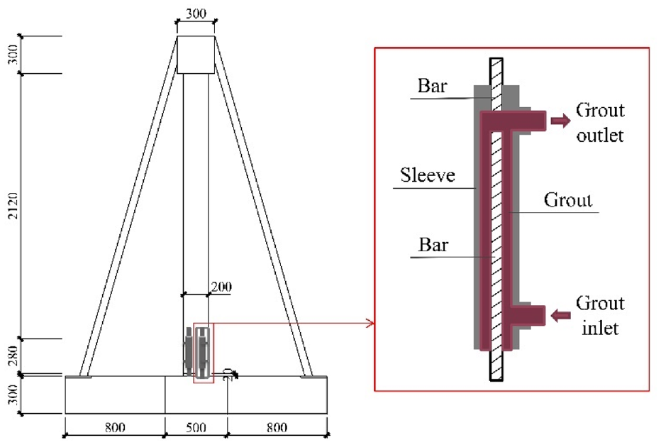
A full-scale prefabricated concrete shear wall structure was comprised of a top beam, a wall, and a ground beam, with elevation and top view as shown in Figure 4. As shown in Figure 5, an out-of-plane diagonal brace was set, connecting the top and ground beams, to impose constraints on the top beam. The upper end of the actual shear wall had a fixed boundary. Pre-embedded steel plates were embedded in the top and ground beams. The diagonal braces were welded to the embedded parts.
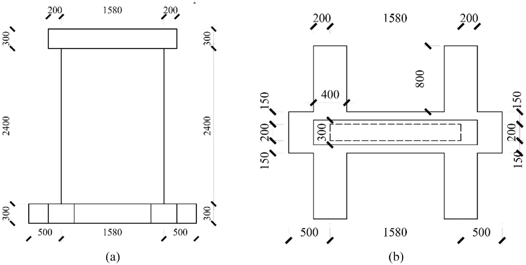
Elevation and top view of shear wall model: (a) elevation view and (b) top view.
Lateral view of shear wall model.
C30 concrete was used for beams and columns, and HRB400 steel bars for longitudinal reinforcements and stirrups. As shown in Figure 6, a full grouting sleeve connection method was adopted to connect the internal reinforcements at the connection between the shear wall and the foundation beam. The sleeve was nodular cast iron. The diameter of ribbed bars at the connection was 14 mm; the outer and inner diameters of the sleeve were 46 mm and 34 mm, respectively; and the length was 280 mm. 31 The shear wall and foundation beam components were prefabricated and assembled after curing in the laboratory of Tongji University. The Integral Concrete Technology was used for the top beam and wall. Figures 6 and 7, respectively, show the poured wall and ground beam before and after being spliced.
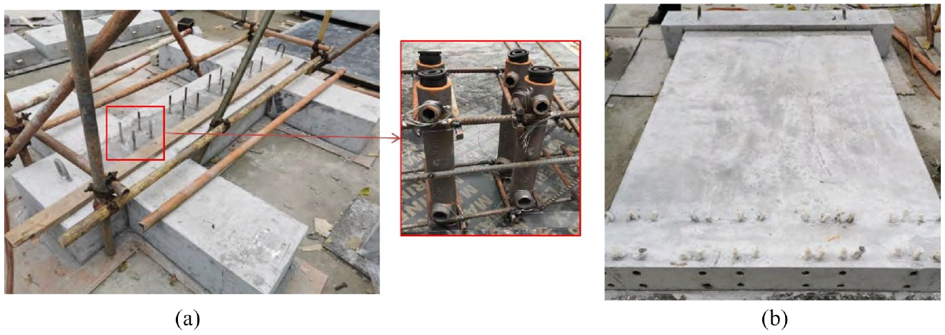
Physical diagrams of precast ground beam and poured wall: (a) ground beam and (b) poured wall.
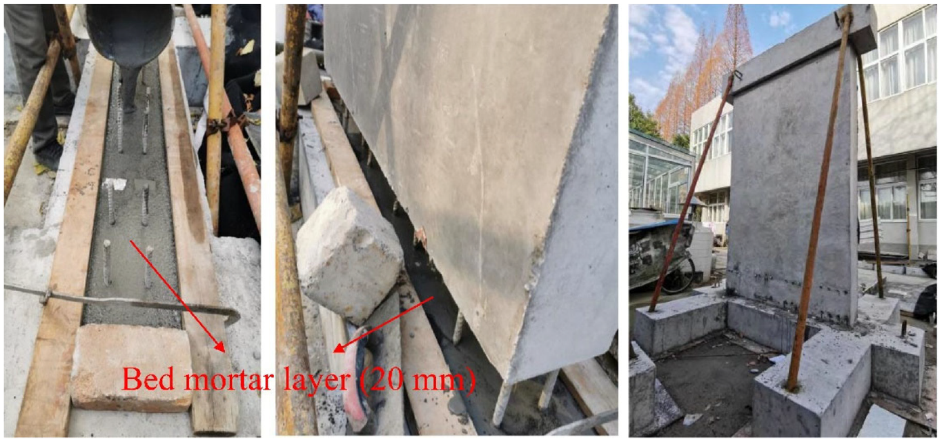
Physical diagram of prefabricated shear wall.
Defect settings
The two specimens were W1, which was the control group without defects, and W2, with incomplete fill of grout sleeve defects. As shown in Figure 8, from left to right, the prefabricated shear walls consisted of strips 1–4. The boundary conditions of side strips (1, 4) and middle strips (2, 3) can be considered as different. Figure 9 shows strips 1–4, which, respectively, have 3, 1, 2, and 4 incomplete fills of grout sleeves, with excitation points arranged in the center of each strip.
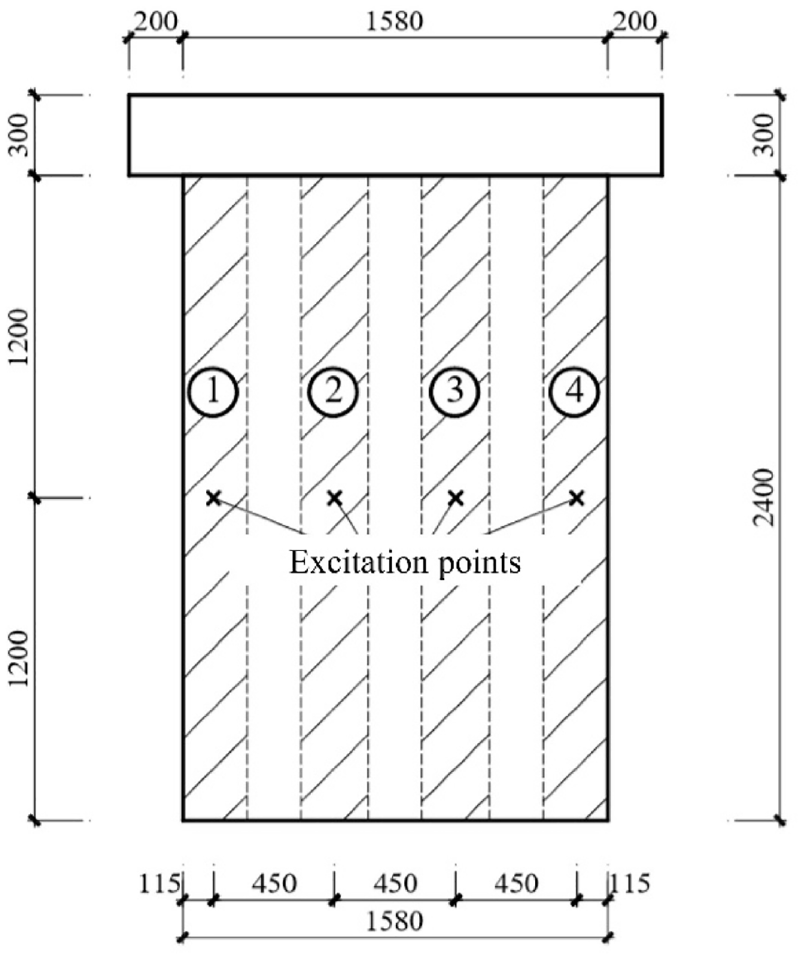
Strip division and excitation point arrangement.

Defect arrangement.
Dynamic excitation tests were carried out on the specimens W1 and W2. Then holes were drilled in the mortar layers of specimen W2 below the incompletely filled sleeves, and holes were drilled at the same location of Specimen W1. Dynamic excitation tests were carried out again on W1 and W2. Defect types were intact (type 1), incomplete fill of grout sleeve (type 2), through hole (type 3), and mix (type 4, combining types 2 and 3), as shown in Figure 10.
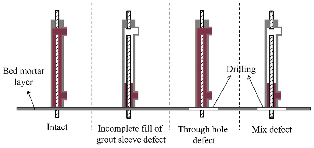
Defect types.
Excitation and measuring point arrangement
The excitation source for impact was a stainless-steel drilled pendulum with diameter 60 mm, aperture 5 mm, and weight 870 g. As shown in Figure 11, the vertical height of the pendulum suspension point and excitation point (pendulum impact point) was 500 mm. The pendulum ball was pulled to a predetermined height and released from a static state. It fell freely and hit the wall, forming an excitation vibration. To avoid errors due to different impact angles and uneven force, the same specifications of pads were pasted at the excitation point.
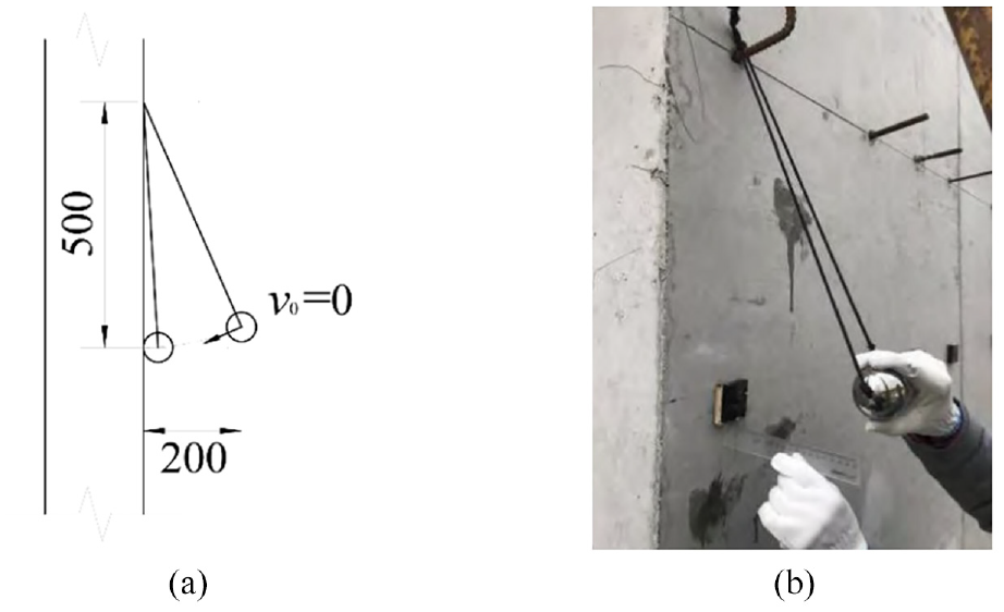
Excitation mode: (a) schematic diagram and(b) physical diagram.
Figure 12 shows the pendulum suspension, excitation, and measuring points. Acceleration sensors were arranged every 300 mm upward on each strip, starting from the upper surface of the bed mortar layer. Excitation was applied to the four strips of the W1 and W2 specimens in sequence, for a total of 16 working conditions. The acceleration responses of each measuring point were recorded and analyzed by self-spectrum. The acquisition frequency was 1024 Hz.
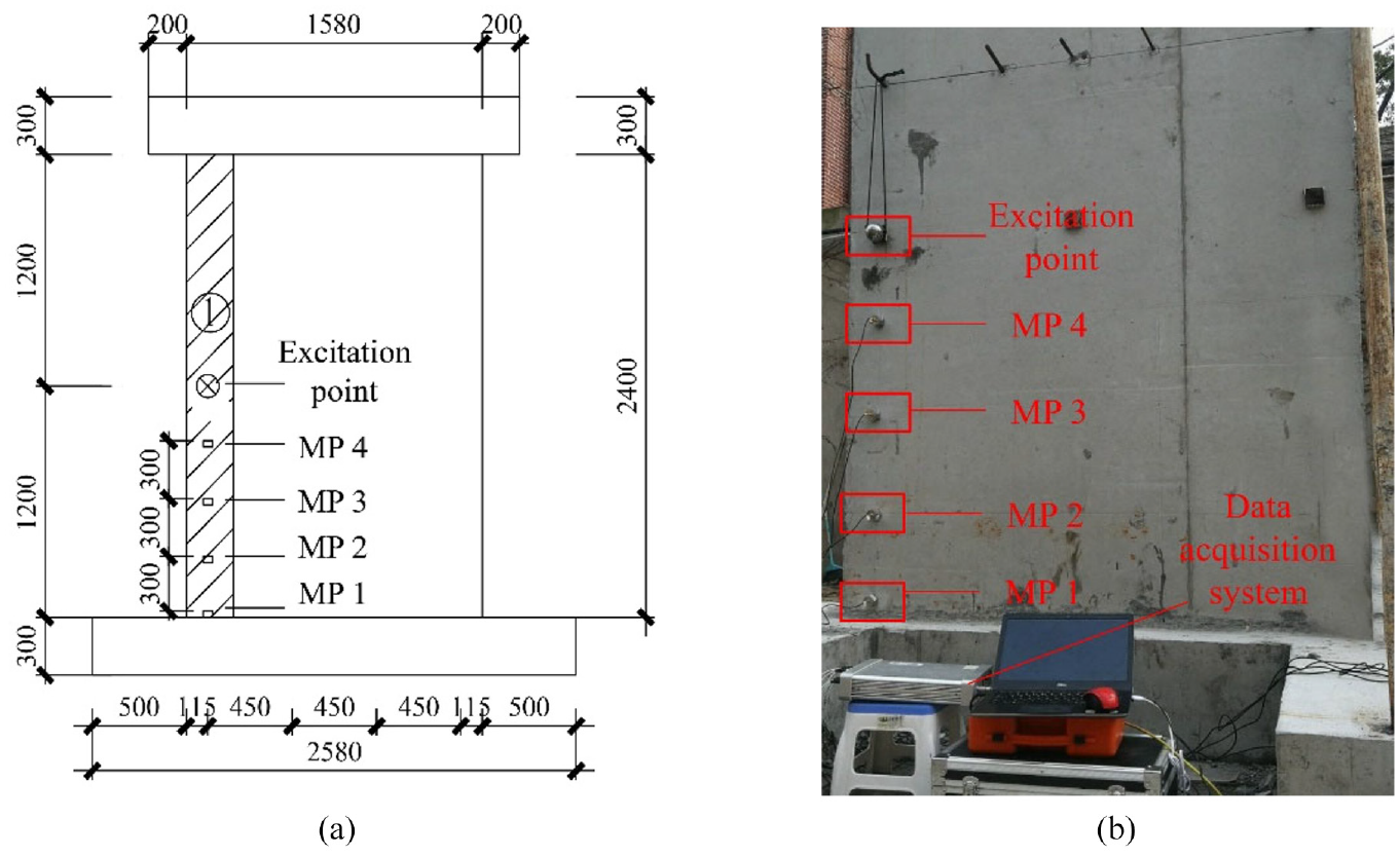
Layout of excitation point and measuring points of shear wall strip 1: (a) schematic diagram and (b) physical diagram.
Data collection and preprocessing
Excitation of duration 4 s was applied 50 times at the excitation point in each working condition, and acceleration responses were collected for each working condition. Each response set contained four acceleration time histories, each with 4096 signals. A 1-s segment (1024 signals) from each time history was subsequently analyzed. Data were normalized by min-max. 32 Data augmentation (multi-sample fusion, adding noise) was used to increase the data volume and diversity, which can enhance the generalization ability of CNN models. Samples were expanded to obtain more data. 33 Artificial data were created based on the real dataset. Figure 13 shows the procedure of multi-sample fusion data augmentation, which was as follows:
Four groups were randomly selected from the original acceleration time history samples, each containing acceleration time histories of four measuring points.
Acceleration time histories corresponding to four measurement points were randomly selected to form a new group.
Samples of each working condition were expanded from 50 to 1000. Dataset for each shear wall strip contains 4000 samples, of which the number of no defects, incomplete fill of grout sleeve defects, through hole defects, and mixed defects is 1000, respectively.
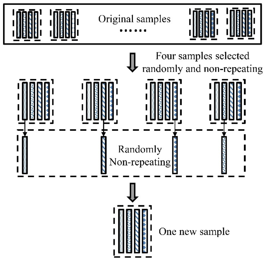
Data augmentation process.
Numerical simulation to enhance data diversity
Finite element model
A full-scale concrete prefabricated shear wall model, the same as the shear wall in the tests, was built using ABAQUS. As shown in Figure 14, its lower boundary condition was a fixed constraint, and the top beam was connected to the ground beam by double springs. At the connection of the wall and ground beam, 24 grouting sleeve connections were arranged to splice the steel bars. The material properties are shown in Table 1. The modal damping ratio of the concrete structure was 0.05. A C3D8R element was used to model the shear wall, and a T3D2 element to model the steel bar. As in the tests, the shear wall model was divided into four strips, with one excitation point and four measuring points arranged on each strip.
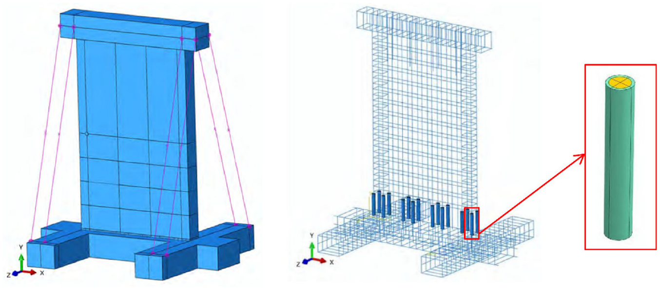
Finite element model.
Material parameters.

A shear wall strip was subjected to instantaneous impact excitation. A sine half-wave was used to simulate instantaneous impact excitation. 34 As shown in Figure 15, the duration of the excitation was 4 ms, with a peak excitation force of 1 kN. The acquisition frequency was 1024 Hz, and 150 acceleration signals were collected.
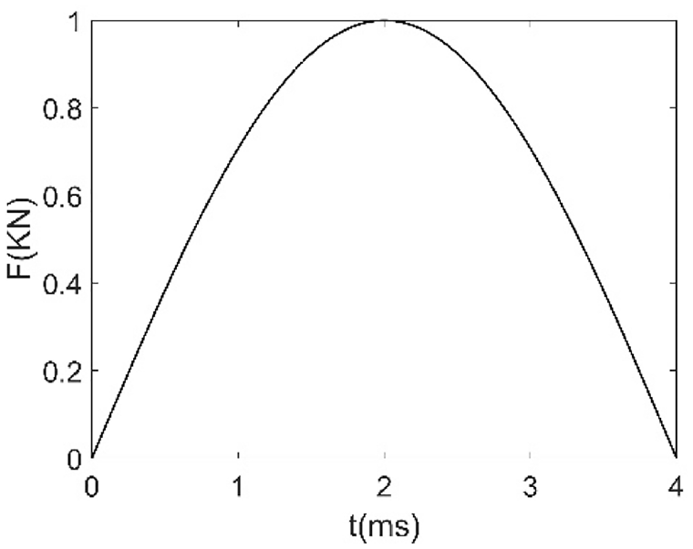
Sine half-wave excitation.
Defect setting
Shear wall strips were divided into side strips (1, 4) and middle strips (2, 3), with strips 1 and 2 taken as the research object. The incomplete fill of grout sleeve defect was introduced by reducing the elastic modulus of the grout to 3 N/m2. Each strip had defect degrees of 25%, 50%, 75%, and 100%. A strip was excited at the excitation point, and acceleration response data from four measuring points were collected. The acquisition frequency was 1024 Hz, and 150 signals were collected. Signals collected from four measuring points of one shear wall strip constituted a sample. The number of samples of each defect degree was expanded to 1000 by adding Gaussian random white noise. The signal-to-noise ratios corresponding to measuring points (MP1, MP2, MP3, and MP4) were randomly selected from the respective ranges of (55,65], (25,35], (15,25], and (15,25].
Defect identification on prefabricated concrete shear wall structures
Defect type identification
Sensing acceleration signals collected in tests were used to identify defect types. Each collected acceleration time history contained 1024 signals. Table 2 shows the CNN model configurations. There were 4000 samples of each shear wall strip, with equal proportions of each defect type, with 60% of the samples randomly selected for training, 20% for validation, and 20% for testing. The batch size was set to 5, and there were 50 epochs, so as to ensure sufficient samples for training. The learning rate was set to 0.01. Samples were labeled using one-hot encoding. One label vector had four elements, representing types 1–4. For example, the label vector [1, 0, 0, 0] represents the type of no defect.
CNN model configuration for defect type identification.
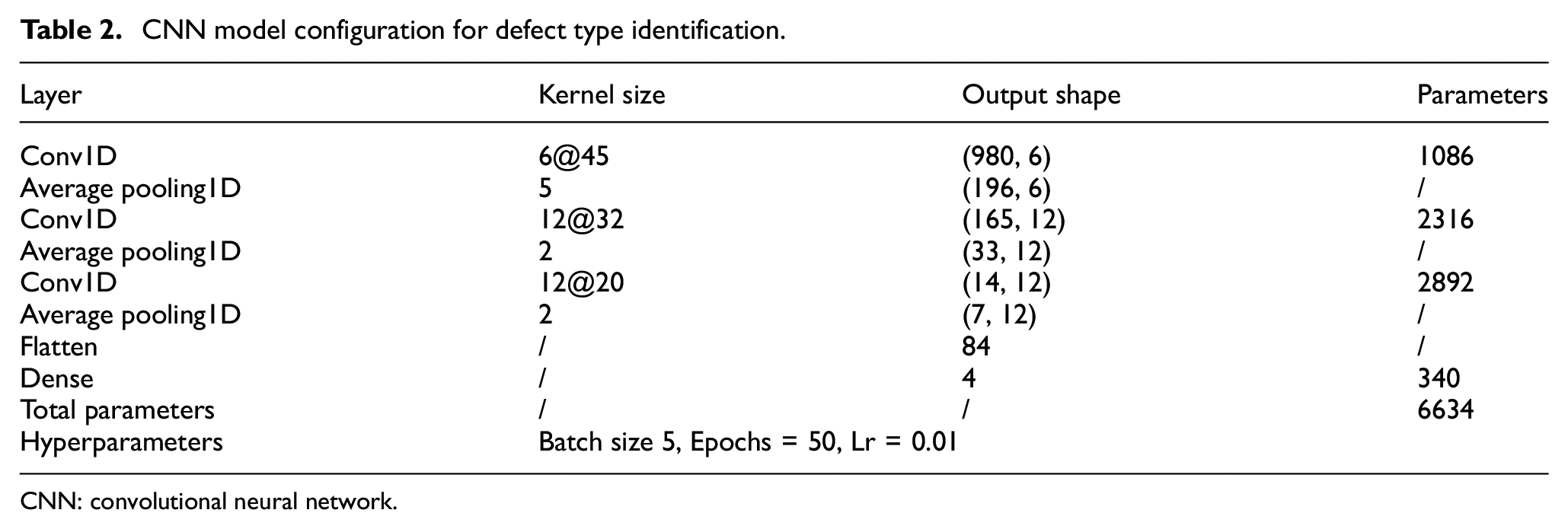
CNN: convolutional neural network.
Training CNNs for defect type identification using sufficient training samples
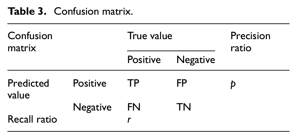
A CNN was trained using 2400 samples for defect type identification of shear wall strip 1, as shown in Figure 16. Figure 17 shows test results in the form of a confusion matrix, 34 with precision ratio (p) and recall ratio (r)
where TP is the number of samples whose true and predicted values are both positive, FP is the number of samples with a negative true value and positive predicted value, FN is the number of samples with a positive true value and negative predicted value, and TN is the number of samples whose true and predicted values are both negative, as shown in Table 3.
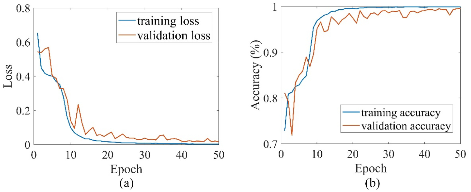
Training process (strip 1): (a) loss of training and validation set and (b) accuracy of training and validation set.
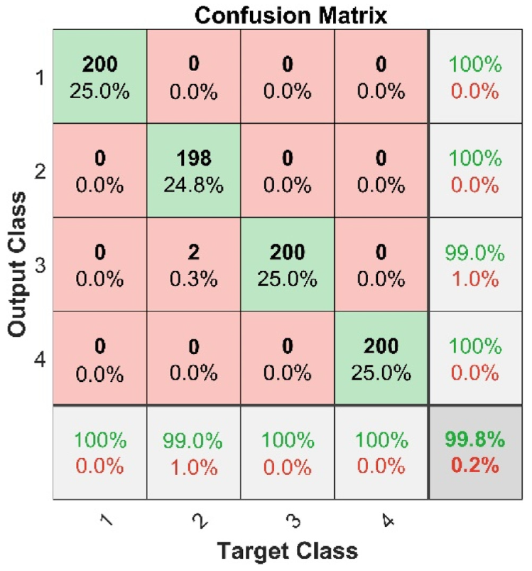
Confusion matrix (strip 1).
Confusion matrix.
As shown in Figure 16, there was no overfitting during training. 28 According to Figure 17, a CNN trained with sufficient training samples from the source domain can accurately identify defect types.
CNNs corresponding to shear wall strips 2, 3, and 4 were similarly trained. Their training loss, validation loss, training accuracy, and validation accuracy were monitored in real time to avoid overfitting. Figures 18–20 show their test results.
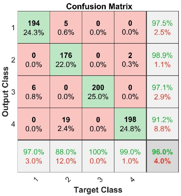
Confusion matrix (TL, strip 2).
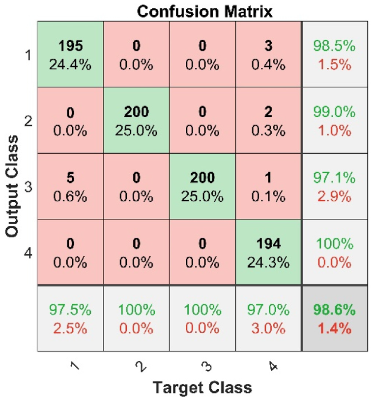
Confusion matrix (TL, strip 3).
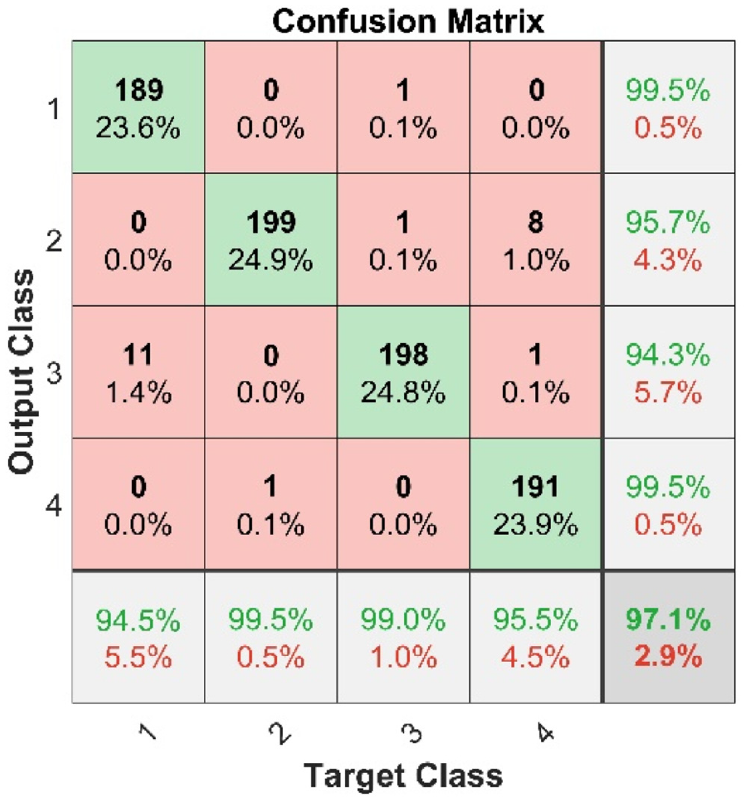
Confusion matrix (TL, strip 4).
Figures 18–20 show the identification results of the three CNNs trained on shear wall strips 2, 3, and 4, with almost all precision and recall ratios exceeding 95%. It can be concluded that CNNs trained with sufficient samples can accurately identify defect types. Incorrect classification mostly occurred between types 1 and 3 and between types 2 and 4. Hence, the impact of through hole defects in the bed mortar layer on the structural acceleration response was less than that of incomplete fill of grout sleeve defects. The trained CNN could perfectly identify incomplete fill of grout sleeve defects and through hole defects in the bed mortar layer with accuracy greater than 90%.
TL with CNN for defect type identification using small numbers of training samples
Shear wall strip 1 was taken as the source domain, and shear wall strips 2–4 as target domains. These domains differed by their boundary conditions and defects. Based on the pretrained CNN model corresponding to strip 1 (source domain), the CNN was retrained through the proposed DTL technology. To compare TL cases, the numbers of training, validation, and test samples were set to 800, 200, and 800, respectively. To verify and compare the performance of the proposed method on different levels of data scarcity, 400 training samples were used in TL case 3.
DTL from strip 1 to strip 2
The training processes are shown in Figures 21–24, and test results in Figures 25–28.
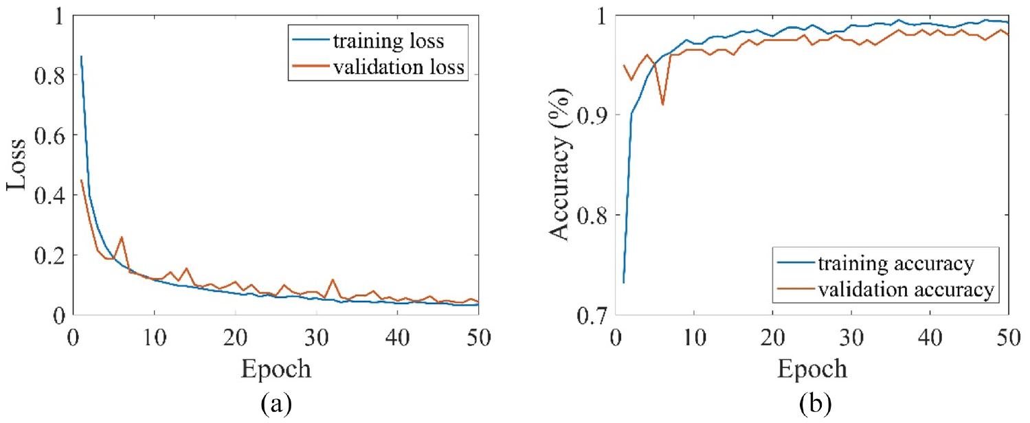
Training process (strip 2, TL case 1): (a) loss of training and validation set and (b) accuracy of training and validation set.
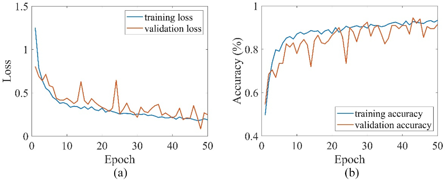
Training process (strip 2, TL case 2). (a) loss of training and validation set and (b) accuracy of training and validation set.
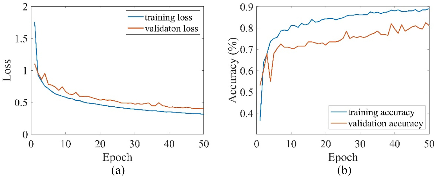
Training process (strip 2, TL case 3). (a) loss of training and validation set and (b) accuracy of training and validation set.
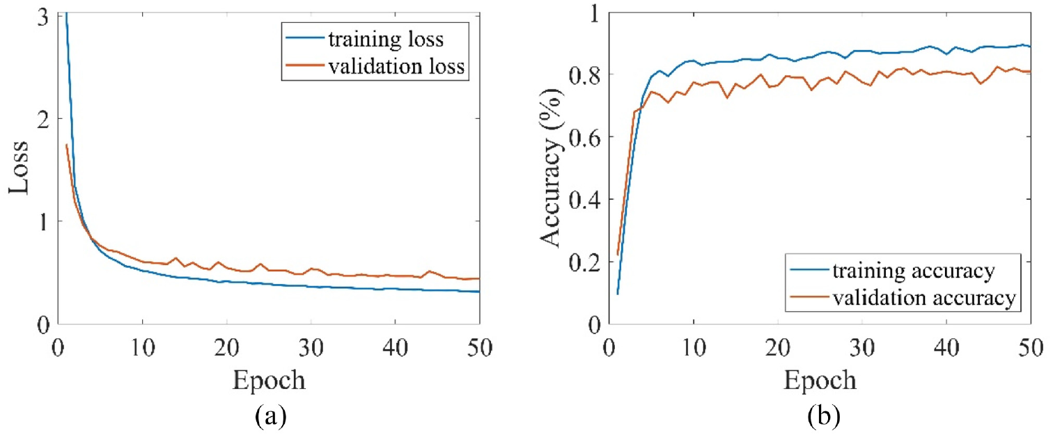
Training process (strip 2, TL case 3, 400 training samples). (a) loss of training and validation set and (b) accuracy of training and validation set.
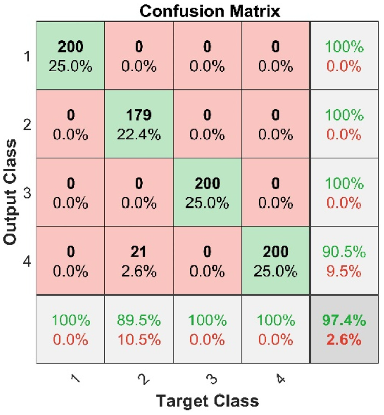
Confusion matrix (strip 2, TL case 1).
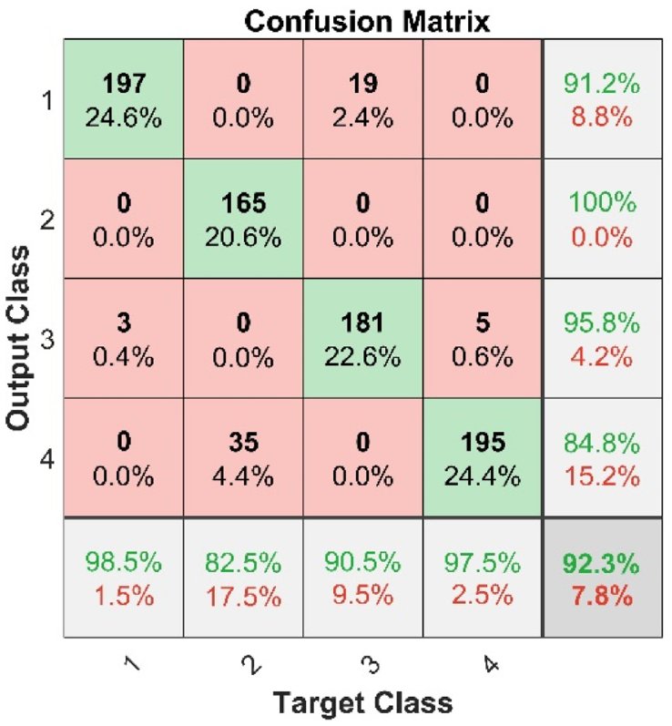
Confusion matrix (strip 2, TL case 2).
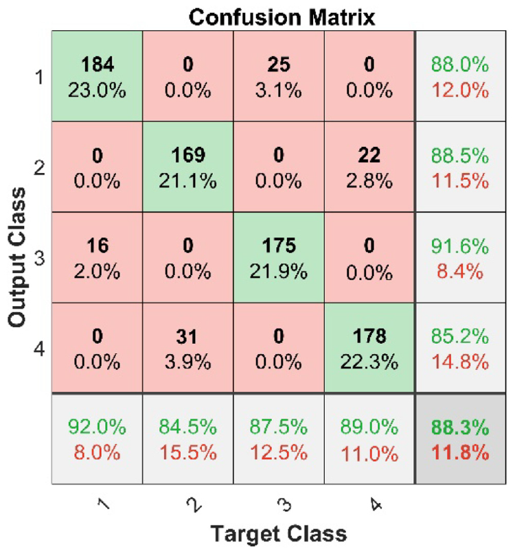
Confusion matrix (strip 2, TL case 3).
Confusion matrix (strip 2, TL case 3, 400 training samples).
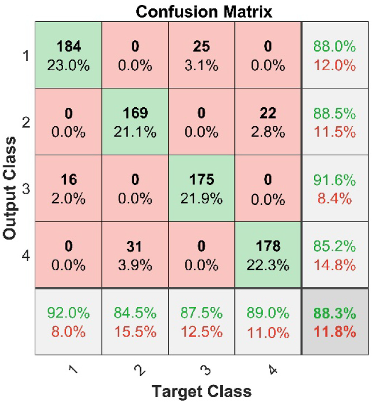
As shown in Figures 25–28, the CNN retrained using a small number of training samples from the target domain (shear wall strip 2) performed well at identifying defect types of shear wall strip 2. The identification accuracy of TL case 1 was higher than that of case 2, which was higher than that of case 3. It shows that the CNN models of TL case 1 and case 2 with one more trainable convolutional layer outperform that of TL case 3. In TL case 3, only fully connected layers and output layers of the CNN model are trainable. Case 1, with a trainable first convolutional layer, performed better than case 2, with a trainable last convolutional layer. Cases 1 and 2, with 800 training samples, had somewhat better identification accuracies than cases with 2400 training samples, because they utilized data from both the source and target domains. The identification accuracy of case 3, with just 400 training samples, was slightly less, but still high, at over 80%.
DTL from strip 1 to strip 3
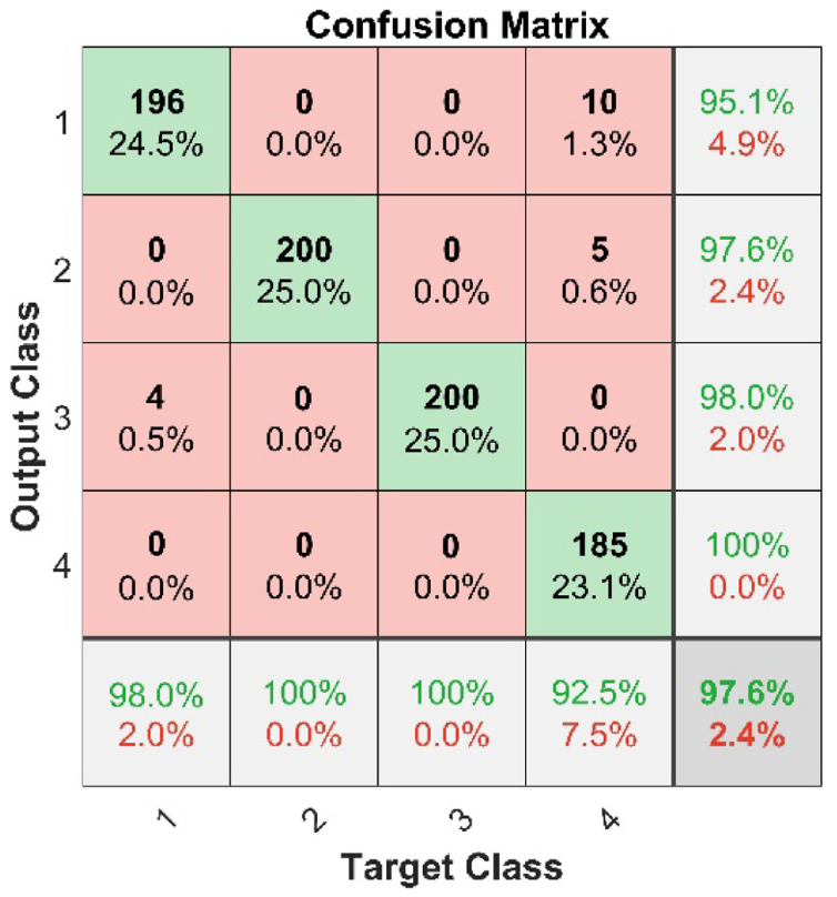
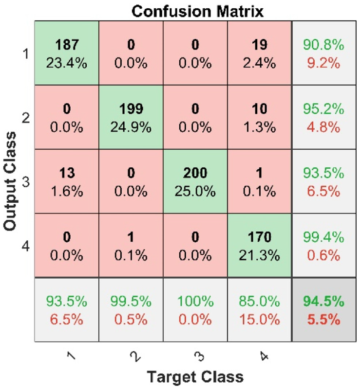
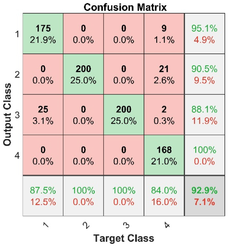
Test results are shown in Figures 29–32.
Confusion matrix (strip 3, TL case 1).
Confusion matrix (strip 3, TL case 2).
Confusion matrix (strip 3, TL case 3).
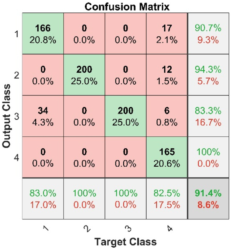
Confusion matrix (strip 3, TL case 3, 400 training samples).
The CNN retrained using a small number of training samples from the target domain (shear wall strip 3) performed well at the defect type identification of shear wall strip 3, with relative results similar to those of TL from strip 1 to strip 2.
DTL from strip 1 to strip 4
Test results are shown in Figures 33 and 34. The CNN retrained using a small number of training samples from the target domain (shear wall strip 4) performed perfectly at the defect type identification of shear wall strip 4, with 100% precision and recall ratios in TL cases 1–3. The results show that this method is more effective when the source and target domains have the same boundary conditions.
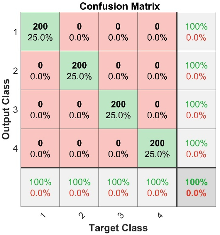
Confusion matrix (strip 4, TL case 1, 2, 3).
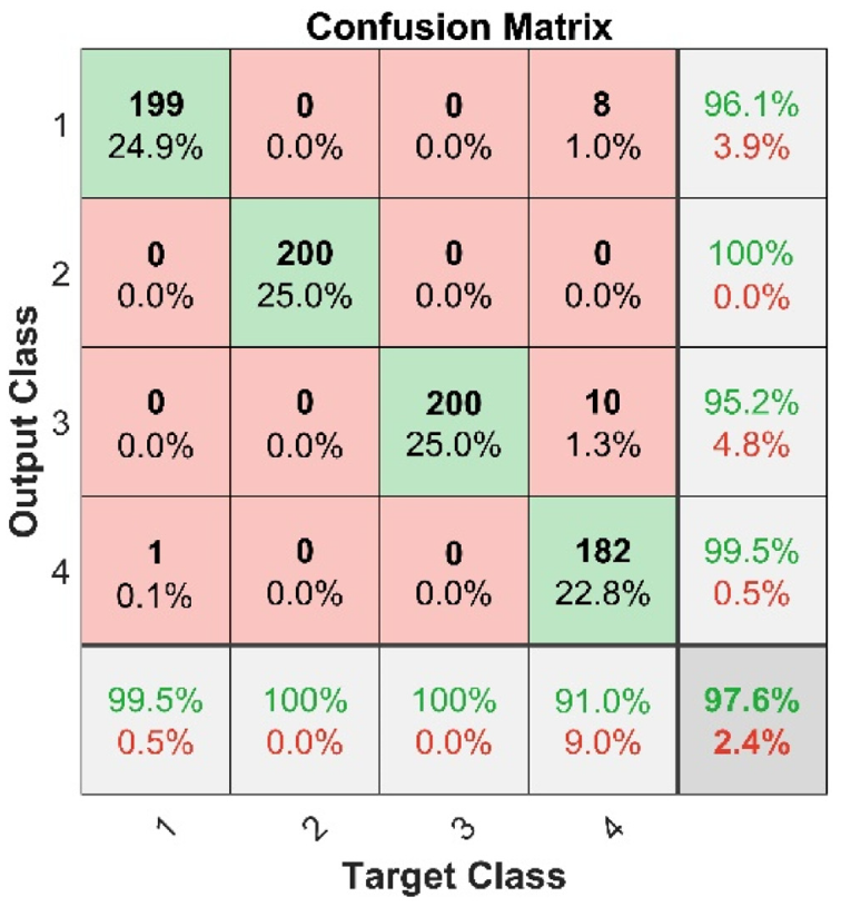
Confusion matrix (strip 4, TL 3, 400 training samples).
Defect degree identification
The defect degree of sensing acceleration signals collected in the tests of each shear wall strip was single. To verify the effectiveness of the proposed method in identifying defect degrees, these were supplemented with acceleration signals collected in numerical simulations. The acceleration time history collected from numerical simulations contained 150 signals. Fragments of the same length were intercepted from acceleration time history collected in the tests. Table 4 shows the configurations of the CNN models. There were four defect degrees (25%, 50%, 75%, and 100%). Shear wall strip 1 (side strip) and shear wall strip 2 (middle strip) were taken as the research objects for the identification of defect degrees, and their boundary conditions were different. The dataset of shear wall strip 1 contained 1000 sensing acceleration signal samples (incomplete fill of grout sleeve defects with degree 75%) collected in tests, and 3000 acceleration signal samples (defect degrees: 25%, 50%, and 100%) collected in numerical simulations. The dataset of shear wall strip 2 contained 1000 sensing acceleration signal samples (incomplete fill of grout sleeve defects with degree 25%) collected in tests and 3000 acceleration signal samples (defect degrees: 50%, 75%, and 100%) collected in numerical simulations. Samples (four defect degrees in equal proportions) were randomly selected, with 60% for training, 20% for validation, and 20% for testing. The batch size was 10, there were 300 epochs, and the learning rate was 0.01. Samples were labeled using one-hot encoding. One label vector consisted of four elements, representing 25%, 50%, 75%, and 100% defect degrees.
Configuration of CNN model for defect degree identification.
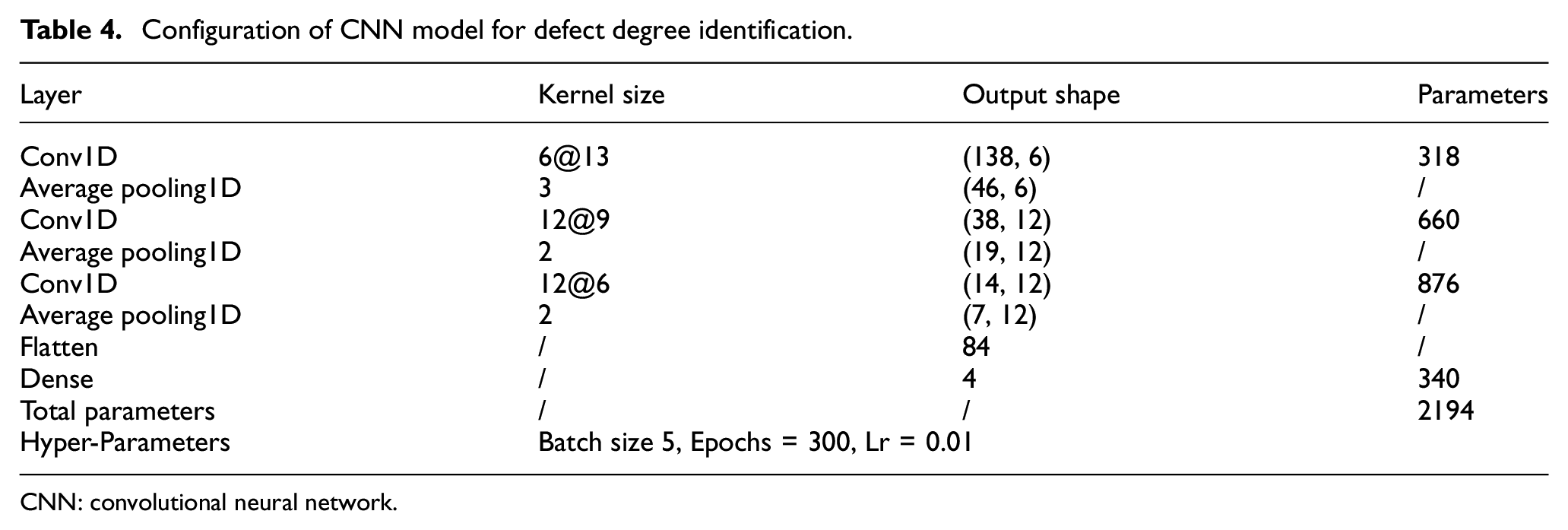
CNN: convolutional neural network.
Training CNNs for defect degree identification using sufficient training samples
For defect degree identification of shear wall strips 1 and 2, two CNNs were trained using 2400 training samples. The training process is shown in Figures 35 and 36, and test results in Figures 37 and 38.
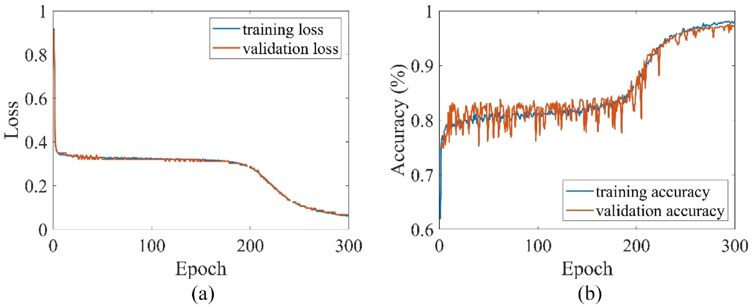
Training process (strip 1): (a) loss of training and validation set and (b) accuracy of training and validation set.
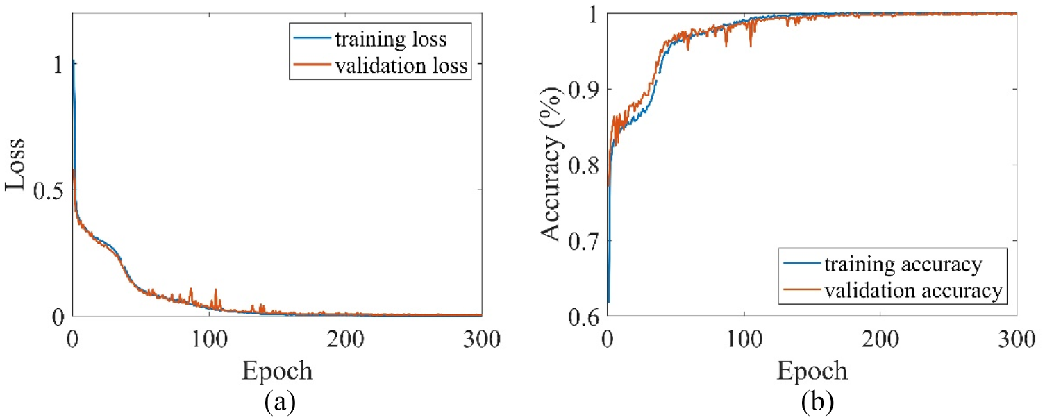
Training process (strip 2). (a) loss of training and validation set and (b) accuracy of training and validation set.
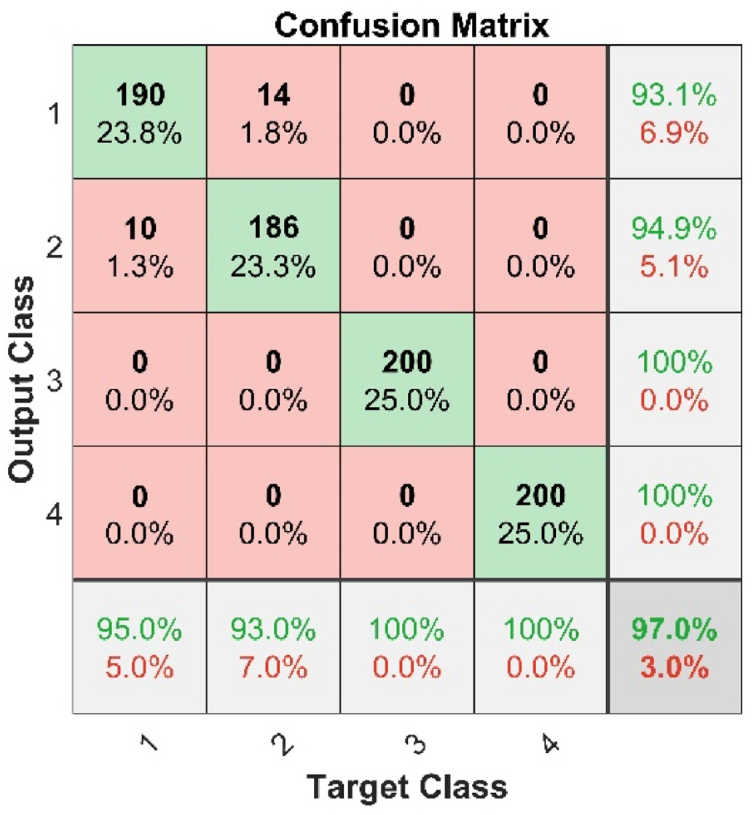
Defect degree identification confusion matrix(strip 1).
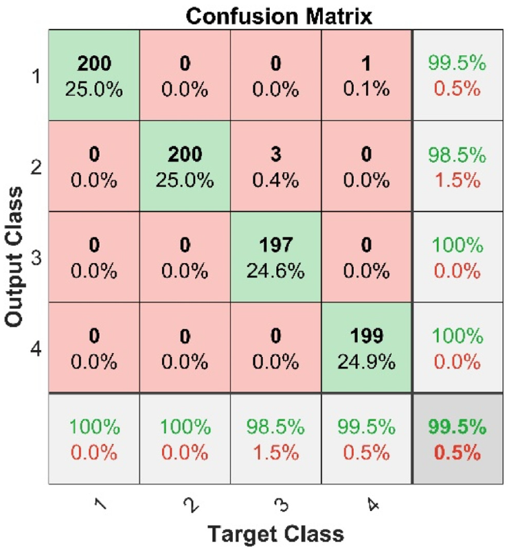
Defect degree identification confusion matrix(strip 2).
Results show that a CNN trained with sufficient training samples can identify defect degrees with high accuracy.
TL with CNN for defect degree identification using small numbers of training samples
Shear wall strip 1 was taken as the source domain, and shear wall strip 2 as the target domain. These domains differed due to their boundary conditions. Based on the pretrained CNN of strip 1 (source domain) for defect degree identification, the CNN was retrained through the proposed DTL technology on shear wall strip 2. To compare the performance of different cases, the numbers of training, validation, and test samples were set to 800, 200, and 800, respectively. For TL case 3, the pretrained CNN was retrained using 400 training samples.
The training processes were monitored for DTL from strip 1 to strip 2, with test results as shown in Figures 39–42.
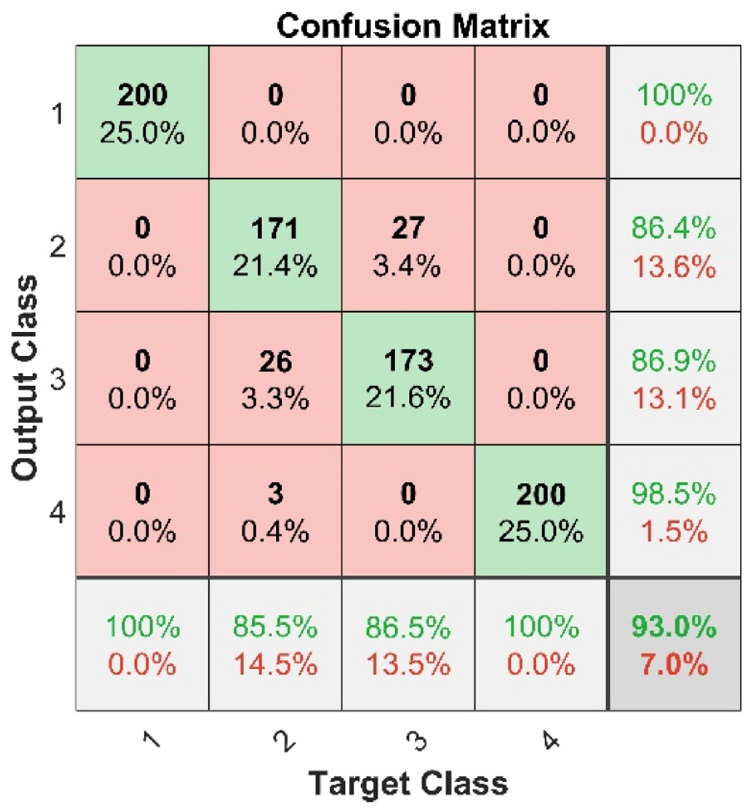
Defect degree identification confusion matrix(TL case 1).
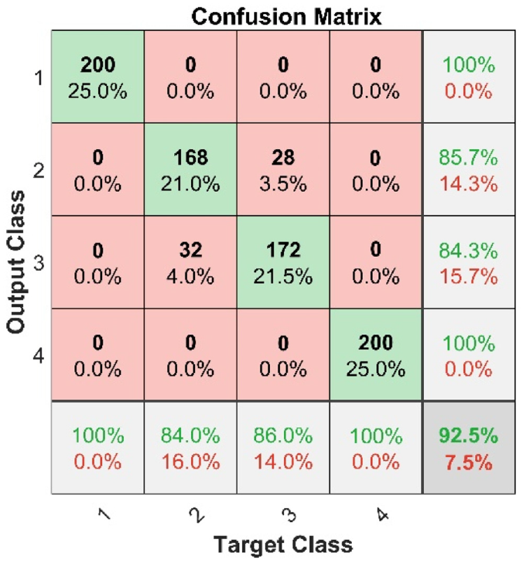
Defect degree identification confusion matrix(TL case 2).
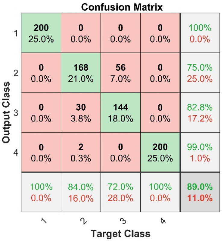
Defect degree identification confusion matrix(TL case 3).
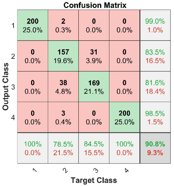
Defect degree identification confusion matrix(TL case 3, 400 training samples).
As shown in Figures 39–42, the CNN retrained using a small number of training samples from the target domain (shear wall strip 2) performed well in the defect degree identification of shear wall strip 2, which is similar to the TL from strip 1 to strip 2 in defect type identification.
Conclusion
We proposed a defect identification method with a basic neural network framework of a one-dimensional CNN and TL, and the method was verified on prefabricated concrete shear walls. Data were collected through non-destructive dynamic tests and corresponding numerical simulation, and different TL strategies were compared. Test results showed that the proposed method has excellent performance in defect identification in prefabricated concrete structures, and works with a small number of training samples. In this study, DTL models trained using a small number of samples outperformed traditional CNN models trained using sufficient samples. Compared to the DTL models with trainable fully connected layer and output layer, DTL models with trainable one convolutional layer, fully connected layer, and output layer had a better performance. And DTL models with a trainable first convolutional layer performed better than with a trainable last convolutional layer. By comparing the proposed method on different target domains, it can be concluded that it is more effective when the source and target domains have the same boundary conditions. The proposed method is more efficient than traditional CNN methods due to its lower training time.
Footnotes
Declaration of conflicting interests
The author(s) declared no potential conflicts of interest with respect to the research, authorship, and/or publication of this article.
Funding
The author(s) disclosed receipt of the following financial support for the research, authorship, and/or publication of this article: This research was supported by the Ministry of Science and Technology of the People’s Republic of China (Grant No. SLDRCE19-B-02), the Shanghai Municipal Science and Technology Major Project (2021SHZDZX0100), and the Fundamental Research Funds for the Central Universities.
