Robit regression in Stata

Abstract

Logistic and probit models are the most popular regression models for binary outcomes. A simple robust alternative is the robit model, which replaces the underlying normal distribution in the probit model with a Student’s t distribution. The heavier tails of the t distribution (compared with the normal distribution) mean that model outliers are less influential. Robit regression models can be fit as generalized linear models with the link function defined as the inverse cumulative t distribution function with a specified number of degrees of freedom; they have been advocated as being particularly suitable for estimating inverse-probability weights and propensity scoring more generally. Here we describe a new command, robit, that implements robit regression in Stata.

Keywords

st0724 robit xlink robit regression binary regression generalized linear models inverse-probability weights

1 Introduction

Robit regression models are similar to probit models, but the underlying normal distribution in the latter is replaced by a central Student’s t distribution with a zero median and ν degrees of freedom (d.f.). More formally, they can be defined as generalized linear models (GLMs) with a binomial family (usually Bernoulli) variance function and a robit link function with ν d.f.

The Student’s t distribution resembles a normal distribution in that it is symmetrical and bell shaped, but it has heavier tails. Thus, it has been advocated as an alternative to the normal distribution in defining regression models for continuous outcomes, without giving too much influence to outlying values. For example, this was done by Zellner (1976) and by Lange, Little, and Taylor (1989). These ideas were extended to regression models with binary outcomes (see, for example, Liu [2004]).

Compared with the better-known probit and logit link functions, the robit link gives less influence to observations that are highly unlikely given the values of the predictors. This property is discussed in Mudholkar and George (1978), Albert and Chib (1993), Liu (2004), and Kang and Schafer (2007) and is thought to make the robit link particularly suited for use in estimating probability weights.

Seaman and White (2013) recommended the use of robit models for computing inverse-probability weights to handle missing-at-random values, and they included this method in a list of useful techniques that are “not routinely available in most statistical software.” In the case of robit regression and Stata, this is no longer true. Here we present a command, robit, that enables robit regression in Stata.

2 Methods and formulas

Robit models are a special class of GLMs. GLMs were introduced by McCullagh and Nelder (1989) and are implemented in Stata using the glm command. Specifically, robit regression corresponds to a GLM with a binomial (usually Bernoulli) variance function and a robit link function.

In general, a link function η(µ) is an invertible monotonic transformation of the conditional mean µ, equal to a conditional probability in the case of a Bernoulli model. For instance, the logit link is defined as

η (μ) = ln {μ / (1 - μ)}

and the probit link is defined as

η (μ) = Φ^{- 1} (μ)

where Φ(·) is the cumulative standard normal distribution function and Φ ⁻ ¹(·) is its inverse. And both of these link functions have twice-differentiable inverses. To fit a GLM with a specified link function, we need to be able to generate variables containing the link function η(µ) from the conditional mean µ, the inverse link function µ(η) from the link function, and also the first two derivatives of µ with respect to η.

A robit link function (also known as a t-link function) with ν d.f. is defined by substituting an inverse cumulative t distribution function for the inverse cumulative standard normal distribution function in the probit link function, as

η (μ) = F_{t (ν)}^{- 1} (μ)

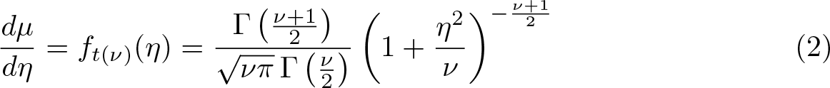
where F_t ₍ _ν ₎(·) is the cumulative Student’s t distribution function with ν d.f. and $F_{t (ν)}^{- 1}$ (·) is its inverse. This link function also has a twice-differential inverse, with a first derivative given by

\frac{d μ}{d η} = f_{t (ν)} (η) = \frac{Γ (\frac{ν + 1}{2})}{\sqrt{ν π} Γ (\frac{ν}{2})} {(1 + \frac{η^{2}}{ν})}^{- \frac{ν + 1}{2}}

where f_t ₍ _ν ₎(·) is the density function for the t distribution with ν d.f. Therefore, differentiating (2) with respect to η, defining u = 1 + η ²/ν, and using the chain rule, we have the second derivative of µ with respect to η as

\frac{d^{2} μ}{d η^{2}} = \frac{d}{d u} (\frac{d μ}{d η}) \frac{d u}{d η} = - \frac{Γ (\frac{ν + 1}{2})}{\sqrt{ν π} Γ (\frac{ν}{2})} \frac{2 η}{ν} \frac{ν + 1}{2} {(1 + \frac{η^{2}}{ν})}^{- \frac{ν + 3}{2}}

The formulas (1), (2), and (3) define the variables that we need to generate for glm to fit a robit model. Because the official glm command does not allow the specification of robit models, we wrote user-defined robit link functions to do this. See User-defined functions under Remarks and examples of [R] glm for technical details of how this is done.

Figure 1 shows the inverse robit link functions (also known as t distribution functions) with d.f. 1, 4, and 10, together with the inverse probit link function (also known as the normal distribution function or as a t distribution function with infinite d.f.). Note that the fewer d.f. there are, the further µ(η) is from 0 (in the case of negative η) or from 1 (in the case of positive η).

Figure 1.

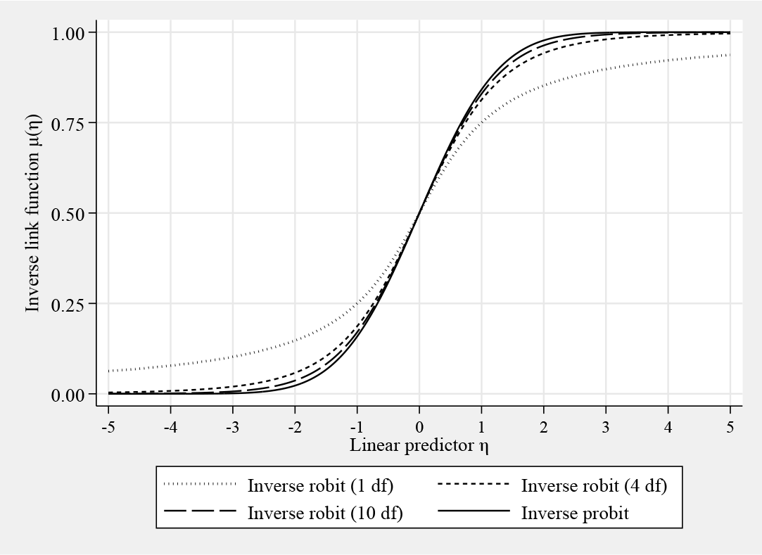
Inverse robit and probit link functions µ(η)

The choice of d.f. for robit models still seems to be an open question. Kang and Schafer (2007) recommended 4 d.f., and, commenting on this article, Ridgeway and McCaffrey (2007) discuss and demonstrate the possibility of 1 d.f. Liu (2004) described 7 d.f. as being an excellent approximation to the logit link function but less influenced by model outliers. Albert and Chib (1993) discussed the case of 8 d.f. Robit with 9 d.f. was mentioned by Mudholkar and George (1978) as having a similar kurtosis to the logit link function. In general, robit link functions with fewer d.f. are influenced less by outliers than those with more d.f. In the limit, as ν tends to infinity, the robit model with ν d.f. becomes the probit model. The d.f. of a robit model can be either prespecified by the user (for computational simplicity, as implemented in our robit command) or estimated together with the other parameters of the model, possibly using an expectation maximization-type algorithm as discussed in Liu (2006). Gelman, Hill, and Vehtari (2021), in their chapter 15, express the view that an estimate of the d.f. from the data “might be noisy.”

Note that the t distributions used by our packages are all standard t distributions, specified uniquely by their d.f. Chapter 15 of Gelman, Hill, and Vehtari (2021) discusses the possibility of defining robit link functions using generalized t distributions (with added scale parameters) to modify the units in which the parameters are expressed. Generalizations of the t distribution are reviewed, for example, in Li and Nadarajah (2020).

3 The robit command

3.1 Syntax

robit depvar [indepvars] [if] [in] [weight], dfreedom( # ) [noconstant offset( varname ) constraints( constraints ) asis vce( vcetype ) level( # ) noheader notable collinear coeflegend difficult from( init_specs )]

depvar is a dependent variable that must be binary.

fweights, aweights, iweights, and pweights are allowed; see [U] 11.1.6 weight.

robit has all the features available after estimation for glm, such as the predict and margins commands. See [R] glm postestimation.

3.2 Description

robit fits a robit regression model with a number of d.f. specified by the user. It requires the Statistical Software Components (SSC) package xlink (Newson 2021) to work.

3.3 Options

dfreedom( # ) specifies the d.f. for the robit model to be fit. It must be specified as an integer between 1 and 10. dfreedom() is required.

noconstant suppresses the constant term (intercept) in the model.

offset ( varname ) specifies that varname be included in the model as an offset with the coefficient constrained to be 1.

constraints ( constraints ) specifies the linear constraints to be applied during estimation. The default is to perform unconstrained estimation. See [R] Estimation options.

asis forces retention of perfect predictor variables and their associated, perfectly predicted observations. This may produce instabilities in maximization; see [R] probit.

vce( vcetype ) specifies the type of standard error (SE) reported. Possible types include those that are derived from asymptotic theory (oim, opg), those robust to some kinds of misspecification (robust), those that allow for intragroup correlation (cluster clustvar), and those from bootstrap or jackknife methods (bootstrap, jackknife); see [R] vce_option .

level( # ) specifies the confidence level. The default is level(95). See [R] Estimation options.

noheader suppresses the header information from the output. The coefficient table is still displayed.

notable suppresses the table of coefficients from the output. The header information is still displayed.

collinear specifies that the estimation command not omit collinear variables. This option is seldom used because collinear variables make a model unidentified. However, you can add constraints to a model that will identify it even with collinear variables. See [R] Estimation options for details.

coeflegend instructs Stata not to show the coefficient results but instead to display the legend of the coefficients and how they should be specified in an expression.

difficult specifies that the likelihood function is likely to be difficult to maximize because of nonconcave regions. There is no guarantee that difficult will work better than the default; sometimes it is better and sometimes it is worse. You should use the difficult option only when the default stepper declares convergence and the last iteration is “not concave” or when the default stepper is repeatedly issuing “not concave” messages and producing only tiny improvements in the log likelihood. See [R] Maximize.

from( init_specs ) specifies initial values for the regression coefficients. See [R] Maximize.

3.4 Remarks

robit works by calling glm with a user-defined robit link function and a Bernoulli distribution family. More in detail, the link function is specified as robit followed by an integer between 1 and 10 representing the d.f.; for example, link(robit7) corresponds to a robit link function with 7 d.f. We collected these community-contributed robit link functions into an SSC package called xlink, which must be installed for robit to work.

robit is designed to be user friendly and not to require advanced Stata or statistical skills. Users who want to fit robit models with the full power of glm can use glm directly with a robit function from xlink. For example, robit y x1 x2, dfreedom(4) is equivalent to glm y x1 x2, family(binomial) link(robit4). The use of glm in place of robit may be advantageous when, for instance, the specification of nonstandard maximization (see [R] Maximize) or display (see [R] Estimation options) options is needed.

3.5 Stored results

robit stores in e() all results stored by glm with a robit link and a Bernoulli variance family, and it also stores the following:

4 Examples

4.1 Creating an outlier in a simulated dataset

We illustrate the use of our robit command using a two-scenario simulation, similar in spirit to the one in chapter 15 of Gelman, Hill, and Vehtari (2021). We generated data for 200 subjects, aiming to estimate the effect of a predictor x on a binary outcome d (1 if a subject has a disease, 0 otherwise). We assumed the predictor to be normally distributed (as might be the case with the log of a biological assay result), with mean 0 and standard deviation 5. In the first scenario (the base scenario), we simulated a binary outcome d, using a logistic model with an intercept (log odds for zero x) of −3 and a log odds-ratio of 1 per unit of x. This was done using the code

(See Buis [2007] for more about simulating binary and other discrete models.) In the second scenario (the outlier scenario), we introduced an outlier by switching the outcome of an extreme x value from 0 to 1. Specifically, we created a new binary variable, d2, that was like d in the first scenario, except that the subject with the smallest x value (and therefore with the lowest probability of disease in the base scenario) was diagnosed (or misdiagnosed) as having the disease. Note that outliers are usually thought of as extreme observations but, in the context of binary outcomes, are usually observations that are highly unlikely given the values of the predictors.

Of the 200 subjects, 52 had the disease in the base scenario, increasing to 53 in the outlier scenario (because the outcome of one observation was switched from 0 to 1). We fit 3 binary regression models:

a logit model for the base scenario, regressing d with respect to x;

a logit model for the outlier scenario, regressing d2 with respect to x; and

a robit model with 4 d.f. for the outlier scenario, regressing d2 with respect to x.

We used Huber (or “robust”) variances for consistency throughout because not all the models were correctly specified, although we knew that the first one was, having carried out the simulation under it. For each of the three models, we estimated the probability of having the disease as a function of x. Note that using Huber variances does not affect the point estimates or the predicted probabilities.

The logit model for the base scenario gave the following results:

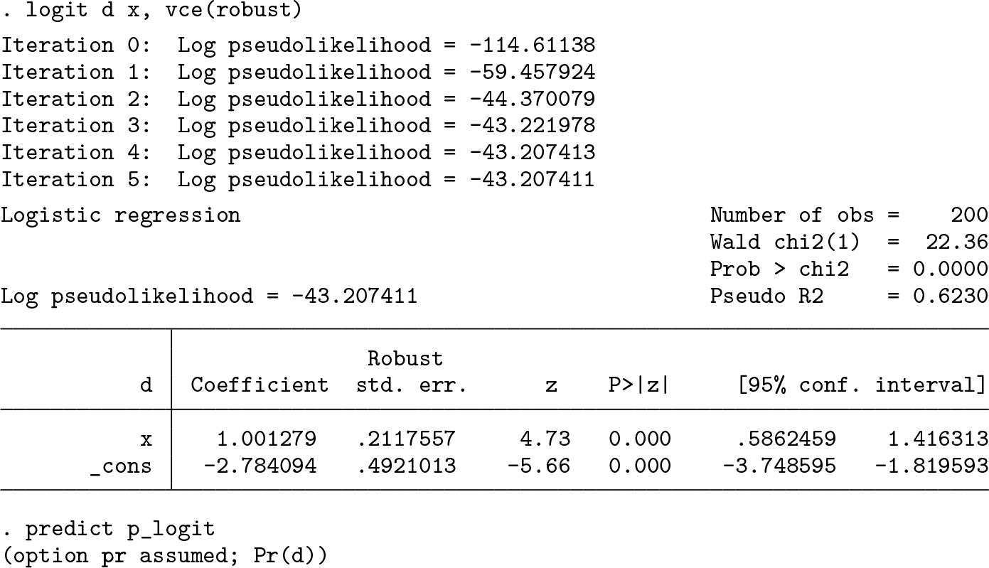
We see that the estimated log odds-ratio is 1.001 per unit of x (95% confidence interval [CI] [0.586 to 1.416]).

The logit regression in the outlier scenario produced the following output:

This time, the log odds-ratio per x unit is estimated as 0.710 (95% CI [0.286 to 1.135]). Therefore, creating the outlier has reduced the estimated log odds-ratio (nonsignificantly).

The robit model under the outlier scenario produced output as follows:

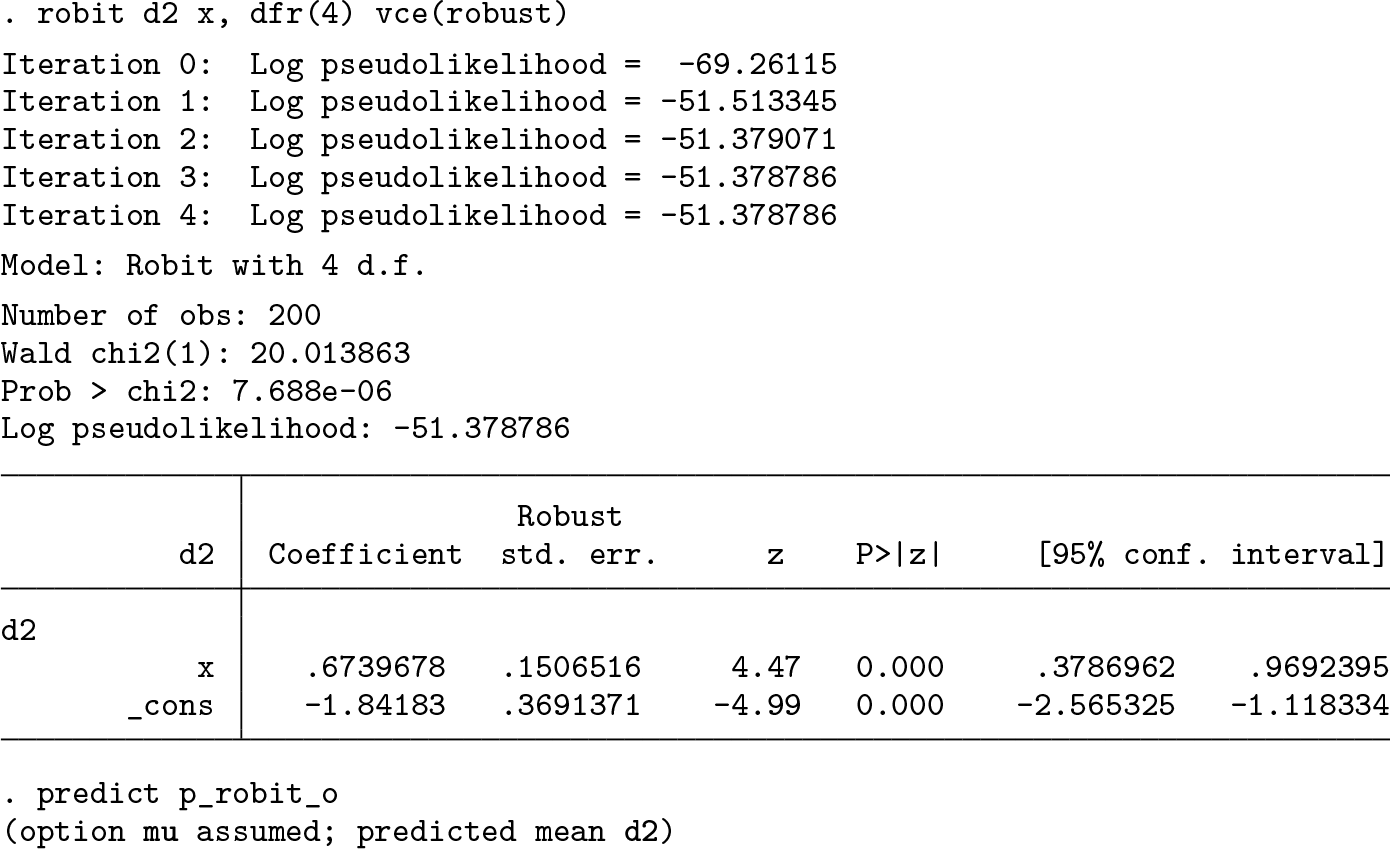
This time, the regression coefficient of d2 with respect to x is expressed in different units, namely, units of the t distribution with 4 d.f. The value is estimated as 0.674 (95% CI [0.379 to 0.969]). These units are not always easy to understand, but the predicted probabilities are. Figure 2 gives the predicted probabilities from each of the three models together with the actual data points in the outlier scenario. We see that the predicted probability curve estimated with the logit model in the outlier scenario is less steep than that obtained from the logit model fit to the base scenario. This is because the outlier (visible in the top left corner of the graph) is very atypical for its outcome group, making it the kind of outlier that has a large impact on the regression. However, the robit model fit to the contaminated data (the outlier scenario) leads to predicted probabilities much more similar to those obtained from the logit model fit to the base scenario data.

Figure 2.

Predicted disease probabilities from the three models plotted against x

4.2 Creating an outlier in propensity-score analysis

In the real world, robits are sometimes recommended for generating treatment-propensity scores (Ridgeway and McCaffrey 2007) or completeness-propensity scores (Seaman and White 2013). In both settings, the aim is to prevent outlying propensity weights. These may be encountered in a treatment-propensity setting if a treated subject has a very high predicted probability of being untreated, or vice versa, or in a completenesspropensity setting if a subject with complete data has a very high predicted probability of having missing values. Hereafter, we will describe an example of how robit regression can be used in the context of Rubin’s causal model.

The Rubin method of confounder adjustment, in its 21st-century version described by Rubin (2008), is a two-phase method for estimating the causal effect of a proposed intervention, using observational data. In phase 1 (“design”), we fit a regression model to the sample data, predicting the exposure (that we propose to intervene to change) from confounders (expected to be unaffected). This model is used to define a propensity score, predicting exposure probability as a function of the confounders. In phase 2 (“analysis”), we add in the outcome data and use the propensity score in a second regression model to estimate a propensity-adjusted exposure effect on the outcome. This adjusted effect is interpreted as a difference between mean outcomes in two scenario populations with the same propensity distribution but different exposure levels. This is frequently done using inverse-propensity weighting.

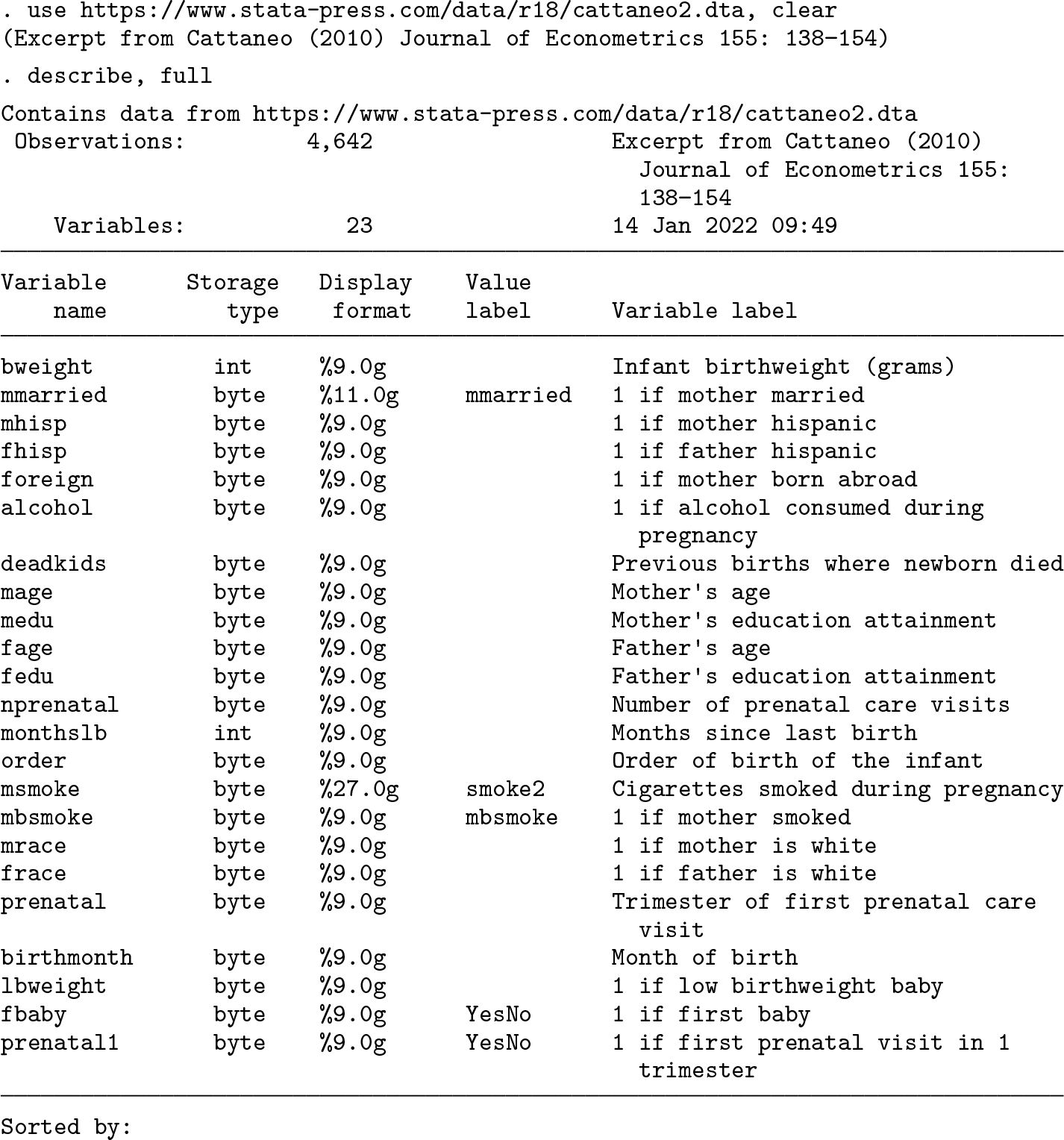
As an example, we use the dataset of Cattaneo (2010) (see [TE] teffects ipw), which has 1 observation for each of 4,642 pregnancies and data on self-reported maternal smoking status, child birthweight, and a list of candidate confounders that predict maternal smoking and might predict child birthweight. This dataset can be downloaded from within Stata and is described as follows:

We will concentrate on the binary maternal smoking status (mbsmoke) as a predictor of the child’s quantitative birthweight in grams (bweight). Of the 4,642 pregnancies, 864 (18.61%) involved mothers who admitted to smoking during pregnancy, and there were no missing values for birthweight. The other covariates will be used in a propensity model to predict maternal smoking during pregnancy.

In the Rubin causal model, we are allowed to find a propensity model by trial and error in the exposure and confounder data, as long as we apply it to the outcome data afterward and write it up for publication unconditionally on whether it gives the answer we wanted to hear. We want the propensity model to predict the exposure and, at the same time, to generate propensity weights that remove (or at least reduce) any imbalance in confounder values between the two exposure groups (self-reported smoking and nonsmoking mothers). We would also like this to be done in a way that does not lose too much power to detect a contrast in outcome between the exposure groups. And it is also important to define the kind of contrast that we aim to measure between the two exposure groups.

We will summarize our trial-and-error process by running the Rubin causal sequence for four candidate designs, based on the covariates of cattaneo2.dta. These designs, corresponding to four combinations of two design matrices and two propensity models, are as follows:

Original dataset (without outliers), logit model.

Original dataset, robit model with 2 d.f.

Outlier dataset (with one observation altered to produce an outlier), logit model.

Outlier dataset, robit model with 2 d.f.

(The 2 d.f. robit was itself chosen by trial and error, which we are allowed to do in the context of a Rubin causal design phase.) We will start by demonstrating the Rubin causal design phase in detail with the first design (original dataset, logit model) and then proceed to presenting the other designs in less detail. The methods used will be similar to those presented in Newson (2016).

We start by fitting the logit propensity model in the original dataset as follows:

We then compute the propensity score, which for each subject is equal to the estimated probability of smoking for that subject:

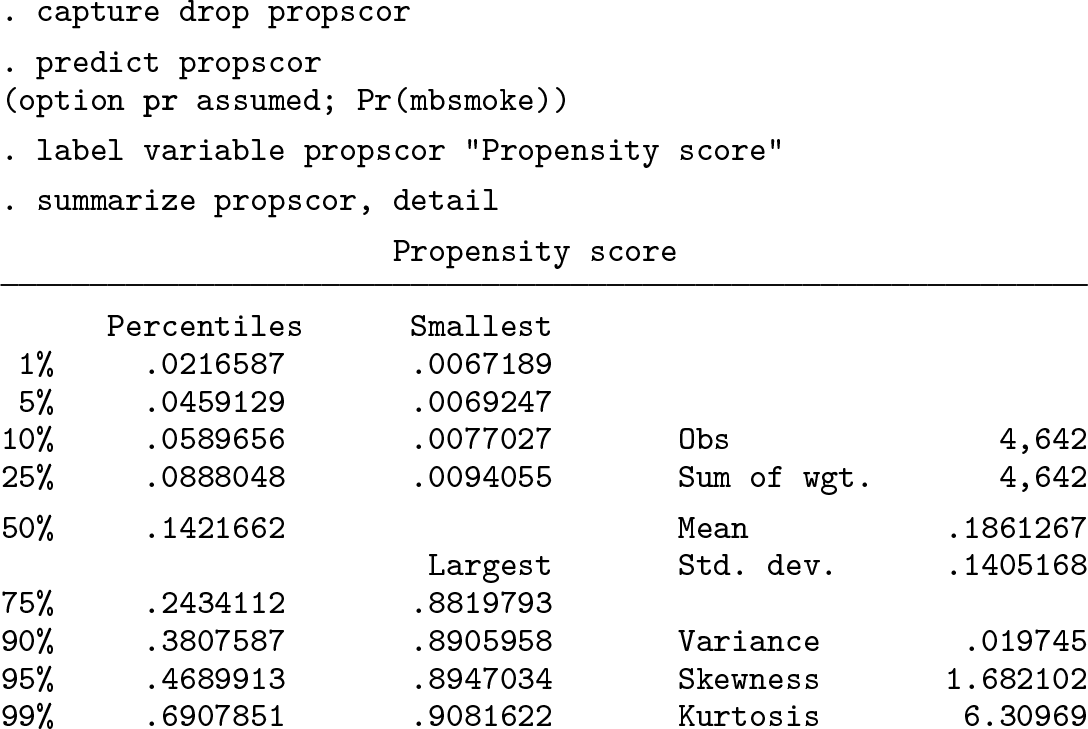
We see that subjects in the dataset have fitted probabilities of smoking ranging from 0.0067 to 0.9082. We would like to estimate average treatment effect (ATE) weights, sometimes known simply as inverse probability of treatment weights. These can be used to estimate the difference in mean birthweight between two fantasy scenarios defined as alternative versions of the dataset: one where all mothers admit to smoking during pregnancy and one where no mothers admit to smoking during pregnancy, both with other covariate values the same as in the original dataset. These weights are computed as follows:

We see that the propensity ATE weights vary from 1.007 to 38.671.

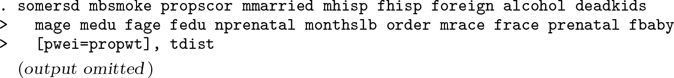
To check whether these weights balance out the association of smoking with the propensity score and its component covariates, we will use Somers’s D statistic for these associations, unweighted and weighted by the propensity ATE weights. Somers’s D is discussed in Newson (2006, 2002b) as an asymmetric measure of association, on a scale from −1 to 1, and related to Harrell’s c-index c(V |X) (also known as the receiver operating characteristic area of V with respect to X) by the formula D(V |X) = 2c(V |X)−1, where X is the binary exposure variable and V can be an outcome variable, a propensity score, or a confounder. In a propensity balance-checking context, it has advantages over the more commonly used standardized exposed-unexposed differences, used by official Stata’s teffects command (see [TE] teffects ipw) and by Lunt’s (2017) pbalchk package (found by typing findit pbalchk in Stata). In particular, under a wide variety of regression models, D(V |X) can be transformed to give a predictive treatment effect of X on V. For instance, if X and V are both binary, then D(V |X) is exactly the difference between Pr(V = 1|X = 1) and Pr(V = 1|X = 0). And if X is binary and V is conditionally equal-variance normal, with different conditional means for each value of X and a common standard deviation, and D(V |X) is between −0.5 and +0.5, then 2D(V |X) is approximately the difference between the conditional means given X = 1 and X = 0, expressed in units of the common standard deviation. And because D(V |X) is invariant under any monotone-increasing normalizing and variance-stabilizing transform on V, 2D(V |X) will be approximately the standardized difference between the corresponding conditional means of the transformed V. So either way, for a confounder or propensity-score W, a small propensity-weighted Somers’s D(W |X) can be used to give an upper bound to the spurious treatment effect on an outcome Y attributable to W because a larger D(Y |X) cannot be secondary to a smaller D(W |X) with the same sign. And a large propensity-weighted D(W |X) indicates a problem of nonoverlap, which our weighting has not balanced.

In our case, we measure the unweighted Somers’s D values of the propensity score and its component covariates with respect to the exposure, using the command

and the corresponding propensity-weighted Somers’s D values using the command

Instead of trying to digest the printed somersd (Newson 1998b) output, we will look at figure 3, which plots the unweighted and ATE-weighted indices against the propensity score and its component covariates. From the unweighted indices, we see that the propensity score predicts smoking positively and that its component covariates predict smoking positively or negatively. From the ATE-weighted indices, we observe that the ATE weights balance out most (but not quite all) of the predictive power, implying a limit to the potential spurious ATE attributable to residual confounding. Note that we have not included CIs and p-values, because we are not really worrying about whether these associations arose by chance. We are worrying about whether these associations could be primary to whatever exposure-outcome associations may be discovered once the outcome data are included.

Has the balancing power been won at the cost of inflating the CIs for the outcome effects? We can answer this question using the SSC package haif (Newson 2009a), which measures homoskedastic adjustment inflation factors (often known as variance inflation factors). We can measure variance inflation caused either by including confounders in an outcome model or by using the confounders to compute propensity weights, under the pessimistic assumption that the confounder adjustment is not really necessary, because the “confounders” predict only the exposure, not the outcome. General principles of variance inflation can be found in Seber and Lee (2003, chap. 3.7). In our case, we imagine that we will fit a regression model for birthweight with two parameters, namely, an intercept measuring average birthweights for babies with nonsmoking mothers and a smoking effect (the ATE) measuring the difference in average birthweights between smoking and nonsmoking mothers, with ATE-weighted Huber variances. The output produced is as follows:

The two columns of the listed output matrix contain inflation factors for the variances and SEs, respectively. And the two rows correspond to the two parameters estimated, namely, the smoking effect (the ATE) and the intercept estimating mean outcome for babies with nonsmoking mothers. We see that if the confounders predict only smoking and not birthweight, then, for the ATE, variances (and therefore sample numbers required for a specified power) will be inflated by a factor of 1.499, and SEs (and therefore CI widths) will be inflated by a factor of 1.224.

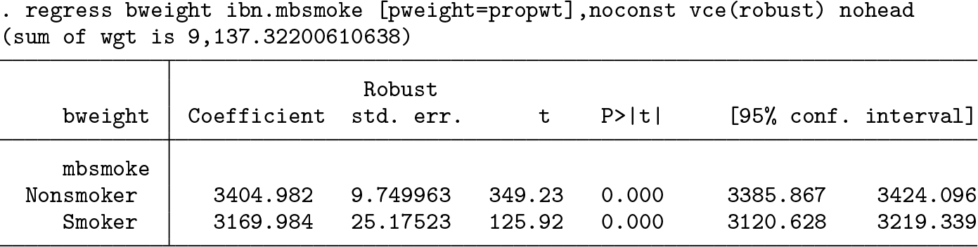
We might decide, in light of this design phase, to proceed to the analysis phase and to measure the effect of smoking on birthweight, adjusted for the confounders. If we do this, then we fit a regression model of the outcome bweight with respect to the exposure mbsmoke, using the ATE weights as probability weights, as follows:

The parameters here are the counterfactual scenario means for the dream scenario (where no mothers smoke) and the nightmare scenario (where all mothers smoke). We see that the mean birthweight is 3404.982 grams in the dream scenario and 3169.984 grams in the nightmare scenario. The nightmare-dream scenario difference is the ATE and can be estimated using the SSC package lincomest (Newson 2002a), a version of lincom that saves its results as estimation results. (This enables us to tabulate the estimates using the SSC packages parmest [Newson 1998a] and listtab [Newson 2009b].)

We see that the ATE is −234.998 grams (95% CI [−287.926 to −182.071 grams]). Note that the regression model is the same as the one assumed when we used haif but with a different initial parameterization (two scenario means). The most interesting parameter (the ATE) is the one estimated using lincomest.

Alternatively, we might not proceed immediately to the analysis phase but instead try out other designs. For the second design (original data, robit model), instead of using logit, we use robit with 2 d.f.:

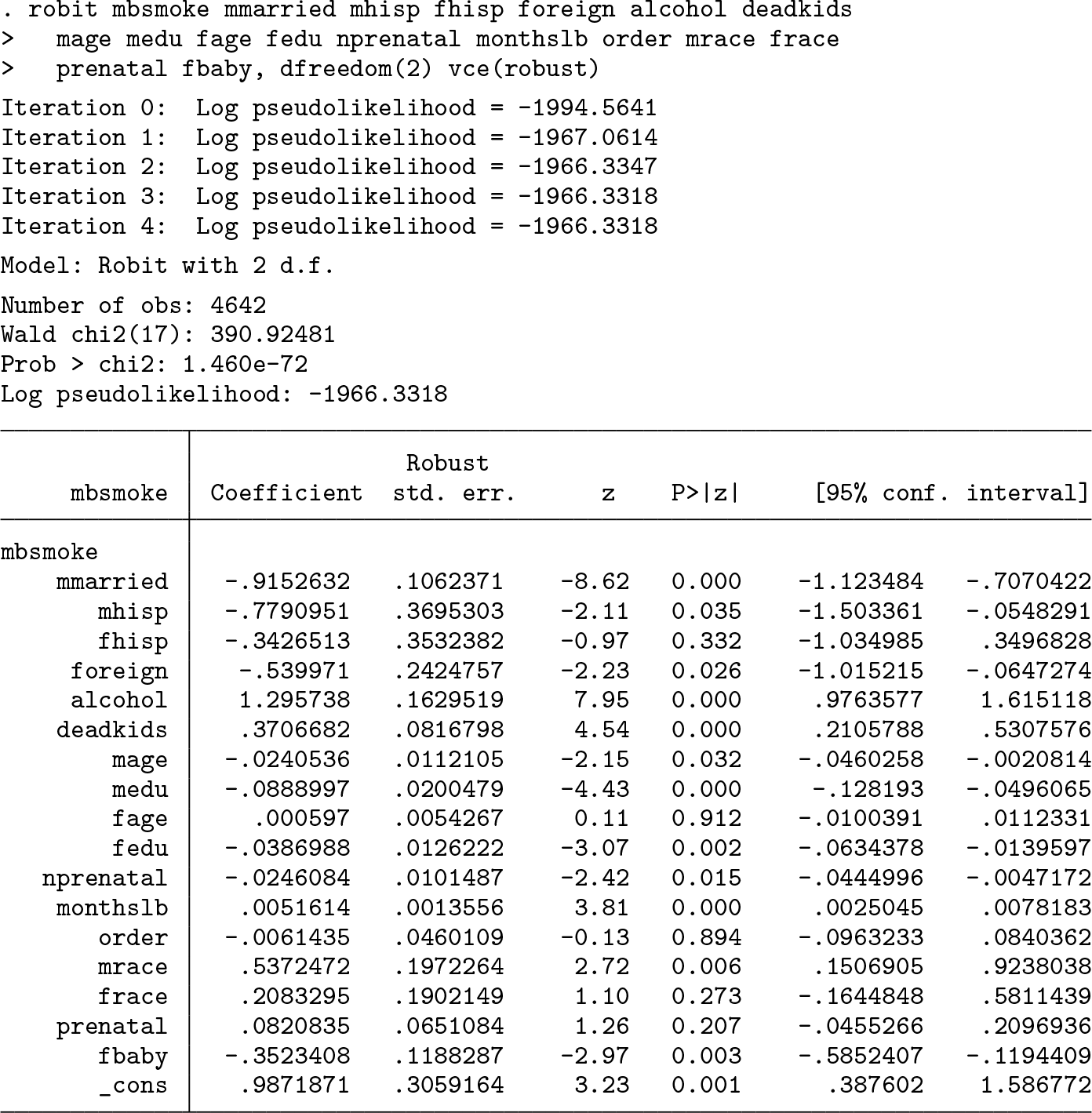
This time, the parameters are even harder to understand because they are expressed in robit units with 2 d.f. However, we can still compute propensity scores and ATE weights and do balance checks and variance inflation checks as before.

For the outlier designs, we identify a candidate outlier in the original dataset by choosing the subject with the lowest smoking propensity score under the logit model:

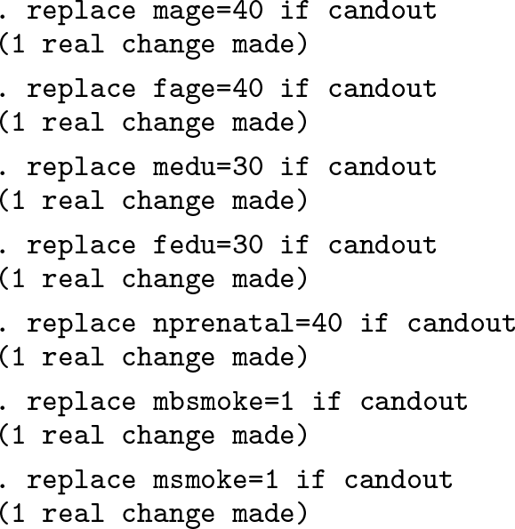
We see that the candidate outlier (identified by the indicator variable candout) is unique. To make the outlier dataset, we replace the values of a few variables in the outlier only, as follows:

We have revised this pregnancy (which already had a low smoking propensity) so that both the mother and father are 40 years old, have 30 years of full-time education (being perpetual students), and bother their doctor sufficiently to have 40 prenatal visits (the maximum observed in the original data). All of these features will probably predict high social and educational ranks and a low smoking propensity because people with such features do not often smoke. However, we then make them smokers. As very atypical smokers, they will probably have a high propensity ATE weight. (These fantasy parents are possibly living off trust funds and smoking ganja weed.) Having created our pregnancy record with exceptional but credible parents, we can rerun our logit and robit propensity models, doing the balance and variance inflation checks as before.

The balance checks for the four designs are done by plotting the unweighted and ATE-weighted Somers’s D statistics as reported in figures 3, 4, 5, and 6, respectively. We see that the robit model on the original dataset balances the propensity score and the covariates similarly to the logit model on the original dataset. However, the logit model on the outlier dataset is a disaster because a lot of weighted Somers’s D indices are large in either direction and the weighted Somers’s D for the propensity score is actually negative. The robit model on the outlier dataset, by contrast, balances the covariates and its propensity score similarly to the logit and robit models on the original dataset.

Figure 3.

Somers’s D indices with respect to maternal smoking under design 1

Figure 4.

Somers’s D indices with respect to maternal smoking under design 2

Figure 5.

Somers’s D indices with respect to maternal smoking under design 3

Figure 6.

Somers’s D indices with respect to maternal smoking under design 4

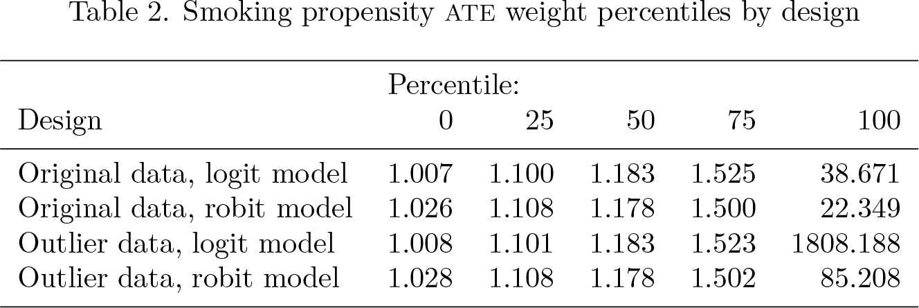
The smoking propensity-score percentiles for the four designs are given in table 1. The corresponding smoking ATE weight percentiles are given in table 2. We see that there is an enormous maximum ATE weight of 1808.188 for the logit model in the outlier dataset that belongs to our generated outlier. This is probably important in preventing these weights from balancing. By contrast, the maximum ATE weight for the robit model in the outlier dataset is “only” 85.208, which does not seem to compromise the balance.

Table 1.

Smoking propensity-score percentiles by design

	Percentile:
Design	0	25	50	75	100
Original data, logit model	0.0067	0.0888	0.1422	0.2434	0.9082
Original data, robit model	0.0257	0.0956	0.1397	0.2302	0.8992
Outlier data, logit model	0.0006	0.0899	0.1424	0.2422	0.8995
Outlier data, robit model	0.0117	0.0960	0.1401	0.2301	0.8972

Table 2.

Smoking propensity ATE weight percentiles by design

	Percentile:
Design	0	25	50	75	100
Original data, logit model	1.007	1.100	1.183	1.525	38.671
Original data, robit model	1.026	1.108	1.178	1.500	22.349
Outlier data, logit model	1.008	1.101	1.183	1.523	1808.188
Outlier data, robit model	1.028	1.108	1.178	1.502	85.208

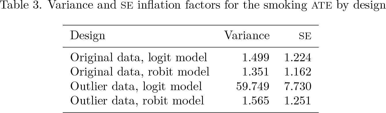
The variance inflation factors for the smoking ATE are given in table 3. These are nonspectacular for all sets of weights except for the weights from the logit model in the outlier scenario. The problem here is probably the outlier again. Outliers may or may not compromise the balance but usually inflate the variance, at least if the covariates predict only the exposure and not the outcome conditionally on the exposure.

Table 3.

Variance and SE inflation factors for the smoking ATE by design

Design	Variance	SE
Original data, logit model	1.499	1.224
Original data, robit model	1.351	1.162
Outlier data, logit model	59.749	7.730
Outlier data, robit model	1.565	1.251

Based on these design-stage results, we might choose to proceed to the analysis stage with either the robit or the logit for the original dataset, but we would definitely prefer the robit for the outlier dataset. So the robit seems to rein in the effect of outlying pregnancies without doing any damage in the absence of outlying pregnancies.

The ATE estimates for smoking on birthweight in grams for the four designs (with confidence limits and p-values) are reported in table 4. These are all similar to each other, except for the one for the logit model in the outlier dataset, which we would have rejected in the design phase.

Table 4.

Smoking ATE estimates for birthweight (grams) by design

Design	ATE	[95% CI]	P
Original data, logit model	−234.998	[−287.926, −182.071]	4.4 × 10 ⁻ ¹⁸
Original data, robit model	−236.552	[−286.111, −186.993]	1.2 × 10 ⁻ ²⁰
Outlier data, logit model	−456.157	[−764.952, −147.362]	0.0038
Outlier data, robit model	−251.693	[−307.925, −195.461]	2.4 × 10 ⁻ ¹⁸

5 Conclusions

We have developed a new user-friendly command (robit) for robit regression and made available a set of community-contributed robit link functions (via the SSC package xlink) to be used with the glm command. This fills a gap in the preexisting capabilities of Stata.

Robit models have been described in the literature as a simple robust alternative to logistic and probit models. In particular, they have been recommended for the estimation of inverse-probability weights to adjust for missing-at-random values or for deriving propensity scores for causal inference. Further work to evaluate the performance of robit models under various scenarios in these settings would be helpful.

We hope that our robit and xlink packages will be valuable additional tools in Stata and will also promote sensitivity analyses and further simulation studies.

7 Programs and supplemental materials

Supplemental Material, sj-zip-1-stj-10.1177_1536867X231195288 - Robit regression in Stata

Supplemental Material, sj-zip-1-stj-10.1177_1536867X231195288 for Robit regression in Stata by Roger B. Newson and Milena Falcaro in The Stata Journal

Footnotes

6 Acknowledgment

This article has benefited from helpful discussions with our colleague Professor Peter Sasieni of King’s College London.

7 Programs and supplemental materials

To install a snapshot of the corresponding software files as they existed at the time of publication of this article, type

References

Albert

J. H.

Chib

. 1993. Bayesian analysis of binary and polychotomous response data. Journal of the American Statistical Association 88: 669–679. https://doi.org/10.2307/2290350.

Buis

M. L.

2007. Stata tip 48: Discrete uses for uniform(). Stata Journal 7: 434–435. https://doi.org/10.1177/1536867X0700700309.

Cattaneo

M. D.

2010. Efficient semiparametric estimation of multi-valued treatment effects under ignorability. Journal of Econometrics 155: 138–154. https://doi.org/10.1016/j.jeconom.2009.09.023.

Gelman

Hill

Vehtari

. 2021. Regression and Other Stories. Cambridge University Press: Cambridge. https://doi.org/10.1017/9781139161879.

Kang

J. D. Y.

Schafer

J. L.

. 2007. Demystifying double robustness: A comparison of alternative strategies for estimating a population mean from incomplete data. Statistical Science 22: 523–539. https://doi.org/10.1214/07-STS227.

Lange

K. L.

Little

R. J. A.

Taylor

J. M. G.

. 1989. Robust statistical modeling using the t distribution. Journal of the American Statistical Association 84: 881–896. https://doi.org/10.2307/2290063.

Nadarajah

. 2020. A review of Student’s t distribution and its generalizations. Empirical Economics 58: 1461–1490. https://doi.org/10.1007/s00181-018-1570-0.

Liu

C. H.

2004. Robit regression: A simple robust alternative to logistic and probit regression. In Applied Bayesian Modeling and Causal Inference from Incomplete-Data Perspectives, ed. Gelman

Meng

X.-L.

, 227–238. Chichester, U.K.: Wiley. https://doi.org/10.1002/0470090456.ch21.

Liu

C. H.

2006. Robit regression: A simple robust alternative to logistic and probit regression. https://www.stat.purdue.edu/∼/chuanhai/teaching/Stat598A/robit.pdf.

10.

Lunt

2017. Propensity analysis. https://personalpages.manchester.ac.uk/staff/mark.lunt/propensity.html.

11.

McCullagh

Nelder

J. A.

. 1989. Generalized Linear Models. 2nd ed. London: Chapman and Hall/CRC. https://doi.org/10.1201/9780203753736.

12.

Mudholkar

G. S.

George

E. O.

. 1978. A remark on the shape of the logistic distribution. Biometrika 65: 667–668. https://doi.org/10.1093/biomet/65.3.667.

13.

Newson

R. B

. 1998a. parmest: Stata module to create new data set with one observation per parameter of most recent model. Statistical Software Components S352601, Department of Economics, Boston College. https://ideas.repec.org/c/boc/bocode/s352601.html.

14.

Newson

R. B

. 1998b. somersd: Stata module to calculate Kendall’s tau-a, Somers’ D and median differences. Statistical Software Components S336401, Department of Economics, Boston College. https://ideas.repec.org/c/boc/bocode/s336401.html.

15.

Newson

R. B

. 2002a. lincomest: Stata module to generate linear combinations of estimators saved as estimation results. Statistical Software Components S430901, Department of Economics, Boston College. https://ideas.repec.org/c/boc/bocode/s430901.html.

16.

Newson

R. B

. 2002b. Parameters behind “nonparametric” statistics: Kendall’s tau, Somers’ D and median differences. Stata Journal 2: 45–64. https://doi.org/10.1177/1536867X0200200103.

17.

Newson

R. B

. 2006. Confidence intervals for rank statistics: Somers’ D and extensions. Stata Journal 6: 309–334. https://doi.org/10.1177/1536867X0600600302.

18.

Newson

R. B

. 2009a. haif: Stata module to compute Homoskedastic Adjustment Inflation Factors for model selection. Statistical Software Components S457016, Department of Economics, Boston College. https://ideas.repec.org/c/boc/bocode/s457016.html.

19.

Newson

R. B

. 2009b. listtab: Stata module to list variables as rows of a T_EX, HTML or word processor table. Statistical Software Components S457088, Department of Economics, Boston College. https://ideas.repec.org/c/boc/bocode/s457088.html.

20.

Newson

R. B

. 2016. The role of Somers’ D in propensity analysis. Presented at the U.K. Stata Users Group meeting, London, U.K., September 8–9. https://www.stata.com/meeting/uk16/slides/newson_uk16.pdf.

21.

Newson

R. B

. 2021. xlink: Stata module to provide extra link functions for use with glm. Statistical Software Components S458996, Department of Economics, Boston College. https://econpapers.repec.org/software/bocbocode/s458996.htm.

22.

Ridgeway

McCaffrey

D. F.

. 2007. Comment: Demystifying double robustness: A comparison of alternative strategies for estimating a population mean from incomplete data. Statistical Science 22: 540–543. https://doi.org/10.1214/07-STS227C.

23.

Rubin

D. B.

2008. For objective causal inference, design trumps analysis. Annals of Applied Statistics 2: 808–840. https://doi.org/10.1214/08-AOAS187.

24.

Seaman

S. R.

White

I. R.

. 2013. Review of inverse probability weighting for dealing with missing data. Statistical Methods in Medical Research 22: 278–295. https://doi.org/10.1177/0962280210395740.

25.

Seber

G. A. F.

Lee

A. J.

. 2003. Linear Regression Analysis. 2nd ed. New York: Wiley. https://doi.org/10.1002/9780471722199.

26.

Zellner

1976. Bayesian and non-Bayesian analysis of the regression model with multivariate Student-t error term. Journal of the American Statistical Association 71: 401–405. https://doi.org/10.1080/01621459.1976.10480357.

Supplementary Material

Please find the following supplemental material available below.

For Open Access articles published under a Creative Commons License, all supplemental material carries the same license as the article it is associated with.

For non-Open Access articles published, all supplemental material carries a non-exclusive license, and permission requests for re-use of supplemental material or any part of supplemental material shall be sent directly to the copyright owner as specified in the copyright notice associated with the article.

0.00 MB