






Abstract
The defeat of a swarm of uncrewed aerial systems is an important problem for current fighting forces. The purpose of this paper is to develop a simplified framework in which the defeat of such a swarm may be quantified. This is in the context where area surveillance is provided by an
1. Introduction
1.1. Context and objectives
This paper is concerned with the operational effectiveness of directed energy weapons (DEWs) applied for counter uncrewed aerial system (CUAS) defeat. Countering of swarms of uncrewed aerial vehicles (UAVs) is a problem of considerable importance in modern warfare.1–4 The main focus here is on high energy laser (HEL) DEW performance when protecting a region against such threats. 5 However, the analysis may be applied to other DEW effectors such as high power radio frequency (HPRF) systems. HEL DEWs are an effective solution to the CUAS problem, since they can provide precision strikes at considerable distances with near speed of light engagement times.6–8
The approach adopted in this study is a simplified version of the kill chain of threat detection, classification, tracking, engagement decision making and effecting. It develops a mathematically driven model to quantify integrated sensing and effecting for CUAS effectiveness. This basic model yields some insights into integrated defensive system performance under a number of operational conditions and threat parameters.
From a sensing perspective, swarms of UAVs present a challenge because they may consist of low radar cross section (RCS) targets making them difficult to detect. Due to the fact that UAV propellers admit a micro-Doppler signature, Doppler processing, in addition to amplitude-based detection, has been shown to enhance radar performance in detecting UAVs. 9 These micro-Doppler signatures have also been used as a basis for detection from a continuous-wave coherent lidar. 10 In addition, there have been applications of acoustic systems for UAV detection, since the latter emits acoustic waves. 11 Although the focus in this paper is on amplitude-based radar detection, there is scope to extend the analysis to other sensor systems such as those outlined above.
HEL DEWs require a dwell time in which to induce thermal damage on targets, resulting in detected threats requiring a waiting time for processing by the effector. Given a swarm of UAVs is not likely remaining stationary, these UAVs may be converging onto their target while the HEL is processing the current threat. This potential delay in processing threats may result in at least one UAV reaching its intended target. Hence, it is important to understand a DEW system’s performance when it is facing a swarm of UAVs, especially the nature of its processing delays.
An integrated sensing and effecting system will have threats cued through the sensing process, which can be complex for DEWs. If the effecting mechanism does not introduce waiting times for processing, then threats will be acted on by the DEW once they are in its effective range. This is the case for HPRF DEWs and laser dazzlers. In the HEL, DEW situation threats will inevitably experience a waiting time. The approach developed in Weinberg, 12 and extended in Weinberg, 13 assumes that threats arrive into the theater of operation through a renewal process. This then permits HEL performance to be modeled through a single-server queue, where the service times correspond to that taken to neutralize the current threat and delays experienced by waiting threats may be modeled through a recursive relationship. 14 Although this is a valid approach, it becomes difficult to introduce an analytically tractable solution when the arrival process is determined through a sensing mechanism. Even if detection of threats is assumed independent, the interarrival times are not independent, resulting in complexity in adapting the queuing framework for delay processing as discussed in Ross. 14 This is further complicated by the fact that it becomes necessary to consider the ranked order of threat arrivals, requiring the application of order statistics (OS). Although the joint density of such OS may be constructed, when combined with variations of the delay structure in Ross, 14 the resulting expressions for performance prediction are not useful in practice. Hence, it became necessary to develop a new framework in which HEL DEW performance may be assessed when a sensing process is generating the arrival distribution.
Therefore, the main objective of this paper is to develop a preliminary model to account for integrated sensing and effecting without dealing with the complexity of queuing theory models. Under a restriction on the behavior of the UAVs, a new approach is developed to allow detection times to replace the assumption of arrivals into the theater of operation through a renewal process. Metrics for both BLUFOR and REDFOR mission success will be introduced, which will be based upon OS of detection times that will then permit some insights into expected system performance.
1.2. UAVs in modern warfare
In modern warfare the application and use of UAVs is becoming prevalent.15,16 The initial use of UAVs in military settings was for intelligence, surveillance, and reconnaissance purposes; however, their utility as a weapon has also emerged. 17 As reported in the latter, countries including the United States, United Kingdom, Israel and Italy were among the first to see the potential in developing weaponized drones. For an example of a large-scale UAV, General Atomics developed the MQ-9 Reaper, which can be equipped with Paveway laser guided bombs and AGM-114 Hellfire missiles. It has been deployed by the US Air Force for over a decade, and has been used extensively for precision strikes. 18 Smaller UAVs have also been used to attack military targets, an example being the frequent attacks on the Russian Hmeymim Air Base in Syria. As a particular instance of this, on 6 January 2018, 13 combat fixed-wing UAVs attacked this base, launched by terrorists. 17
The ongoing war in Ukraine has also demonstrated the utility of UAVs in contemporary conflicts and the need for effective countermeasures. 19 What one observes from this war is that UAVs can be used to provide an asymmetric advantage. The conflict has also demonstrated the utility in utilizing commercial off-the-shelf (COTS) UAVs in warfare. As is discussed in Molloy, 20 small weaponized UAVs have provided Ukraine with the ability to deploy a cheap weapon to strike targets remotely while preserving the safety of the operator and providing the enemy with a difficult to detect threat. Ukraine has used small swarms of UAVs to destroy armored convoys in the Donetsk Region, 21 while Russia has deployed Iranian Kamikaze drones (loitering munitions) to attack Ukrainian infrastructure. 22 Both forces in this conflict have had to develop their tactics, techniques, and procedures (TTP) for UAV usage as the war evolves, with Ukraine taking the lead in utilizing COTS UAVs to defend against a stronger aggressor.
1.3. Modeling approach and assumptions
There are quite a number of studies investigating the problem of UAV swarms and their neutralization. Examinations of swarms and the interaction between members are considered in Tahira et al., 23 Castrillo et al., 24 and Chang et al., 25 while Seidaliyev et al. 26 provide an overview of the issues concerning detection and classification. The way in which UAV swarms may be used to attack targets, and their neutralization, is overviewed in Chamola et al. 17
As is discussed in Castrillo et al., 24 there are a number of ways in which a group of UAVs may be configured, based upon collaboration between members. The four main formations can be described as follows:
In this study, a combination of the latter two will be adopted in the analysis. In particular, it will be assumed that a collection of UAVs are converging on a target, such that they are traveling at the same speed but may differ in spatial position initially as well as their electromagnetic signature. The assumption of common speed results in the group/swarm remaining in a coherent pattern throughout. Otherwise, the collection of UAVs may be categorized as groups of isolated individuals as well as a core team/swarm.
This analysis will focus on small COTS UAVs resulting in smaller weight, speed, and RCS assumptions. These UAVs, classified as NATO class 1 and 2, have featured significantly in the Russian−Ukrainian War. 27 They tend to weigh up to 24 kg, and travel at maximum speeds ranging from 13 to 30 m/s. 28 As discussed in Gong et al., 9 group 1 UAVs, as classified by the US Department of Defense, generally have an RCS of between 0.01 and 0.1 m2.
The tactics employed include coordinated strikes to targets, enhanced by a large number of swarm members. Specifically, a swarm may be directed toward an airfield to disrupt air traffic and to attack critical infrastructure. A series of low-flying UAVs may be used to strike a convoy of vehicles, as mentioned previously. The fact that they may be operated autonomously and can exhibit complex decentralized behavior can result in them becoming a difficult threat to counter. 17 For the purposes of this study, it will be assumed that the swarm is converging onto its target without complex individual motion.
It is important to note that the solution proposed in this paper is contingent on a common speed assumption, otherwise it becomes necessary to re-prioritize detected UAVs for processing by the HEL DEW. For brevity, the term swarm will be used to encompass both teams/swarms as defined above.
From a sensing perspective, a number of modeling simplifications will be adopted. It will be assumed that the existence of the swarm has been established, that it has been classified as consisting of potential threats, and is being tracked by the sensor system which has passed onto the DEW the necessary engagement information to allow it to act. Since these threats will have been determined to be traveling at the same speed, the engagement decision process will be to neutralize threats in the order in which they have been detected. This simplified command and control mechanism will only work under the assumptions adopted in this paper. The conclusions will discuss future research efforts which will address this limitation.
2. Performance models
Throughout this study, units of distance and wavelength will be measured in meters (m), time in seconds (s) and speed in meters per second (m/s). RCS will be in square meters (m2). Irradiance is measured in Watts per square meter (W/m2) with the same units applied to thermal disruption thresholds.
2.1. Generic model development
Suppose that there are
It is necessary to distinguish between arbitrary labeling of threats and the order in which they are detected by the sensor network. Hence, the
Figure 1 provides an illustration of the combat scene, from a two-dimensional perspective. In this example, the one DEW (denoted
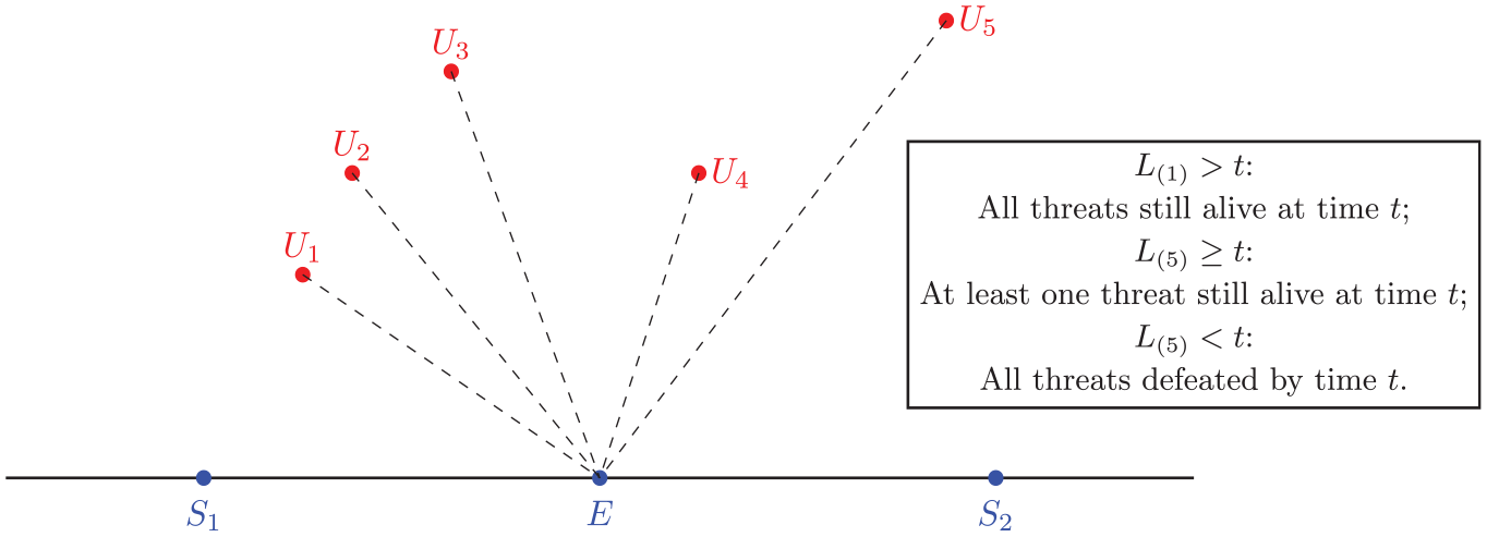
An illustration of the combat scene, where a series of five threats are converging onto the DEW (denoted
What is now required is a statistical model for the lifetime distribution of the last detected threat. It is worth noting that the following analysis may be used to construct a model for the lifetime of the first detected threat if of interest in numerical analysis.
Note that the event
under the assumption that detection of threats is independent, where
Consider the last detected threat, which is detected at time
One may utilize Equation (1) to simplify Equation (2), and what is then required is the probability that this threat is not neutralized in the observational window
since this threat enters service at time
where Equation (1) may then be utilized in the above. In this analysis, the parameters
It is informative to note that in order to ensure that the argument of the second distribution function in Equation (4) is non-negative one must impose the condition
which provides a time-dependent upper bound on the maximal permissible delay.
In order to evaluate Equation (4), one requires the parameter set
For the initial arbitrary ranking of threats, suppose that the sequence
where
Expression (6) enables one to produce a probability distribution of the last detected threat’s position in the sequence of detection times, and then permits the specification of relevant parameters in Equation (4). A useful way in which Equation (6) may be evaluated is through Monte Carlo simulation. Since
and one may apply the inverse cumulative distribution function method to simulate
To summarize this section the modeling framework is illustrated in Figure 2, indicating how one may use it to inform system specifications to ensure a desired level of operational effectiveness against a given threat class. The probability of defeating the swarm is labeled metric 1, while its complement is metric 2.

The modeling framework and how it is used to inform system design. From integrated system configurations and a given threat class, one may use the framework to assess operational effectiveness and then use it to inform the design of a CUAS solution for specific threat classes.
2.2. Sensing through an X-band radar
In order to apply the above what is required is a model for sensor performance. Hence, an example is adapted from Mahafza,
29
specifically example 3.1 together with the signal-to-noise ratio (SNR) given by (3.16) in the latter but with no radar losses. Consequently, it will be supposed that each radar is
where
where
2.3. Effecting through a HEL
For the numerical analysis to follow it will be assumed that the DEW is a HEL, which may be functioning in a scenario where threats may be delayed before processing. It will be supposed that the laser operates in an environment where atmospheric effects are minimized, so for example thermal blooming will be considered compensated for through adaptive optics. Under the assumption of a Gaussian beam profile, the irradiance (5.11) from Weinberg 13 is adopted. This is given by
where
Throughout the following specific parameterizations will be adopted:
Note that in view of Equation (10), it follows that
4. Performance examples
A series of examples is now considered to illustrate the application of the main results. Throughout the following, a two-dimensional setting is taken for the study, where the HEL DEW is located at (0, 0) and two sensors are positioned at (−10, 0) and (10, 0), respectively. It will be assumed that the threats are converging onto the DEW’s position and arrive at different angles of arrival, as illustrated in Figure 1. Each case considered will discuss the example’s variation in threat parameters.
In terms of the delay which the last detected threat may experience, the following choice is adopted. Based upon considerations in Burley
32
and Puent,
33
the time it takes to cause a thermal disruption will be in the order of seconds depending on the UAV’s hardening to thermal effects. Hence, as an approximation, it will be assumed that it takes about 3 s to cause a thermal effect. Since we are concerned with the delay the last detected threat can experience, this will be maximal if all threats are detected simultaneously and all are placed in a queue for processing by the HEL DEW. Therefore, if there are
4.1. Case 1
For this case, it is assumed that the swarm consists of five identical UAVs, originating at the same distance and traveling at the same speed, with common RCS. Hence,
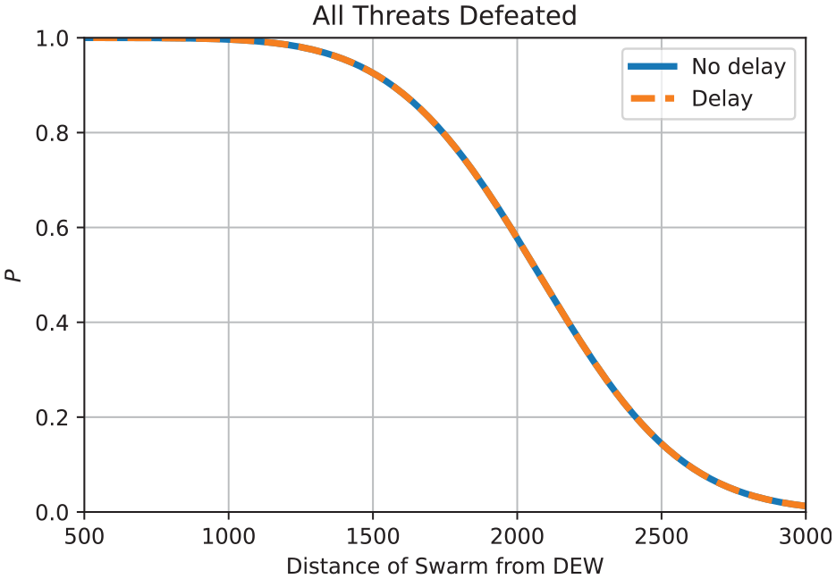
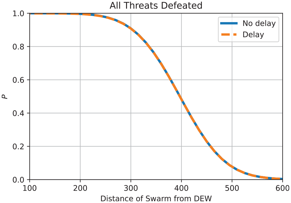
A plot for the case where
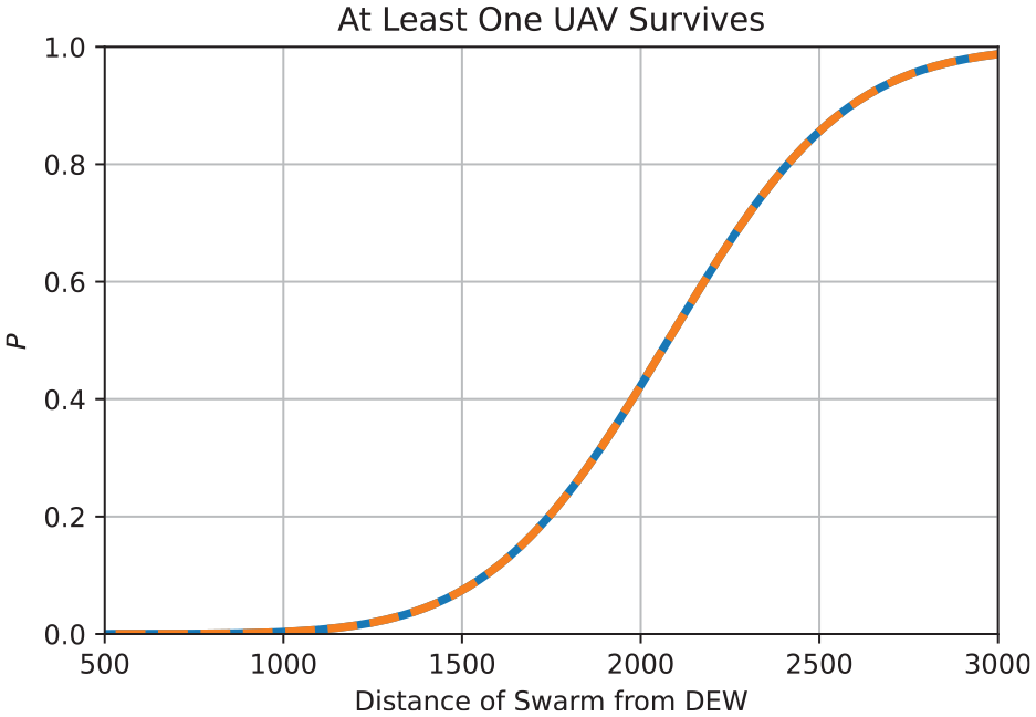
The complement of the plot in Figure 3 showing the probability that at least one swarm member survives as a function of distance to the DEW.
In this same scenario, when the common RCS is reduced to 0.01 m2, all threats will be defeated when the swarm is 500 m from the DEW, since the smaller RCS means that they take longer to detect but there is sufficient time to neutralize the swarm regardless of the delay (figure not include for brevity).
For the remaining examples, only plots of metric 1 will be included since that for metric 2 is simply the complement, as illustrated above.
Next consider the case where
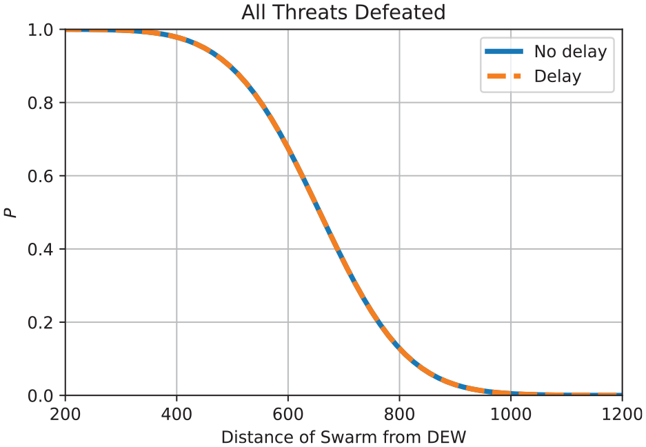
Probability of defeat for
It is interesting to explore the impact of faster traveling threats in the situation of Figure 5. In particular, when the common UAV speed is increased beyond 30 m/s one begins to see the impact of the delay on performance. At
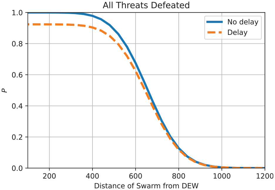
Effects of increasing UAV speed for the same situation as in Figure 5. Here
Obviously, the initial positioning of the swarm will have a significant impact on the DEW’s performance. To explore this further consider the case where
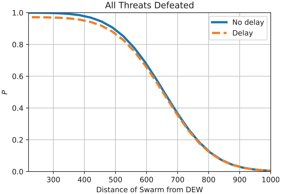
Exploring the impact of smaller
To explore this further, in Figure 8 the speed has been increased to 45 m/s, so that the threats are at a distance of 1.35 km from the DEW initially. Here there is a more severe difference between the delay and non-delay case. When the speed is increased to 50 m/s the probability of defeat of the swarm, when accounting for delays, reaches 0.7 at its maximum, as shown in Figure 9. In the latter case, the swarm is located at a distance of 1.8 km from the DEW initially.
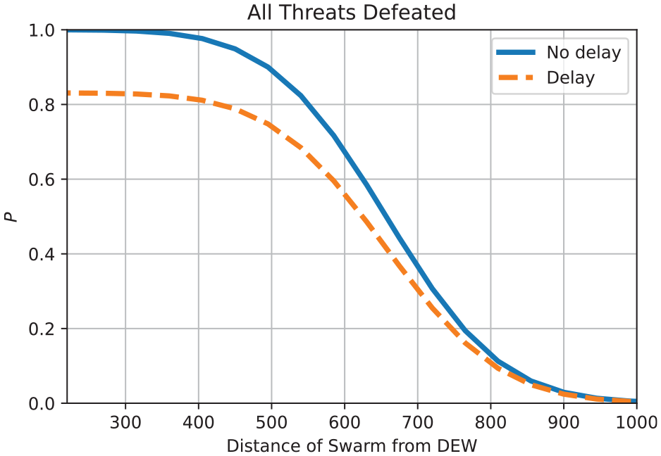
Scenario of Figure 7 with a speed of 45 m/s.
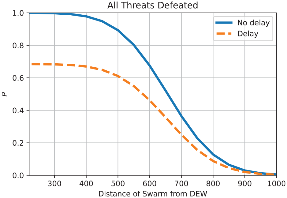
Another example of the effect of speed on the delay case, where the threats are traveling at 50 m/s.
It is important to note that the speeds used in Figures 7–9 are a bit excessive for COTS UAVs but this has been an important exercise since it illustrates potential problems when swarm members are traveling somewhat fast, with small RCS. However, with larger RCS, it can be shown that this situation improves, since faster traveling threats will be detected sufficiently early. As an example, when the RCS is increased to unity with a speed of 50 m/s in this case all threats will be defeated before they are within 1.2 km of the DEW, regardless of the delay.
4.2. Case 2
In this subsection, some examples are considered where the
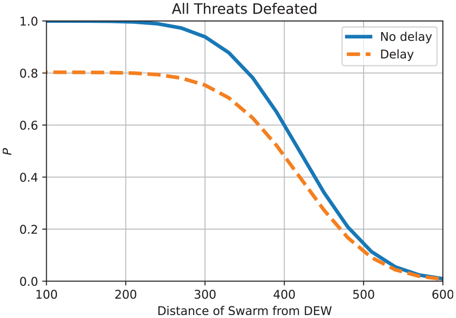
A study of the varying
Repeat of the scenario in Figure 10 except where threats travel at 30 m/s.
The example of this section showed that if the threats originate at different positions, then in the delay case one might see REDFOR achieving its mission objective at considerably smaller speeds than that illustrated in the previous subsection.
4.3. Case 3
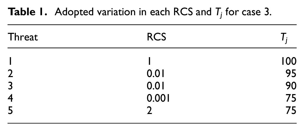
This section shows an example where variation in both the RCS and
whose
Adopted variation in each RCS and
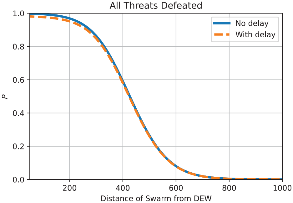
Variation in the RCS and
When all threat speeds are increased, one can see the impact of the delay. Figure 13 is when the common speed is increased to
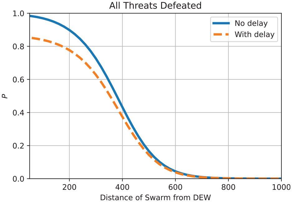
Scenario of Figure 12 with a speed of 20 m/s.
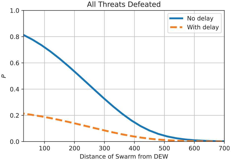
Consequences of a common speed of 30 m/s for the scenario of Figure 13.
In this example, there are two threats with large RCS and three with smaller RCS, so once they are traveling fast it is likely that the sensing network will not detect them with sufficient time to result in a successful disruption by the DEW, as the results have indicated. If a maximal delay is experienced then this results in REDFOR more likely to achieve its mission aims. The faster speeds utilized here are significantly slower than in the previous subsections, indicating variations in the RCS and points of threat origin can have a significant impact on BLUFOR mission success.
4.4. Case 4
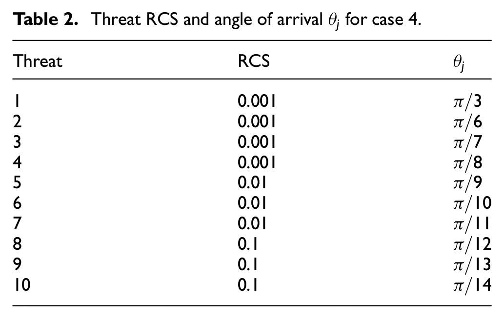
As a final example, the case where there are 10 threats in the swarm is considered, such that their parameters are given in Table 2. Since there are 10 threats the maximum delay is
Threat RCS and angle of arrival
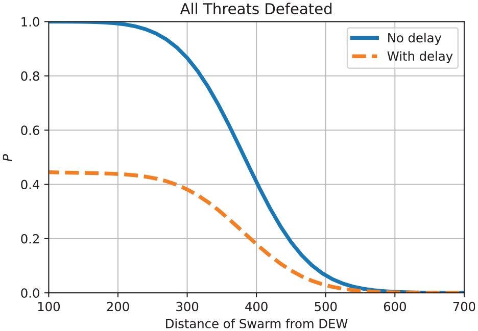
Performance when facing a swarm of 10 low RCS UAVS, flying at 15 m/s.
4.5. Some considerations
The previous example highlighted the impact that increased delay can have on expected performance. If instead of the maximum delay one assumed that
To ensure in practice that this delay is minimized, there are several potential solutions. In the first instance increasing the radar’s power, and the number of available sensors, will result in earlier detection of threats, which will then provide the DEW with more time to neutralize threats. Second, the DEW’s power may be increased to reduce the dwell time, provided there is compensation for atmospheric attenuation. This alone would be sufficient to ensure the delay of the last detected threat is below the limit required to ensure BLUFOR mission success.
Note that with reference to Equation (4), if one wanted to obtain bounds on the difference between this expression and the non-delay case, the key term is the second one in this expression, namely
The difference between Equation (11) and the non-delay case may be bounded by utilizing the mean value theorem. In particular, it can be shown that
where the function
and
and
Suppose that it is desired to ensure that the difference between the delay and non-delay cases is bounded by an arbitrary amount. Then from Equation (13), one may deduce the bound required on the delay in order to ensure this requirement. Calculations for the example mentioned in this discussion showed that the delay is bounded by a constant multiple of a power of the ratio of the square of the threat speed to its RCS and a product of three functions of the SNR. When the laser power to square speed ratio is increased, this bound also increases, implying that increasing laser power for slower moving targets will result in larger permissible delays. The bound is also reduced for larger RCS and slower traveling UAVs, which is a result consistent with observations made in the numerical analysis. Further mathematical exploration is required to further quantify bounds on Equation (13) in terms of system parameters.
5. Conclusions and future work
The purpose of this paper was to demonstrate how performance metrics for CUAS may be constructed for the case where sensing is provided by a network of
The analysis presented in this paper has indicated the need for further exploration of the problem of assessing integrated defensive system performance through mathematical models. First, since the swarm may contain UAVs which deviate from the assumed uniform speed it is necessary to examine how this can be accounted for in a performance assessment model. One approach may be to introduce a time-dependent threat ranking process, which schedules threats based upon the expected times they are likely to reach their intended targets. This may require a re-examination of the queuing theory approach of Weinberg 12 with the introduction of priority queuing. A second important requirement is the validation of adopted models through analysis of trials data with real operational systems and with a variety of UAVs, operating under various conditions. These two principal lines of effort will form the basis for subsequent future work.
Footnotes
Acknowledgements
The author would like to thank the two reviewers for their comments which provided practical insights into the complexity of UAV swarm defeat. The reviewers’ comments not only improved the current paper but have provided the author with important future research directions.
Declaration of conflicting interests
The author has declared no potential conflicts of interest with respect to the research, authorship, and/or publication of this article.
Funding
This research received no specific grant from any funding agency in the public, commercial, or not-for-profit sectors.
