A Stackelberg framework for disrupting coordinated,multi-asset routing and sequential servicing of demands

Abstract

This research examines the problem of routing multiple assets of different types over a network to service demands, where the demands must be serviced by asset types in sequential order within a bounded amount of time, and minimizing the cumulative service time is of interest. Disrupting these decisions, an opponent seeks to identify effective network disruption strategies with limited resources to maximize the minimal cumulative service time. Within a bilevel programming structure for this Stackelberg game, the upper-level problem determines the disruption strategy, and the lower-level problem routes the assets. Seeking the identification of high-quality solutions with relatively low computational effort, this research identifies and tests three solution procedures: a greedy construction heuristic (GCH) that iteratively identifies each disruptive action, a customized implementation of simulated annealing (SA), and an enhanced variant thereof (eSA) that leverages a prioritized identification of candidate solutions along with a tabu list. Testing compares the solution methods on similar instances over a range of selected algorithmic and instance-specific parameters. Results showed the enhanced SA method performed best, and extended testing explored the effect of increasing selected problem sets on the relative improvement in eSA over GCH, as well as its effect on algorithmic runtimes.

Keywords

multi-agent routing bilevel programming network interdiction simulated annealing game theory

1. Introduction

Consider a military scenario wherein an adversary has intelligence regarding the location of several assets they seek to destroy. First, intelligence, surveillance, and reconnaissance (ISR) assets must validate current intelligence, strike assets (e.g. aircraft and vehicles), move to the locations, and deliver munitions to destroy the targets. Such a process to “service demands” is also necessarily sequential in nature. In a defensive posture, we seek to conduct localized electronic interference, an aspect of an anti-access/area denial (A2/AD) environment.^1,2 This communication interference can increase travel time in targeted areas of a network, as up-to-date information cannot be refreshed or confirmed. The desired effect of these actions is to delay the adversary’s attacks and provide time to move or protect their targets from destruction. Thus, it is of interest to identify where to apply electronic interference most effectively.

Alternatively, consider the following motivating civil scenarios. Commodities are being transported to major construction efforts across a region. They require delivery in a timely manner to various sites, and their delivery sequence is relevant (e.g. concrete before framing material, then electrical conduits and outlets, after which the wallboard arrives). Traffic congestion can slow traffic on portions of potential delivery routes. Such delays can disrupt scheduled deliveries. Yet, knowing the locations where delays are most impactful and rerouting is not helpful will inform where mitigating actions (e.g. dedicated, on-site traffic control and the establishment of priority lanes) have merit.

Similarly, after a natural disaster or heavy storm, some capabilities or commodities should be delivered as assistance to impacted towns before others (e.g. rescue equipment and medical assistance are needed before building repair materials). Road network conditions may be degraded, making travel over certain road segments take more time. Understanding where road damage would be most impactful can inform decisions regarding where to stage a limited road repair capability.

Generalizing these related scenarios, this research explores the problem of a defender disrupting the routing of different types of assets having disparate but complementary capabilities (or commodities to deliver) over a directed network to service a set of demands sequentially. Given $n$ asset types, an asset of each type must visit a demand to service it, with Type $1$ visiting no later than Type $2$ , Type $2$ no later than Type $3$ , etc., and where the time between first and last asset arrival is bounded. The defender’s initial, disruptive actions on the network may slow down asset travel on a subset of arcs, delaying the servicing of demands. Of interest is how to identify where such interdiction actions are most effective. From the defender’s perspective, such locations are opportunities to slow deliveries. From the attacker’s perspective, such locations indicate potential network vulnerabilities to address either preemptively or with mitigating actions.

These realistic scenarios accentuate the importance of this research, which identifies a model and accompanying solution method to address the following problem statement, as framed for the former military application, but which is valid for either category of application.

1.1. Problem statement

Given a limited budget for arc-specific disruptions, each of which increases arc travel times, we seek a network interdiction strategy to maximally delay the cumulative servicing of demands by an adversary having assets that traverse a network to service multiple demands at different, fixed locations in a coordinated, sequential manner.

Within this statement, an interdiction strategy consists of actions to disrupt the flow of assets over the network by delaying them. Hereafter, we use the terms interdiction, disrupting action, and delaying action interchangeably.

1.2. Literature review

Informative to this research is the literature on bilevel programming, network interdiction modeling, and corresponding solution methods.

1.2.1. Bilevel programming

Frequently in the literature, one can find the problem of attacking a network paired with the defense of the same network, represented via a bilevel program model. These attacker–defender models are a type of Stackelberg game,³ where the attacker and defender’s actions are sequential. Given an attack that degrades a network, how will the defender best achieve their objectives? Given the best response, what attack is most effective? Bilevel programming models were originally proposed to model such Stackelberg games that appear so often in leader–follower games in the market economy.⁴ Such decision-maker objectives compete while subject to their respective set of interdependent constraints. Applications are seen in highway networks with objectives modeling operating costs, travel time functions, accident costs, and maintenance and repair expenses.⁵ The preliminaries of the model used in this research assume that the participants do not exchange information, making cooperation prohibited. Due to the problem’s non-cooperative nature, participants cannot negotiate, introducing non-Pareto optimal solutions.⁶ The top-level participant is assumed to anticipate the reactions of the lower-level problem and seeks to identify an optimal strategy accordingly.⁷

The competitive framework influences the solution methods of a bilevel program in the problem definition. Many classical bilevel interdiction problems model a zero-sum game wherein participants compete over a common objective; the upper-level decision-maker seeks to maximize (or minimize) the minimum (or maximum) value the lower-level decision-maker can achieve.⁸ Wood⁹ presented a problem wherein one participant seeks to maximize flow on the network. The interdictor attempts to minimize the maximum flow by interdicting arcs and limiting the resource flow a priori. This type of problem scenario is most similar to the work presented in this research, where participants compete over an objective related to travel time on the network.

Bilevel programs also model non-zero-sum games wherein the decision-makers have different objective functions. Dempe et al.¹⁰ studied a math programming model for natural gas shippers that attempted to maximize revenue while minimizing the number of transactions. Ma et al.¹¹ investigated energy outputs, where the upper-level model maximizes the benefits of sharing energy storage with a lower-level model to minimize system operating costs. Albornoz and Vera¹² studied a stochastic bilevel program in agricultural harvesting, considering interactions between the producer and wholesaler. Expanding these problems to have a multi-objective formulation becomes more nuanced, expanding the problem complexity. For example, Zhang et al.¹³ formulated a bilevel programming model with multiple objectives in the upper-level problem, attempting to minimize total cost and service tardiness of electric vehicle charging stations, and with a lower-level objective of minimizing total travel time between stations. Nunes et al.¹⁴ studied a multi-objective problem representing a trade-off between bike routing and cyclist preference.

Multi-level programming models have a variety of objective functions that vary depending on the network problem, usually dependent on the defender. Network defender problems in the literature address maximizing flow,⁹ minimizing shortest path lengths and cost network flow,¹⁵ and maximizing the probability of evasion.¹⁶ Starita and Scaparra¹⁷ explored an attacker–defender bilevel program wherein an attacker destroyed arcs, seeking to maximize congestion in a user equilibrium state. Other network interdiction problems more closely align with the problem statement set forth by this research, investigating the vehicle routing problem (VRP) while accounting for time. Sadati et al.¹⁸ modeled an attacker–defender depot interdiction model. In a sequel, Sadati et al.¹⁹ modeled a defender–attacker–defender trilevel program with a VRP in the lowest level. It represented defender protection of depots before the depot interdiction and operation, with competition over a composite objective function related to operating costs, travel costs, and unsatisfied demands.

Aside from a few works explicitly using time in network interdiction models as a measure of loss of efficiency on asset flow, our review of the literature identified no research that examines interdiction of multiple assets having relationships as in the underlying problem, i.e., wherein sequential servicing of demands by different asset types must occur in an order and within a limited duration of time. Moreover, where most previous studies explored arc-wise network interdiction to render arcs unusable, this research allows the use of the affected arcs with increased traversal times as a consequence.

1.2.2. Network interdiction models

Network interdiction models are prevalent in the literature regarding application and solution methods.⁸ Bilevel network interdiction models come in the form of defender–attacker and attacker–defender models, where the actions of one party occur first, causing the second party to respond. The underlying problem studied herein could alternatively be categorized via either framework. For civil applications, interference with the network could be characterized as an attack, and the decision-maker operating on the network would be the defender. For military applications, the transit of multiple asset types over the network may be an attack by an adversary, and preliminary actions to slow travel would be defensive in nature. For simplicity of discussion, the remainder of this paper frames the problem as using only one such lens. Hereafter, we embrace the defender–attacker framework for its conceptual virtue, i.e., degrading an adversary’s ability to cause harm by deliberately slowing down their assets’ travel in subsets of the network. Thus, network interdiction is framed as a defensive action.

Network modeling in the form of defender–attacker often tries to prevent an attack or degradation of a system or at least minimize a metric of loss. For example, in research by Lei et al.,²⁰ an attacker tries to destroy a subset of arcs on a network that will minimize the system’s source-to-sink flow by randomly interdicting an arc with a measure of uncertainty. The study investigates the defender’s choice to increase arc capacity to mitigate loss after the attacker’s plan has been decided. Risk-averse and risk-neutral behaviors of the attacker and defender are investigated.²⁰ Perea and Puerto²¹ proposed a mathematical programming model that optimizes a network’s allocation of resources over an existing railway system to minimize the negative consequences of an attack. Not all defensive models focus on a physical attack nor degradation of the system. For example, Zokaee et al.²² considered a humanitarian logistics network for disaster relief operations by modeling the shortages of relief commodities flowing through the system. The model investigates a three-level chain model of suppliers, distribution centers, and affected areas considered, seeking to maximize the satisfaction level of the affected population.

As intimated previously, some literature frames preliminary actions on a network followed by operations thereon as an attacker–defender framework. Insight into such attacker–defender models, and even the trilevel variant of attacker–defender–attacker models, reveals an advantage to the attacker every time. The defender is tasked with protecting an extensive network with limited assets to minimize disruption. In contrast, the attacker needs only to attack a subsection of the network.²³ Verter and Dasci²⁴ modeled the simultaneous optimization of plant locations with capacities on acquisition and technology selection decisions in a multi-commodity environment. Jouzdani et al.²⁵ combined asset location and network flow considerations by minimizing the cost of facility locations, traffic congestion, and transportation of milk and dairy products under uncertain conditions. The authors’ model utilized periods of demand uncertainty in a planning horizon to determine optimal facility location and production volumes.²⁵ Laan et al.²⁶ developed a zero-sum optimization model for the deployment of multiple assets for anti-submarine warfare, which required time dependencies.

1.2.3. Solution methods

Bilevel programming problems are challenging to solve; even simple linear bilevel programs are $NP$ -hard.²⁷ Given the complexity of bilevel programs, some research sets aside optimization approaches altogether. Relatively common in the literature is a direct comparison of a limited number of predetermined leader solutions, each of which is evaluated by determining the follower’s best response either directly²⁸ or via simulation for more complex interactions.^29–31 More recent approximating approaches leverage reinforcement learning to determine effective policies, either for the leader³² or follower.³³

Under certain circumstances, a bilevel program can be reformulated as a single-level math program and solved directly. Such cases occur when the lower-level problem is a convex optimization problem; reformulation of zero-sum games occurs by taking the dual of the lower-level problem,⁹ and of non-zero-sum games by replacing the lower-level problem with its Karush–Kuhn–Tucker necessary optimality conditions.⁷ These methods are likewise suitable for lower-level problems having integer-restricted variables, if certain conditions apply to the integer-relaxed variant (e.g. total unimodularity of a linear constraint matrix).

In the absence of such properties, bilevel programs with integer-restricted lower-level decision variables are more difficult to solve. If the upper-level decision variables are integer- or binary-restricted, some optimal approaches exist. Bard and Moore³⁴ converted a two-level problem into a single-level problem, iteratively solving it via a branch-and-bound technique. Branch-and-bound performance has improved by applying plane cutting techniques.³⁵ Complementary pivoting has also proven effective in finding global optimal solutions.³⁶

If the upper-level decision variables are not integer-restricted³⁷ or if they are but the problem is more challenging (e.g. nonlinear or large problem instances), a popular approach is to apply heuristics or metaheuristics to solve the upper-level problem while seeking the corresponding best solution(s) in the lower-level. These methods often include using trust-region methods³⁸ and penalty function methods.³⁹ Other techniques include simulated annealing (SA),⁴⁰ genetic algorithms,^41,42 and particle swarm optimization,⁴³ as well as hybrid approaches that combine these techniques.⁴⁴

1.3. Statement of contributions

This paper makes two contributions to the network interdiction literature. First, it develops and validates a bilevel mixed-integer program for the problem of interest. A lower-level decision-maker routes assets of different types to sequentially visit demand nodes within limited duration time windows while minimizing the cumulative service times. In direct opposition, an upper-level decision-maker disrupts the network with actions to increase travel time on subsets of arcs, maximizing the minimum cumulative service times. Second, it proposes greedy and simulated annealing-based metaheuristic methodologies to find and improve feasible solutions to the Stackelberg model consistently.

Within the remainder of this paper, Section 2 presents the model and accompanying solution methodology. Section 3 illustrates the results of applying the solution method to a small, representative instance, scopes the computational experiments to test the relative efficacy and efficiency of alternative solution methods, reports the testing results, and discusses resulting insights. Thereafter, Section 4 concludes the research and suggests meaningful extensions.

2. Model formulation and solution methodology

2.1. Model formulation

Several assumptions are necessary to frame the model. First, the defender–attacker model is assumed to entail sequential decisions, wherein the defender interdicts the network, and the attacker subsequently routes assets of different types to service demands in a coordinated manner. Second, the attacker is aware of the defender’s interdiction strategy before routing assets. These two assumptions correspond to an extensive form game-theoretic framework (i.e. a Stackelberg game) with perfect information, and the latter allows us to consider the attacker’s best response to a given defender’s strategy. Third, the defender has complete information about the attacker’s asset routing and servicing problem. Such an assumption is appropriate as the defender has an excellent intelligence-gathering enterprise. (For the alternative modeling perspective supporting civil applications, this assumption is also appropriate when seeking to identify the most effective disruptions, i.e., the greatest network vulnerabilities.) This assumption is relevant because it allows the defender to consider the attacker’s best response to a given strategy and, in doing so, seek to identify the best interdiction strategy. Of note, because the defender seeks to maximize the cumulative service time of demands, which the attacker seeks to minimize, our bilevel programming model represents the interaction of a zero-sum, extensive form game-theoretic framework with complete and perfect information.⁴⁵

The following sets, parameters, and decision variables make up the bilevel programming model studied through this paper. The model consists of multiple asset types routed on a directed network to supply nodes from predetermined demand nodes. Different asset types are required to satisfy demand in a prearranged sequential order, and asset types are capable of traveling arcs at different speeds.

2.1.1. Sets

$N = {1, \dots, n}$ : set of nodes in the transportation network or, alternatively, the set of nodes in a network induced by a regular tessellation to approximate continuous space, indexed alternatively on either $i$ or $j$ .

- $N^{D} \subset N$ : subset of nodes corresponding to demand nodes.

$A$ : set of directed arcs that connect nodes in a transportation network or, as examined for instances in Section 3 of this paper, in a regular tessellation that discretizes continuous space, indexed by $(i, j)$ .

$G (N, A)$ : the directed network.

$L = {1, \dots, l}$ : set of possible locations for a defender to conduct disruptive actions, each of which will slow down attacker travel on nearby arcs in the distribution network.

$Ψ = {1, \dots, | Ψ |}$ : asset types utilized to service demands, indexed on $ψ$ , where the collective servicing of a demand requires a visit by an asset of type $ψ = 1$ not later than a visit by an asset of type $ψ = 2$ , etc.

$K$ : the set of assets, indexed on $k$ .

$K_{ψ} \subset K :$ a subset of assets of type $ψ$ , where $K_{ψ}, \forall ψ \in Ψ$ collectively partition set $K$ .

2.1.2. Parameters

$σ$ : a positive parameter indicating the additional amount of time an attacker’s asset requires to traverse an arc due to each disruption $ℓ \in L$ that affects the arc. Assumed via this parameter is that the cumulative effect of multiple disruptive actions is additive.

$η$ : the maximum number of delaying actions imposed by the defender that may be implemented against all locations $ℓ \in L$ .

$α_{ij ℓ}$ : binary parameter equal to 1 if a delaying action at location $ℓ$ will slow down defender travel on arc $(i, j)$ , and 0 otherwise. This research assumes every arc for which both nodes are within a bounded Euclidean distance of $ℓ \in L$ is affected (i.e. an action may affect multiple arcs).

$b_{ik}$ : binary parameter equal to 1 if asset $k$ is initially located at node $i$ , and 0 otherwise.

$s_{k} = {\arg \max}_{i \in N} {b_{ik}}$ : the node at which asset $k$ is initially located.

$τ_{ijk}^{~}$ : positive parameter indicating the length of time required to traverse the arc $(i, j)$ for asset $k$ in the absence of interdiction.

$ω$ : a scalar representing how much slower an agent may traverse an arc, i.e., to ensure different types of agents are temporally sequenced to collectively service a demand. For example, if $ω = 2$ , an agent may take twice as long as their fastest time to traverse an arc, i.e., their slowest speed is $1 / ω$ times their fastest speed.

$δ$ : parameter indicating the maximum range of time between when an asset of type $ψ = 1$ visits a demand until asset type $ψ = | Ψ |$ must visit the demand to collectively service it.

2.1.3. Decision variables

$y_{ℓ}$ : a non-negative integer-valued defender decision variable equal to the number of disruptive actions at location $ℓ$ . Assumed via the integer nature of this decision variable is that multiple disruptive actions may occur at the same location, and their cumulative effects on nearby arcs are additive.

$τ_{ijk}$ : positive decision variable indicating the length of time required to traverse the arc $(i, j)$ for asset $k$ in the presence of interdiction.

$x_{ijk}$ : binary decision variable equal to 1 if asset $k$ traverses the arc $(i, j)$ , and 0 otherwise.

$u_{ik}$ : non-negative decision variable specific to each node $i$ and asset $k$ , used within the formulation to implement a lifted variant⁴⁶ of Miller–Tucker–Zemlin (MTZ) subtour elimination constraints.⁴⁷

$t_{ik}$ : non-negative decision variable indicating the time at which asset $k$ arrives at node $i$ .

$π_{i ψ}$ : non-negative decision variable indicating the time at which an asset of type $ψ \in Ψ$ visits demand $i \in N^{D}$ .

$γ_{ik}$ : binary decision variable equal to 1 if asset $k \in K_{ψ}$ visits demand $i \in N^{D}$ for all asset types $ψ \in Ψ$ , and 0 otherwise.

Given this notation, we formulate the bilevel problem P corresponding to this Stackelberg game as follows:

P : \max_{y} \min_{x} \sum_{i \in N^{D}} π_{i | Ψ |}

(1)

s . t . τ_{ijk} = {\tilde{τ}}_{ijk} + σ \sum_{ℓ \in L} α_{ij ℓ} y_{ℓ}, \forall (i, j) \in A, k \in K,

(2)

\sum_{ℓ \in L} y_{ℓ} = η,

(3)

y_{ℓ} \in Z_{+}, \forall ℓ \in L,

(4)

\sum_{j : (i, j) \in A} x_{ijk} - \sum_{j : (j, i) \in A} x_{jik} \leq b_{ik}, \forall i \in N, k \in K,

(5)

\begin{matrix} u_{ik} - u_{jk} + (| N | - 1) x_{ijk} + (| N | - 3) x_{jik} \leq | N | - 2, . . . \\ . . . \forall (i, j) \in A | j \neq s_{k}, k \in K, \end{matrix}

(6)

\sum_{j : (j, i) \in A} \sum_{k \in K_{ψ}} x_{jik} \geq 1, \forall i \in N^{D}, ψ \in Ψ,

(7)

t_{ik} + τ_{ijk} \leq t_{jk} + M (1 - x_{ijk}), \forall (i, j) \in A, k \in K,

(8)

t_{jk} \leq t_{ik} + ω τ_{ijk} + M (1 - x_{ijk}), \forall (i, j) \in A, k \in K,

(9)

t_{ik} \leq M \sum_{j : (j, i) \in A} x_{jik}, \forall i \in N, k \in K,

(10)

π_{i ψ} \geq t_{ik}, \forall i \in N^{D}, ψ \in Ψ, k \in K_{ψ},

(11)

π_{i ψ} \leq t_{ik} + M (1 - γ_{ik}), \forall i \in N^{D}, ψ \in Ψ, k \in K_{ψ},

(12)

\sum_{k \in K_{ψ}} γ_{ik} = 1, \forall i \in N^{D}, ψ \in Ψ,

(13)

π_{i (ψ - 1)} \leq π_{i ψ}, \forall i \in N^{D}, ψ \in Ψ ∖ {1},

(14)

π_{i | Ψ |} - π_{i 1} \leq δ, \forall i \in N^{D},

(15)

x_{ijk} \in {0, 1}, \forall (i, j) \in A, k \in K,

(16)

u_{ik} \geq 0, \forall i \in N, k \in K,

(17)

t_{ik} \geq 0, \forall i \in N, k \in K,

(18)

π_{i ψ} \geq 0, \forall i \in N^{D}, ψ \in Ψ,

(19)

γ_{ik} \in {0, 1}, \forall i \in N^{D}, ψ \in Ψ, k \in K_{ψ} .

(20)

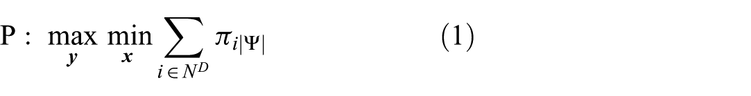
As indicated within the objective function (1), the defender and attacker, respectively, seek to maximize and minimize the cumulative time to collectively service the demands. Revisiting the motivating military application, the cumulative service time for each demand node is an appropriate performance metric of interest because the players are focused on the time at which a target is destroyed. For the civil application context, this timing indicates the full provision of needs to a demand, i.e., what matters to the citizens who pay taxes and vote for the elected officials who manage emergency relief systems.

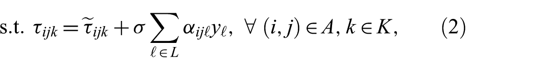
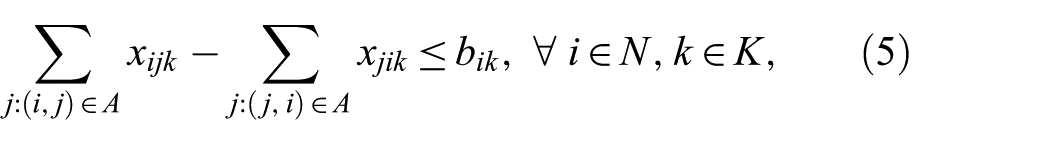
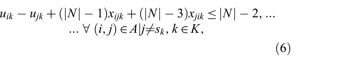
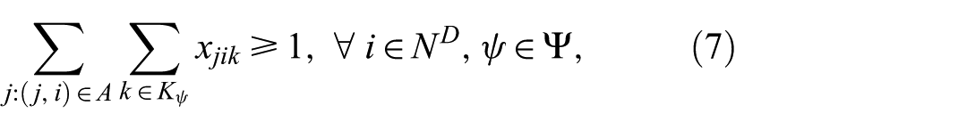
Constraint (2) computes the arc travel times $τ_{ijk}$ as affected by the defender’s interdiction strategy. The adopted representation is additive and linear. Alternative representations are possible, e.g., wherein disruptive actions impose a percentage increase to travel times, and may be embraced as appropriate for the applied problem of interest. Constraint (3) bounds the number of disruptive actions to be equal to $η$ , and constraint (4) limits the $y_{ℓ}$ -variables to be non-negative and integer-valued, allowing more than one disruption at a given location.

For the attacker’s routing problem, constraint (5) enforces the conservation of flow for the movement of assets without requiring their return to respective origins. Constraint (6) applies a lifted variant of the MTZ subtour elimination constraints. Constraint (7) requires at least one asset $k$ of each type $ψ \in Ψ$ to visit each demand node $i \in N^{D}$ .

Constraints (8) and (9) calculate the time at which each asset visits nodes as it moves through the network. Within constraint (9), the term $ω τ_{ijk}$ allows assets to slow down to $1 / ω$ of their fastest speed for traversing an arc $(i, j)$ to coordinate sequential arrival times at demands. Such a slower arc-traversing speed may manifest as either a constant or variable speed, the latter of which can include dwell time at any point along the arc. In either case, an asset’s minimum feasible speed must inform a selection of $ω$ (e.g. so a fixed-wing aircraft does not stall and crash), and a practitioner may alternatively implement $ω_{k}$ , with $ω$ -values specific to each asset. When applied to instances, one may parameterize $M$ to be equal to the longest time required to visit every demand node. Alternatively, it suffices to set $M = \max_{k \in K} {\sum_{(i, j) \in A} 2 τ_{ijk}}$ . Constraint (10) requires $t_{ik} = 0$ if asset $k$ never visits node $i$ .

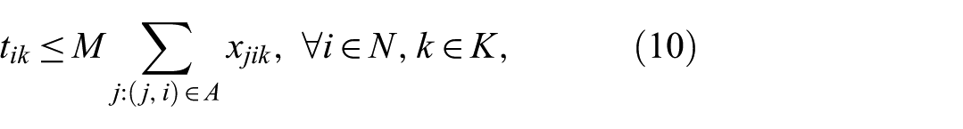
Constraint (11) bounds $π_{i ψ}$ -values below by the latest asset of type $k \in K_{ψ}$ to arrive at node $i \in N^{D}$ . For the motivating military application of interest, this constraint assumes an attacker would not route multiple assets of the same type through a common node to avoid presenting a defender with unnecessary opportunities to observe and engage attacker assets at a given location, e.g., to engage attacking assets directly. Additional testing not reported herein examined Special Ordered Set (SOS) Type 1 variables to allow a defender to instead determine which of multiple assets $k \in K_{ψ}$ of type $ψ$ that could pass through a demand node $i \in N^{D}$ “counted” toward bounding $π_{i ψ}$ , but doing so required an additional $| N^{D} | | K |$ binary variables and $| N^{D} | | Ψ |$ constraints that encumbered a formulation without observed benefit in preliminary testing. For each asset type, constraints s (12) and (13) collectively impose an upper bound on $ψ_{i ψ}$ to affix the visit to a node by the latest asset of type $k \in K_{ψ}$ . Constraint (14) ensures the visits by asset types do not violate an ordinal sequence, with simultaneous visits allowed. For each demand node, constraint (15) requires the sequence of visits by asset types to occur within a range of $δ$ units of time.

Finally, constraints (16)–(20) enforce the respective, appropriate restrictions on the decision variables.

As an aside, we note that Problem P has a convenient, alternative use. As formulated, it considers a defender seeking to delay an attacker via route-delaying interdictions at locations $ℓ \in L$ . Alternatively, consider those locations to be where an attacker may impose additional security measures to protect travel over nearby arcs $(i, j)$ , which would allow faster travel due to the enhanced security. For such a case, $σ < 0$ ; the attacker controls the $y_{ℓ}$ -variables; the objective is a strict minimization problem, and the mixed-integer linear program may be solved directly with a commercial solver. Beyond the scope of this research, one may also modify Problem P as a competitive location and routing model, wherein a defender imposes a set of delaying actions, and an attacker both imposes a set of security measures and routes the assets.

2.2. Solution methodology

It is of merit to analyze the formulation of Problem P to identify an appropriate solution methodology. Bilevel programming problems are $NP$ -hard.²⁷ As a (notably) more complicated variant of a VRP formulation, the lower-level problem embedded within Problem P is also $NP$ -hard.⁴⁸ Thus, the overall complexity of Problem P is $Σ_{2}^{p}$ -hard.⁴⁹

The $NP$ -hard nature of bilevel programs does not preclude the existence of transformations to yield more readily solvable, equivalent formulations. For a bilevel program with different upper-level and lower-level objective functions, replacing the lower-level problem with its Karush–Kuhn–Tucker optimality conditions⁷ yields a single-level, nonlinear program that can be solved directly via a commercial solver, subject to certain convexity-related constraint qualifications on the lower-level problem in Problem P. For a bilevel program like Problem P wherein there is a single objective function in tension (i.e. a zero-sum Stackelberg game), one may take the dual of the lower-level (a.k.a., inner) problem^9,50,51 to attain a single-level nonlinear program, again subject to certain convexity conditions on the lower-level problem.

Although the lower-level formulation in Problem P has binary-valued $x_{ijk}$ -variables, the latter of the aforementioned techniques is viable if an integer-valued solution is optimal when these (binary) integer restrictions are relaxed, i.e., if the lower-level formulation’s system of constraints exhibits total unimodularity.⁵² Unfortunately, this requirement does not hold, due to constraints (8) and (9). These VRP-style constraints encourage decimal-valued solutions in $x$ by splitting flows to attain artificially lower node arrival times $t$ and, in turn, artificially lower demand service times $π$ in the objective function. Thus, we must solve the bilevel program rather than a relaxation-induced, single-level transformation.

For a given defender solution $y$ , one may solve the ( $NP$ -hard) lower-level problem directly via a commercial solver. As such, one may solve Problem P by searching the upper-level feasible region and, for each solution $y$ , identify a corresponding, optimal solution to the lower-level problem, i.e., a best response by the defender. Such a search procedure is akin to searching the first stage in a two-stage, extensive form game tree, where an optimal solution to Problem P corresponds to a subperfect Nash equilibrium.

An exhaustive enumeration of the upper-level feasible region is unwise. For $η$ disruptive actions and $| L |$ possible locations where they can occur, a defender has $(\binom{η + | L | - 1}{| L | - 1})$ feasible solutions. Given the integer-restricted nature of the decision variables $y$ , it is possible to search the upper-level feasible region via a branch-and-bound approach,⁵³ but the exhaustive nature of such a method portends computational tractability issues, given the $NP$ -hard nature of the lower-level problem. Thus, it is of interest to rapidly identify high-quality solutions to the upper-level problem via an effective construction heuristic and seek to improve upon them via an efficient metaheuristic. The remainder of this section proposes a conceptually motivated construction heuristic to be applied in isolation or in combination with other metaheuristics, which Section 3 will evaluate via computational testing.

We propose three solution methods to search the upper-level feasible region to identify high-quality solutions with relative computational efficiency. As Table 1 indicates, these methods, respectively, consist of a greedy construction heuristic (GCH); GCH followed by simulated annealing (SA); and GCH followed by an enhanced variant of simulated annealing (eSA).

Table 1.

Solution methods examined.

Name	Construction heuristic	Improvement metaheuristic
GCH	Greedy	–
SA	Greedy	Simulated annealing (SA)
eSA	Greedy	Enhanced SA

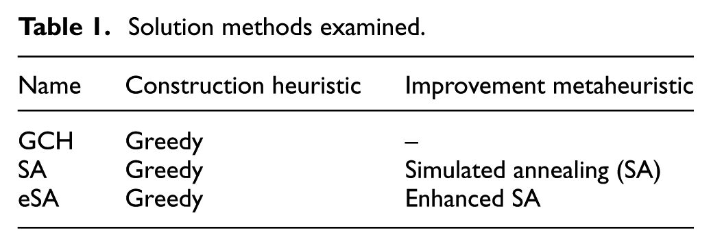
Whereas the first solution method entails only the identification of a feasible solution using GCH, the second solution method subsequently applies a simulated annealing metaheuristic.⁵⁴ We selected simulated annealing as a baseline metaheuristic because GCH provides a single solution upon which to improve. In contrast, population-based metaheuristics (e.g. genetic algorithms,⁵⁵ particle swarm optimization,⁵⁶ and ant colony optimization)⁵⁷ require more initial candidate solutions, and their generation would require the embrace of deliberately worse construction heuristics or random interdiction strategies, neither of which has conceptual appeal. Other single-solution metaheuristics are certainly available (e.g. Tabu search⁵⁸ and GRASP)⁵⁹, and a consideration of their mechanisms informs the third solution method. Subsequent discussion details the components of each solution method and their implementation.

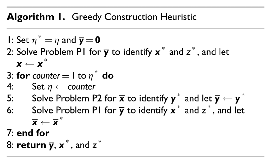
2.2.1. Greedy construction heuristic

GCH identifies a conceptually effective, feasible solution to Problem P. Whereas greedy heuristics entail no assurance of identifying an optimal solution, a logical series of choices when constructing a feasible solution will often yield a good solution. Given $η$ disruptive actions allowed, GCH identifies a solution by iteratively identifying each subsequent disruptive action location $ℓ \in L$ by solving the lower-level problem $(η + 1)$ times.

Define Problem P1 as the lower-level problem within Problem P, which seeks to minimize the objective function subject to constraints (5)–(20), given a feasible interdiction strategy $\bar{y}$ . Solving P1 identifies an optimal asset-routing solution.

Define Problem P2 as Problem P with the goal of only maximizing the objective function, given both a fixed, partial attacker routing solution $\bar{x}$ and a fixed, partial defender solution $\bar{y}$ where $\sum_{ℓ \in L} {\bar{y}}_{ℓ} = (η - 1)$ , and with the additional constraint $y_{ℓ} \geq {\bar{y}}_{ℓ}, \forall ℓ \in L$ . Solving Problem P2 identifies the best location for the $η^{th}$ disruptive action, given $(η - 1)$ such actions have been identified and are fixed.

Leveraging these definitions, Algorithm 1 presents GCH. Line 1 initializes the total number of disruptive actions $η^{*}$ and a null interdiction solution $\bar{y}$ . Line 2 identifies an optimal routing solution $\bar{x}$ in the absence of interdiction and updates the current routing solution. Within Lines 3–7, GCH iteratively identifies the location of the disruptive actions. For each such action, Line 4 increments the number of actions $η$ by 1; Line 5 identifies the location of the additional action within the updated interdiction strategy $\bar{y}$ ; and Line 6 identifies the best asset-routing response $\bar{x}$ . Upon termination, Line 8 returns the interdiction strategy $\bar{y}$ , feasible to Problem P with the objective function value $z^{*}$ .

Algorithm 1. Greedy Construction Heuristic
1: Set $η^{} = η$ and $\bar{y} = 0$ 2: Solve Problem P1 for $\bar{y}$ to identify $x^{}$ and $z^{}$ , and let $\bar{x} \leftarrow x^{}$ 3: for $counter = 1 to η^{}$ do 4: Set $η \leftarrow counter$ 5: Solve Problem P2 for $\bar{x}$ to identify $y^{}$ and let $\bar{y} \leftarrow y^{}$ 6: Solve Problem P1 for $\bar{y}$ to identify $x^{}$ and $z^{}$ , and let $\bar{x} \leftarrow {\bar{x}}^{}$ 7: end for 8: return $\bar{y}$ , $x^{}$ , and $z^{}$

Algorithm 1. Greedy Construction Heuristic

1: Set

η^{*} = η

and

\bar{y} = 0

2: Solve Problem P1 for

\bar{y}

to identify

x^{*}

and

z^{*}

, and let

\bar{x} \leftarrow x^{*}

3: for

counter = 1 to η^{*}

do
4: Set

η \leftarrow counter

5: Solve Problem P2 for

\bar{x}

to identify

y^{*}

and let

\bar{y} \leftarrow y^{*}

6: Solve Problem P1 for

\bar{y}

to identify

x^{*}

and

z^{*}

, and let

\bar{x} \leftarrow {\bar{x}}^{*}

7: end for
8: return

\bar{y}

x^{*}

, and

z^{*}

2.2.2. Simulated annealing metaheuristic

Originally developed by Kirkpatrick et al.,⁵⁴ SA is a useful improvement metaheuristic for vehicle routing problems (e.g. Osman,⁶⁰ Van Breedam,⁶¹ Chiang and Russell,⁶² Vincent et al.,⁶³ and Prihodko et al.⁶⁴) and, more specifically, for VRPs with fixed time windows (e.g. Laporte et al.⁶⁵ and Mohammadi et al.⁶⁶). Other interdiction models have explored the use of SA to achieve near optimal solutions for large scale models (e.g. Janjarassuk and Nakrachata-Amon,⁶⁷ Parsafard and Li⁶⁸). The SA framework has also proven effective at finding solutions to the latency location routing problem,⁶⁹ which minimizes the sum of arrival times to service demands.

Whereas a hill-climbing algorithm or descent method seeks only to improve solutions, the SA metaheuristic allows a move within a feasible region from a current solution to a solution with a worse objective function value. The goal of this allowance is to avoid becoming trapped in a local optimum that would otherwise preclude a broader search of the feasible region, thereby improving the likelihood of identifying a global optimum. Such a wariness of converging to a local-but-not-global optimum is warranted for nonconvex optimization problems, including mixed-integer linear programming problems like Problem P.

Each iteration of a conventional implementation of SA functions as follows. Given a feasible solution and a defined neighborhood of solutions, identify and evaluate a candidate solution in the neighborhood. If the candidate solution is feasible and has an improved objective function value, accept it as the new solution with certainty; otherwise, accept it as the new solution with some probability $p$ . As SA proceeds, the metaheuristic deliberately reduces $p$ , typically fast initially and then slower. Much like the malleability of a metal that is cooled via an annealing process, the willingness of SA to adopt a worse candidate solution reduces over time (i.e. iterations), eventually hardening (i.e. converging) to the behavior of a hill-climbing algorithm or descent method. SA typically terminates after a fixed, user-defined number of iterations or when a temperature parameter $T$ used to calculate $p$ decreases below a predetermined value $T^{*}$ .⁵ Affecting its performance notably, an SA implementation has two important characteristics: (1) its definition of a neighborhood and (2) a probability function with associated parameters to define the probability $p$ .

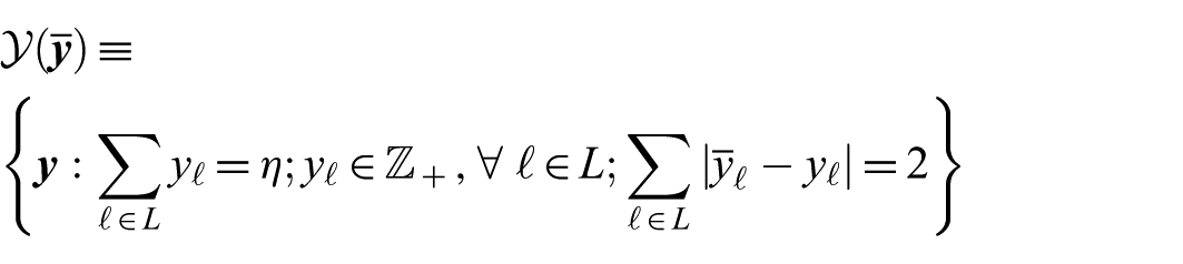
SA Neighborhood Definition. Given a feasible interdiction strategy $\bar{y}$ for Problem P, we define the neighborhood to be

\begin{matrix} Y (\bar{y}) \equiv \\ {y : \sum_{ℓ \in L} y_{ℓ} = η; y_{ℓ} \in Z_{+}, \forall ℓ \in L; \sum_{ℓ \in L} | {\bar{y}}_{ℓ} - y_{ℓ} | = 2} \end{matrix}

In practice, one can identify a candidate solution $y^{'} \in Y (\bar{y})$ by selecting a single location $\tilde{ℓ}$ in the current solution, having $y_{\tilde{ℓ}} \geq 1$ and moving a disruptive action from that location to any other location $ℓ^{'} \in L ∖ {\tilde{ℓ}}$ . Our implementation of SA identifies a candidate solution $y^{'}$ in this manner, selecting the location $\tilde{ℓ}$ from a discrete uniform distribution over all disruptive action locations and the new location for a disruptive action via a discrete uniform distribution over $ℓ \in L ∖ {\tilde{ℓ}}$ .

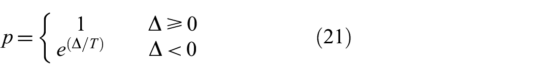
Solving P1 for the candidate solution $y^{'}$ yields an optimal objective function value $z^{'}$ . Denoting the current solution’s optimal objective function value for P1 is $\bar{z}$ , the relative (%) objective function value increase is $Δ = (z^{'} - \bar{z}) / \bar{z}$ .

SA Probability Function. The probability function defined in Equation (21) computes the likelihood $p$ with which SA accepts a candidate solution $y^{'}$ within a given iteration, as a function of both $Δ$ and a declining temperature parameter, $T$ . As indicated by the conditions on $Δ$ , our SA implementation accepts any candidate solution that is not worse than the current solution with certainty, and it accepts a worse solution with probability $p$ , declining exponentially on $(Δ / T)$ for negative values of $Δ$ .

p = {\begin{matrix} 1 & Δ \geq 0 \\ e^{(Δ / T)} & Δ < 0 \end{matrix}

(21)

Of note, $T$ is not a fixed parameter; initialized with a temperature $T = T_{0}$ , it decreases with each iteration to affect the annealing process for any fixed $Δ < 0$ . Many functional forms (e.g. linear and geometric) are available to update the temperature $T$ . Based upon initial computational testing for instances of Problem P, we adopted the temperature update function given by Equation (22) for a user-determined parameter $β > 0$ .

T \leftarrow \frac{T}{1 + β T}

(22)

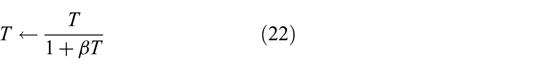
Defining the temperature threshold and maximum iteration count used for alternative SA termination criteria as $T^{*}$ and ${iter}_{\max}$ , respectively, Algorithm 2 presents our implementation of the SA metaheuristic to solve an instance of Problem P, returning the best identified interdiction strategy $y^{*}$ , the corresponding best routing response $x^{*}$ , and the resulting objective function value $z^{*}$ .

Algorithm 2. SA Implementation
1: Given $\bar{y}$ feasible to Problem P1, $T_{0}$ , $T^{}$ , and ${iter}_{\max}$ 2: Solve P1 for $\bar{y}$ to identify $\bar{x}$ and $\bar{z}$ 3: Let $y^{} \leftarrow \bar{y}$ , $x^{} \leftarrow \bar{x}$ , $z^{} \leftarrow \bar{z}$ , and $T \leftarrow T_{0}$ 4: for $iter = 1 to {iter}_{\max}$ do 5: Update $T$ via Equation 22 6: Identify a candidate solution $y^{'} \in Y (\bar{y})$ 7: Solve P1 for $y^{'}$ to identify $x^{'}$ and $z^{'}$ , and compute $Δ$ 8: With probability $p$ via Equation (21), let $\bar{y} \leftarrow y^{'}$ , $\bar{x} \leftarrow x^{'}$ , and $\bar{z} \leftarrow z^{'}$ 9: if $\bar{z} > z^{}$ then 10: Let $y^{} \leftarrow \bar{y}$ , $x^{} \leftarrow \bar{x}$ , $z^{} \leftarrow \bar{z}$ 11: end if 12: if $T < T^{}$ then 13: break 14: end if 15: end for 16: return $y^{}$ , $x^{}$ , and $z^{}$

Algorithm 2. SA Implementation

1: Given

\bar{y}

feasible to Problem P1,

T_{0}

T^{*}

, and

{iter}_{\max}

2: Solve P1 for

\bar{y}

to identify

\bar{x}

and

\bar{z}

3: Let

y^{*} \leftarrow \bar{y}

x^{*} \leftarrow \bar{x}

z^{*} \leftarrow \bar{z}

, and

T \leftarrow T_{0}

4: for

iter = 1 to {iter}_{\max}

do
5: Update

T

via Equation 22
6: Identify a candidate solution

y^{'} \in Y (\bar{y})

7: Solve P1 for

y^{'}

to identify

x^{'}

and

z^{'}

, and compute

Δ

8: With probability

p

via Equation (21), let

\bar{y} \leftarrow y^{'}

\bar{x} \leftarrow x^{'}

, and

\bar{z} \leftarrow z^{'}

9: if

\bar{z} > z^{*}

then
10: Let

y^{*} \leftarrow \bar{y}

x^{*} \leftarrow \bar{x}

z^{*} \leftarrow \bar{z}

11: end if
12: if

T < T^{*}

then
13: break
14: end if
15: end for
16: return

y^{*}

x^{*}

, and

z^{*}

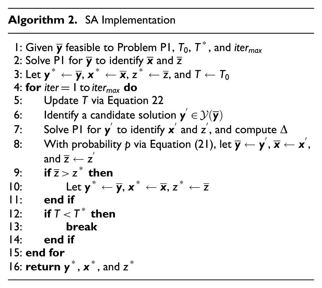
Within Algorithm 2, Line 1 recognizes the initial feasible solution, the initial temperature parameter, and the two alternative termination criteria. Line 2 identifies the best routing response for the interdiction strategy and the corresponding objective function value. Given an initial solution identified via GCH, Line 2 is not necessary, but we retain it to represent SA for alternative means to identify an initial feasible solution (e.g. a randomly generated interdiction strategy). Line 3 initializes the incumbent solutions and cooling temperature. Within Lines 4–15, SA identifies and evaluates at most ${iter}_{\max}$ candidate solutions. Line 5 updates the cooling temperature. Line 6 identifies a candidate solution, and Line 7 evaluates it. Line 8 determines whether to accept the candidate solution as the current solution, and Lines 9–11 update the incumbent solution if appropriate. An iteration concludes by comparing if $T$ is lower than the threshold $T^{*}$ , and, if so, Lines 12–14 terminate the for loop. Otherwise, iterations continue until $iter = {iter}_{\max}$ , after which the procedure concludes in Line 16 with the best identified interdiction strategy, routing response, and objective function value.

2.2.3. Enhanced simulated annealing metaheuristic

Within Algorithm 2, Line 6 incurs a notable computational expense. As previously discussed, Problem P1 is $NP$ -hard. The enhanced simulated annealing (eSA) metaheuristic seeks to reduce the number of times it solves Problem P1 without a productive exploration of the upper-level feasible region. More specifically, SA exhibits two inefficiencies, as implemented in Algorithm 2. First, a candidate solution $y^{'}$ may have been previously explored. Second, the generation of a candidate solution $y^{'}$ from a current solution $\bar{y}$ may remove an effective disruptive action while adding an ineffective action elsewhere. The eSA metaheuristic addresses these computational inefficiencies via two mechanisms: (1) a tabu list and (2) an alternative method to generate candidate solutions.

Borrowing from the Tabu Search metaheuristic,⁵⁸ eSA maintains a bounded tabu list of the most recently examined interdiction solutions. If a candidate solution $y^{'}$ is on the list, eSA identifies an alternative candidate solution to evaluate. Other interdiction research (e.g. Michalopoulos et al.⁷⁰ and Aksen and Aras⁷¹) has directly applied Tabu Search, so there is precedent for a tabu list for reducing computational effort when solving a bilevel program.

With regard to generating a candidate solution in Line 6 of Algorithm 2, eSA discards the randomized mechanisms for moving a disruptive action to a new location, as discussed in Section 2.2.2. It instead embraces a conceptually greedy approach, seeking to move a (perceived) least effective disruptive action to a location where it would be most effective. Given a solution $\bar{y}$ , only $\tilde{ℓ}$ and $ℓ^{'}$ are necessary to define the candidate solution $y^{'}$ . Algorithm 3 defines the eSA process to identify $(\tilde{ℓ}, ℓ^{'})$ and, in turn, $y^{'}$ .

Algorithm 3. eSA Identification of $y^{'}$
1: Given a tabu list $T$ , an interdiction strategy $\bar{y}$ , and $x^{}$ as the corresponding solution to Problem P1 2: Define R1 as a list of current disruptive action locations $\tilde{ℓ}$ , sorted in ascending order on $\sum_{(i, j) \in A} \sum_{k \in K} α_{ij \tilde{ℓ}} x_{ijk}^{}$ 3: Define ${R 2}_{\tilde{ℓ}}$ as a list of potential disruptive action locations $ℓ^{'} \in L ∖ {\tilde{ℓ}}$ , sorted in descending order on strictly positive values of $\sum_{(i, j) \in A} \sum_{k \in K} α_{ij ℓ^{'}} x_{ijk}^{*}$ 4: for $\tilde{ℓ} \in$ R1 do 5: for $ℓ^{'} \in$ ${R 2}_{\tilde{ℓ}}$ do 6: if $y^{'} \notin T$ then 7: return $y^{'}$ 8: end if 9: end for 10: end for

Algorithm 3. eSA Identification of

y^{'}

1: Given a tabu list

T

, an interdiction strategy

\bar{y}

, and

x^{*}

as the corresponding solution to Problem P1
2: Define R1 as a list of current disruptive action locations

\tilde{ℓ}

, sorted in ascending order on

\sum_{(i, j) \in A} \sum_{k \in K} α_{ij \tilde{ℓ}} x_{ijk}^{*}

3: Define

{R 2}_{\tilde{ℓ}}

as a list of potential disruptive action locations

ℓ^{'} \in L ∖ {\tilde{ℓ}}

, sorted in descending order on strictly positive values of

\sum_{(i, j) \in A} \sum_{k \in K} α_{ij ℓ^{'}} x_{ijk}^{*}

4: for

\tilde{ℓ} \in

R1 do
5: for

ℓ^{'} \in

{R 2}_{\tilde{ℓ}}

do
6: if

y^{'} \notin T

then
7: return

y^{'}

8: end if
9: end for
10: end for

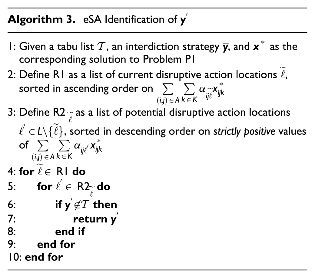
Within Algorithm 3, we seek to identify the pair of locations $(\tilde{ℓ}, ℓ^{'})$ that preemptively and, respectively, remove a disruptive action from the location affecting arcs least (currently) traveled by assets and move it to a location that will affect arcs most (currently) traveled by assets, such that the resulting solution $y^{'}$ is not on the tabu list. Line 1 recognizes the given information, and Lines 2 and 3 define the sorted lists R1 and ${R 2}_{\tilde{ℓ}}$ . If there is a tie when sorting any list, the respective ordering of indices having the same score is random. Lines 4–10 identify $y^{'}$ , wherein Lines 4 and 5 assume the iteration of elements in each list in the respective sorted orders. If Algorithm 3 terminates without identifying a $y^{'} \notin T$ , the eSA metaheuristic terminates.

Algorithm 3’s identification of $(\tilde{ℓ}, ℓ^{'})$ merits further discussion. Selecting $\tilde{ℓ}$ via R1 is an imperfect greedy approach. From an ideal perspective, it will be an ineffective disruptive action in the current interdiction solution. Alternatively, it may be a disruptive action that was so effective that the lower-level decision-maker avoided having agents traverse any nearby arcs. The possibility that $\tilde{ℓ}$ is poorly selected may provide an equivalent or better asset routing when a disruptive action is moved to $ℓ^{'}$ , resulting in $Δ < 0$ . As such, the sound conceptual motivation for Algorithm 3 implemented with eSA does not improve upon SA with certainty. Computational testing is necessary to assess their relative performances, as Section 3 examines.

3. Testing, results, and analysis

For a network $G (N, A)$ , we consider a regular hexagonal tessellation of a planar region, a discretization technique embraced in the literature for routing assets in a region not restricted to a road network, such as airspace (e.g. Lessin et al.,⁵¹ Yousefi and Donohue,⁷² and Lunday et al.⁷³). In addition, a hexagonal grid provides benefit of well-defined areas for disruptive actions, i.e., $ℓ \in L$ as center of a hexagon, wherein a disruptive action (i.e. where $y_{ℓ} \geq 1$ ) slows travel across all arcs bordering the hexagon.

3.1. Illustrative example

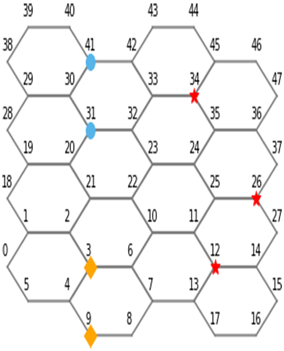
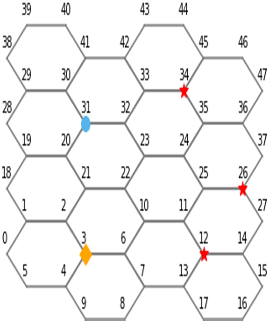
For the illustrative example, Figure 1 presents the hexagonal mesh with 16 regular hexagons (i.e. $| L | = 16$ ). Depicted on the network are $K = {1, 2}$ assets and $Ψ = {1, 2}$ asset types, with $K_{1} = {1}$ and $K_{2} = {2}$ having respective origins indicated by the blue circle at Node 31 and the orange diamond at Node 3. Red stars indicate the set of demand points $N^{D} = {12, 26, 34}$ . Asset Types 1 and 2 have different minimum travel times of $(τ_{ij 1}, τ_{ij 2}) = (1, 0.8)$ , $\forall (i, j) \in A$ , and the maximum range of time between when assets of Types 1 and 2 must, respectively, service a demand is $δ = 5$ .

Figure 1.

Illustrative example: Hexagonal mesh, initial asset locations, and demand node locations.

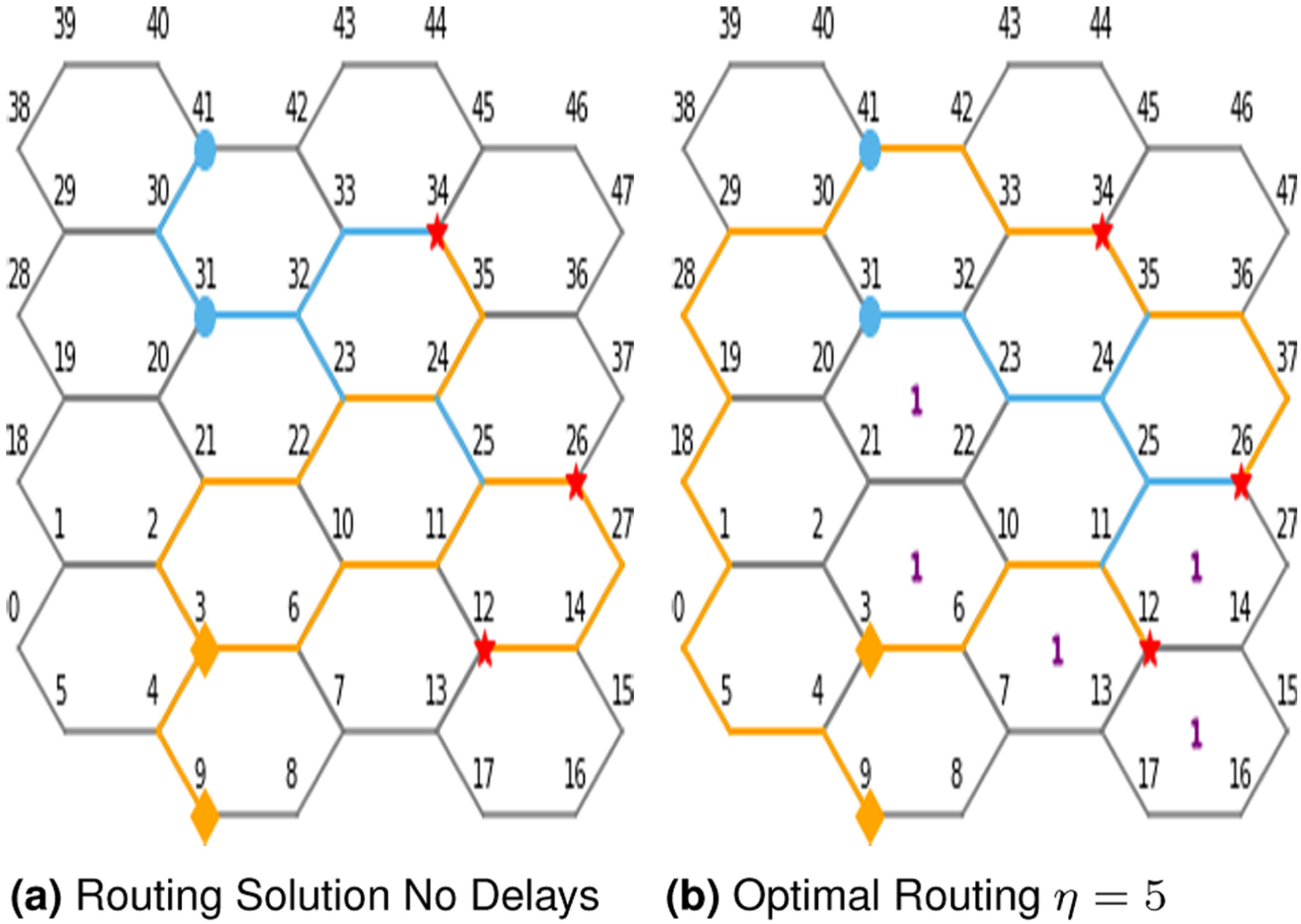
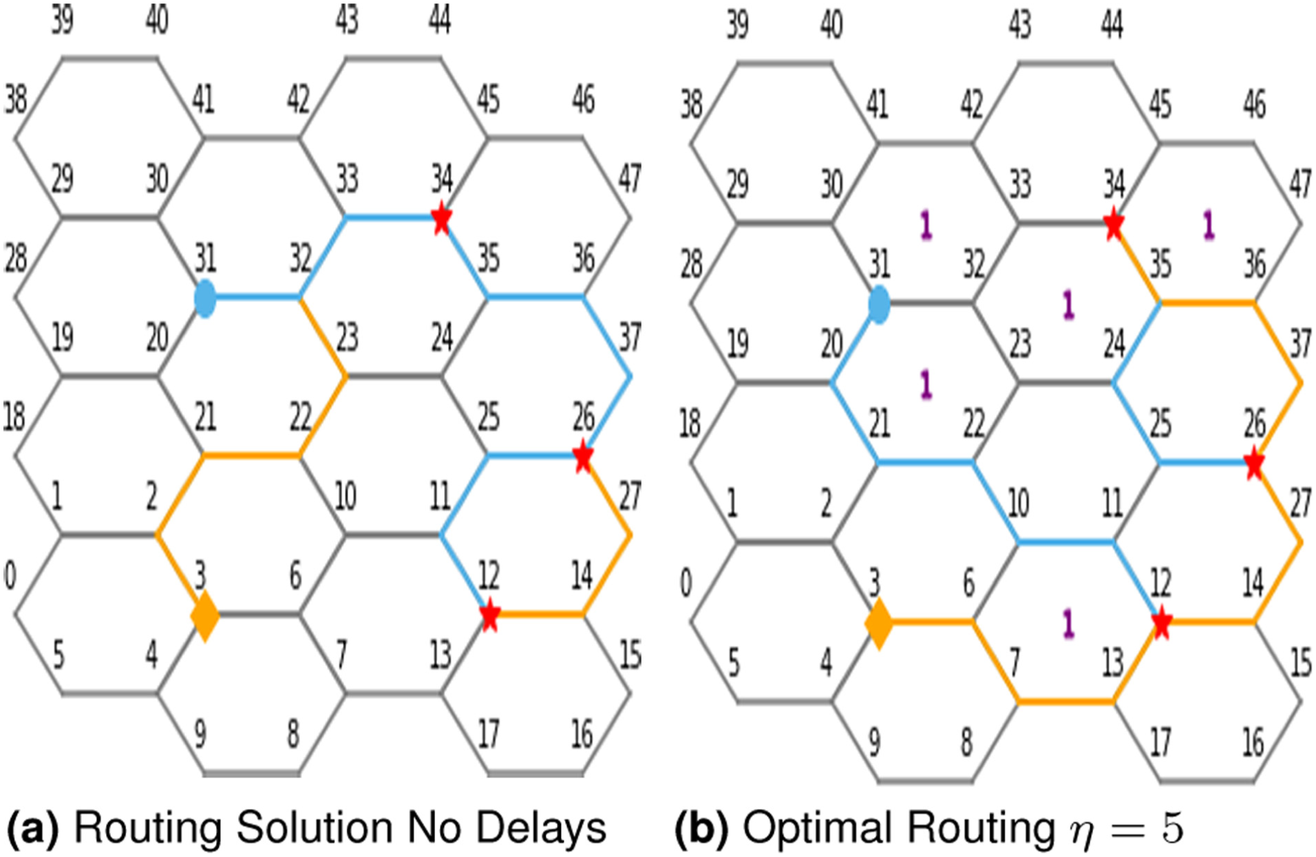
Figure 2(a) illustrates an optimal routing of the assets to service demands in the absence of delaying actions implemented by the defender (i.e. $η = 0$ ), corresponding to an objective function value of 25.6. Figure 2(b) presents the delaying actions found via GCH with $η = 5$ and the corresponding optimal asset-routing solution for the lower-level problem. The delaying actions increase travel time on the affected arcs by $σ = 1.5$ time units. Figure 2(b) depicts numerals (e.g. 1) in the center of hexagons where $y_{ℓ} = 1$ , indicating the number of delaying actions at the center of selected hexagons, in turn increasing travel times on the bordering arcs. With the $η = 5$ disruptions depicted, the optimal asset-routing solution has a minimal objective function value of 55.

Figure 2.

Example model execution. (a) Routing solution with no delays. (b) Optimal routing $η = 5$ .

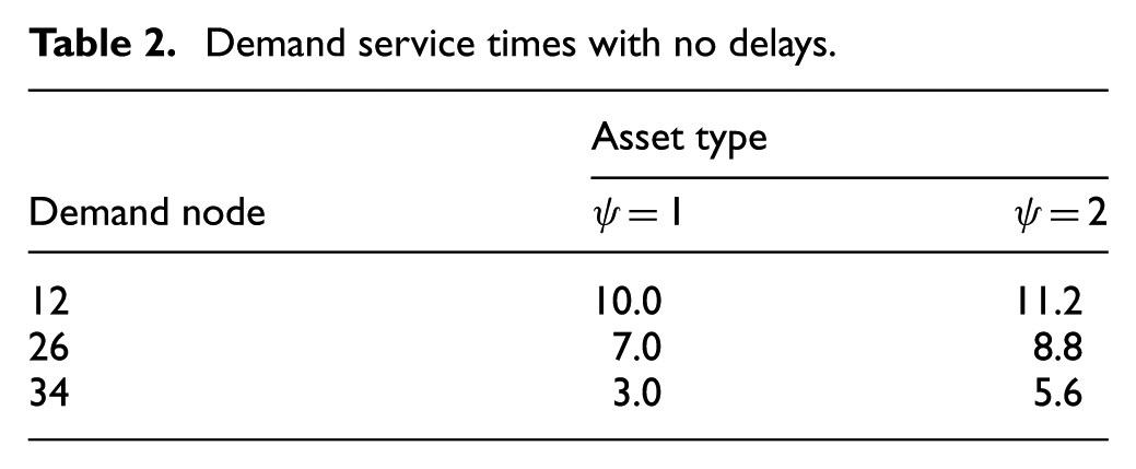
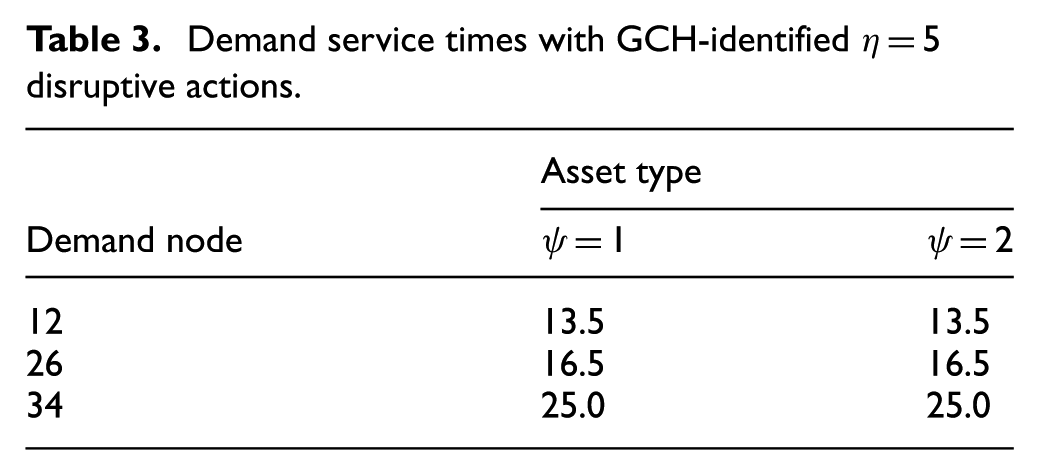
Accompanying the visual depictions in Figure 2(a) and (b), Tables 2 and 3 report the $π_{i}$ -values resulting from the arrival times of asset types $ψ = 1$ (i.e. asset $k = 1$ ) and $ψ = 2$ (i.e. asset $k = 2$ ) at each of the demand nodes. Examining the rightmost columns, the GCH-identified delaying actions increase the cumulative service time by 29.4, resulting from delaying the servicing of Nodes 12, 26, and 34, respectively, by 2.3, 7.7, and 24.4 time units. Also compelling, the disruptive actions change the optimal routes of the assets, reverse the order in which the demands are serviced, and compel simultaneous servicing of demands by both assets.

Table 2.

Demand service times with no delays.

	Asset type
Demand node	$ψ = 1$	$ψ = 2$
12	10.0	11.2
26	7.0	8.8
34	3.0	5.6

Table 3.

Demand service times with GCH-identified $η = 5$ disruptive actions.

	Asset type
Demand node	$ψ = 1$	$ψ = 2$
12	13.5	13.5
26	16.5	16.5
34	25.0	25.0

As an aside, there do exist alternative optima for the asset routing. The two paths traversing from Node 26 to Node 35 (i.e. $26 - 25 - 24 - 35$ and $26 - 37 - 36 - 35$ ) in Figure 2(b) are equivalent. Such a characteristic is more likely to exist in optimal asset-routing solutions for instances having common arc traversal times and a graph induced via a regular tessellation of a region, which collectively contribute to problem symmetry. Given this observation, specialized techniques such as orbital branching⁷⁴ may reduce the required computational effort to solve the lower-level problem, although the exploration of such techniques is beyond the scope of this study.

3.2. Parameter exploration

To evaluate the potential of both SA and eSA to improve upon the GCH-identified solution, testing considered alternative numbers of delaying strategies ( $η$ ), initial temperature values ( $T_{0}$ ), and the cooling rate parameter ( $β$ ) used in the temperature update function, as discussed in Section 2.2.2. Table 4 displays the parameter values explored herein.

Table 4.

Values to explore.

Factor	Values explored
Number delaying actions, $η$	$3, 4, 5, 6$
Initial temperature, $T_{0}$	$1, 5$
Cooling rate parameter, $β$	$0.01, 0.1$

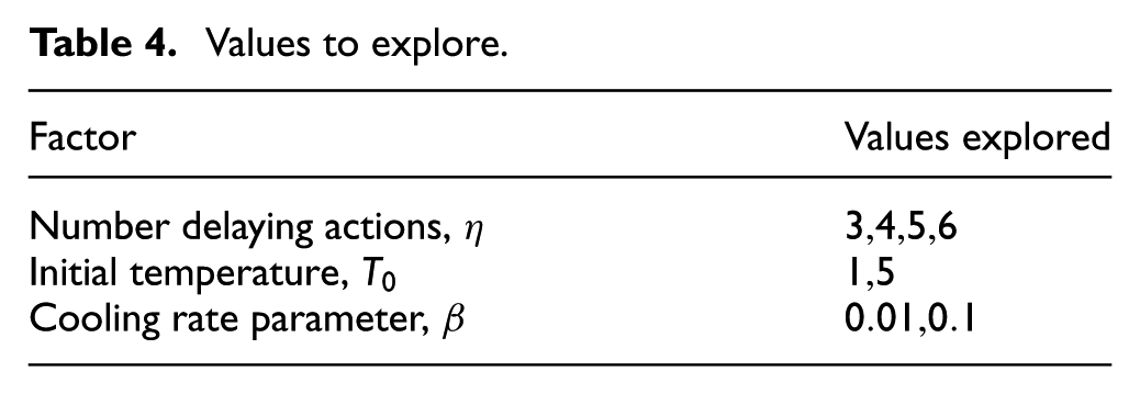
For the baseline instance depicted in Figure 2(a), testing examined both SA and eSA with a combination of the parameters in Table 4, initializing them with a GCH-identified solution having the same $η$ -value and using a common random seed. The effect of high and low values of both $T_{0}$ and $β$ explored the respective impacts of the temperature update function and the probability of accepting a candidate solution that will not yield an immediate improvement. Both SA and eSA terminated after 45 iterations or when the annealing temperature dropped below 0.05, whichever came first. All testing was performed on an Intel(R) Core(TM) i7-10875 H CPU @2.30 GHz with 128 GB of RAM on a 64-bit operating system, and using Python (Version 3.9.7) with the GurobyPi package to invoke the commercial solver Gurobi (Version 9.5.1). When solving the lower-level problems using Gurobi, alternative termination criteria were 1800 s (i.e. 30 min) of computational effort and an identified 0.0005% relative optimality gap.

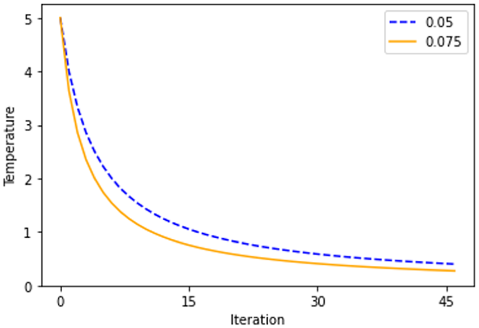
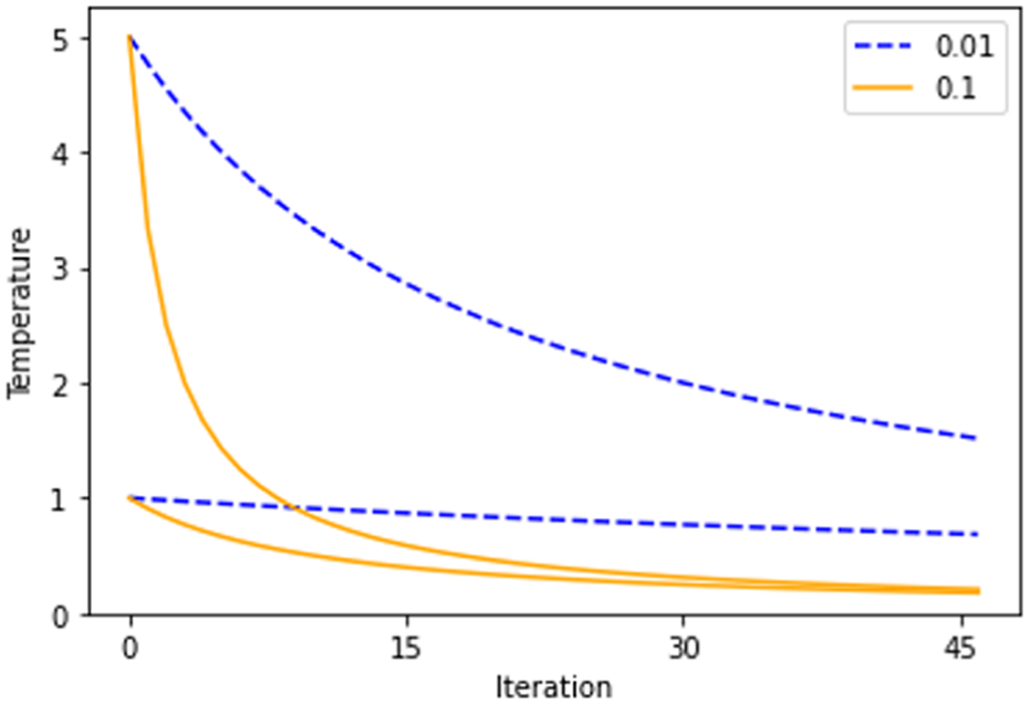
Figure 3 depicts four temperature update functions over the respective $(T_{0}, β)$ -combinations over 45 iterations. It depicts faster initial decreases in temperature for larger values of $β$ or $T_{0}$ . Of note, the combination of $(T_{0}, β) =$ (5,0.01) never exhibits a temperature below 1, even after 45 iterations.

Figure 3.

Annealing temperature as a function of $T_{0}$ and $β$ .

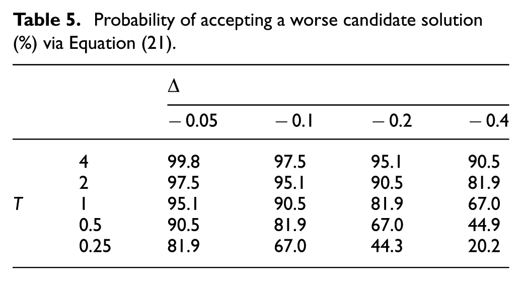
If a candidate solution improves the currently accepted solution, both the SA and eSA algorithms will accept it with certainty; otherwise, the probability of acceptance is determined by current temperature, $T$ , and the change between the current solution and candidate solution, $Δ$ . Table 5 presents the probability (%) of accepting a worse candidate solution over a sample of $(T, Δ)$ -value combinations. When $T > 1$ , the probability of accepting the candidate solution is greater than 0.5, even if the solution is notably worse. When $T < 1$ , acceptance of the candidate solution depends on a lower magnitude for $Δ$ . This leads to an understanding that a high $T_{0}$ -value paired with a low $β$ -value will more likely accept worsening candidate solutions, regardless of how much worse they are. Conversely, a low $T_{0}$ paired with a high $β$ -value are less likely to accept a worse candidate solution, even if the magnitude of its $Δ$ -value is small.

Table 5.

Probability of accepting a worse candidate solution (%) via Equation (21).

		$Δ$
		−0.05	−0.1	−0.2	−0.4
	4	99.8	97.5	95.1	90.5
	2	97.5	95.1	90.5	81.9
$T$	1	95.1	90.5	81.9	67.0
	0.5	90.5	81.9	67.0	44.9
	0.25	81.9	67.0	44.3	20.2

3.3. Comparative testing of solution methods

Table 6 reports the objective function value attained via GCH for each of the $η$ -values explored. Because the GCH algorithm iteratively adds a delaying strategy to the solution, the objective function value strictly increases with $η$ and does so at a reasonably steady rate. The remainder of this section explores the relative performances of SA and eSA. The GCH-identified $y_{ℓ}$ -values initialize both the SA and eSA algorithms.

Table 6.

Objective function values for solutions identified via the greedy construction heuristic.

$η$	Objective
3	42.7
4	47.0
5	55.0
6	62.2

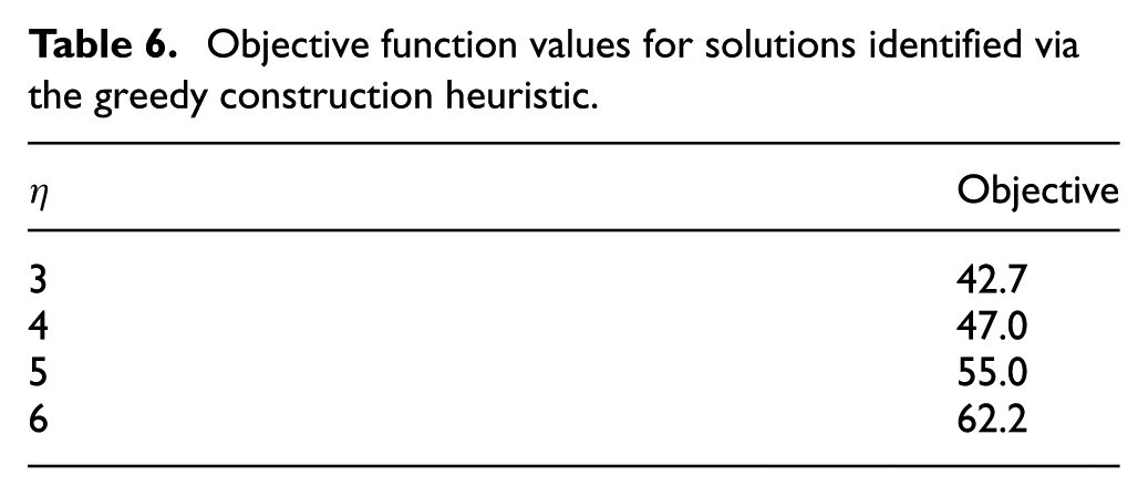
Table 7 presents the best objective function value found after 45 iterations of SA and eSA for each combination $η$ , $T_{0}$ , and $β$ from Table 4. SA identified an improved solution over GCH for 12 of the 16 instances. It failed to do so only when $T_{0} = 1$ , three times of which occurred with $β = 0.01$ , indicating the relatively poor performance of that parametric combination for SA. This outcome is likely due to the lower probability of accepting a worse candidate solution (i.e. getting stuck in a local-but-not-global optimal solution). In contrast, eSA improved upon the GCH solution at each $η$ -value and for every combination of $(T_{0}, β)$ -parameters.

Table 7.

Best objective function value after 45 iterations for the SA and eSA algorithms.

		$η = 3$		$η = 4$		$η = 5$		$η = 6$
$T_{0}$	$β$	SA	eSA	SA	eSA	SA	eSA	SA	eSA
1	0.01	40.8	48.1	49.7	54.1	55.0	61.6	61.0	69.4
1	0.10	48.1	48.1	49.7	54.1	62.5	61.6	61.0	69.4
5	0.01	46.8	48.1	49.7	55.0	55.0	61.6	69.0	70.6
5	0.10	48.1	48.1	49.7	54.1	55.0	61.6	69.0	67.6

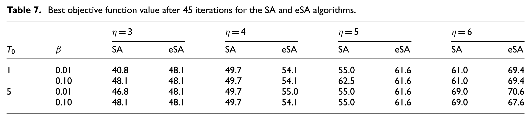
Whereas a higher initial temperature portends better outcomes, the effect of $β$ on the best identified objective function value is more nuanced. Higher $β$ -values performed the same or better when $T_{0} = 1$ , and lower $β$ -values more often did better when $T_{0} = 5$ , albeit not universally (i.e. SA did better with $(T_{0}, β) = (5, 0.10)$ than $(5, 0.01)$ with $η = 3$ ). Broader conclusions from the results in Table 7 are elusive, and Section 3.4 reports the results of additional testing specific to the effect of alternative $β$ -values.

Overall, these results compel an examination of whether the annealing aspect of the SA and eSA algorithms is effective. That is, for these instances, would SA or eSA perform better by either never accepting a worse candidate solution (i.e. $p = 0$ ) or always accepting it (i.e. $p = 1$ )? Table 8 reports the objective function value of the solution, respectively, identified by SA and eSA for $p = 0, 1$ and $η = 3, 4, 5, 6$ .

Table 8.

Best objective function value after 45 iterations for the SA and eSA algorithms in the absence of annealing, i.e., with fixed probability $p$ of accepting a worse candidate solution.

	$η = 3$		$η = 4$		$η = 5$		$η = 6$
$p$	SA	eSA	SA	eSA	SA	eSA	SA	eSA
0	46.6	46.6	54.3	55.6	60.0	61.8	66.7	66.7
1	46.8	48.1	49.7	55.0	55.0	61.6	69.0	70.6

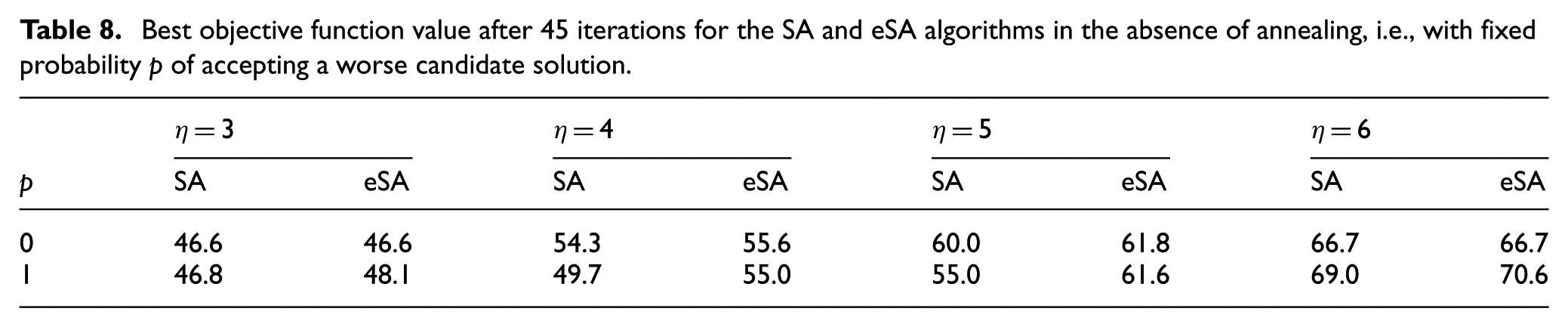
Within the results in Table 8, eSA performed as well or better than SA for each instance. However, neither never ( $p = 0$ ) nor always ( $p = 1$ ) accepting a worse candidate solution was a universally beneficial modification to either SA or eSA. Comparing the results with Table 7, eSA with $p = 0$ identified the best solution for $η = 4$ , and eSA with $p = 1$ did so for $η = 6$ . These results reinforce the merit of exploring alternative annealing schemes and parametric combinations.

For the testing reported in Tables 7 and 8, Table 9 presents the relative performance of eSA and SA regarding the objective function value and the required algorithmic runtime. More specifically, it tabulates the percentage of instances for which eSA performed as well as or better than SA. The first row aggregates the results over all combinations of $(T_{0}, β)$ -values and $p$ -values, and over all $η$ -values. The second and third rows partition the results by $η = 3, 4$ and $η = 5, 6$ , respectively.

Table 9.

Instances (%) for which eSA performed as well or better than SA.

$η$ -values	Objective function value	Runtime
3,4,5,6	91.7	66.7
3,4	100.0	75.0
5,6	83.3	58.3

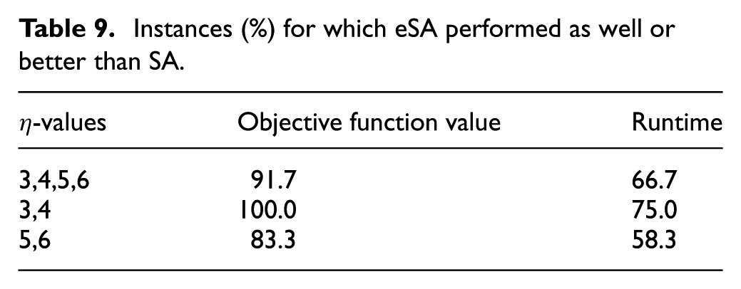
The eSA algorithm found equivalent or better solutions than SA for 91.7% of the instances of different $η$ -values and parametric combinations. There were two instances where SA found a strictly better solution, at $η = 5$ and $6$ , both when $β = 0.1$ . This result improved to 100% when restricted to smaller $η$ -values. The eSA had a faster runtime for more than half of the instances, which improved to 75% when considering only the lower $η$ -values.

In addition, testing examined the relative performance of eSA and SA over five different starting seeds for pseudorandom number generation. Not reported in detail here, testing found that eSA always found the same or better solutions than SA, and it found them more consistently; eSA found the same best solution across all random seeds explored, whereas SA identified a distinctly different best solution for each random seed.

3.4. Selected excursional analyses

Additional testing examined the effects of the different values of $β$ , as well as the quality of GCH-identified solutions and instance tractability for routing multiple assets of each type, and when routing a third asset type.

3.4.1. Sensitivity analysis for $β$ -values

Testing results in Section 3.3 indicated the merit of having higher $T_{0}$ -values to more likely accept worse candidate solutions. Affixing $T_{0} = 5$ , testing investigated the effects of $β$ -values of 0.050 and 0.075. Figure 4 shows the corresponding temperature update functions over 45 iterations. The figure demonstrates that the $T = 1$ threshold, a value where rejection of a worse candidate solution occurs more frequently, occurs at approximately 30 and 15 iterations, respectively, for $β = 0.050$ and $0.075$ .

Figure 4.

Annealing temperature for $T_{0} = 5$ as a function of $β .$

Table 10 presents the best objective function value identified by the respective SA and eSA algorithms after 45 iterations for the $β$ -values explored with $T_{0} = 5$ . In all instances except one (i.e. $β = 0.075$ and $η = 6$ ), eSA found a solution that was equivalent to or better than what SA identified.

Table 10.

Best objective function value after 45 iterations for the SA and eSA algorithms with $T_{0} = 5$ and $β = 0.075 .$

		$η = 3$		$η = 4$		$η = 5$		$η = 6$
$T_{0}$	$β$	SA	eSA	SA	eSA	SA	eSA	SA	eSA
5	0.050	40.8	48.1	49.7	54.1	55.0	61.6	69.0	70.6
5	0.075	48.1	48.1	49.7	54.1	55.0	61.6	69.0	67.6

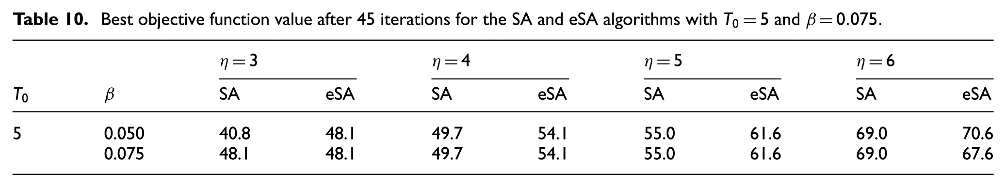
Based on the results in Table 10 and previous testing, we recommend the use of eSA with a higher $T_{0}$ -value and a lower $β$ -value. However, even these results exhibit nuance. For lower values of $η$ (i.e. 3 or 4), $β = 0.075$ was able to improve the GCH objective-value reliably. Similarly, higher $η$ -values of 5 or 6 performed well when $β = 0.05$ .

3.4.2. Additional assets for each asset type

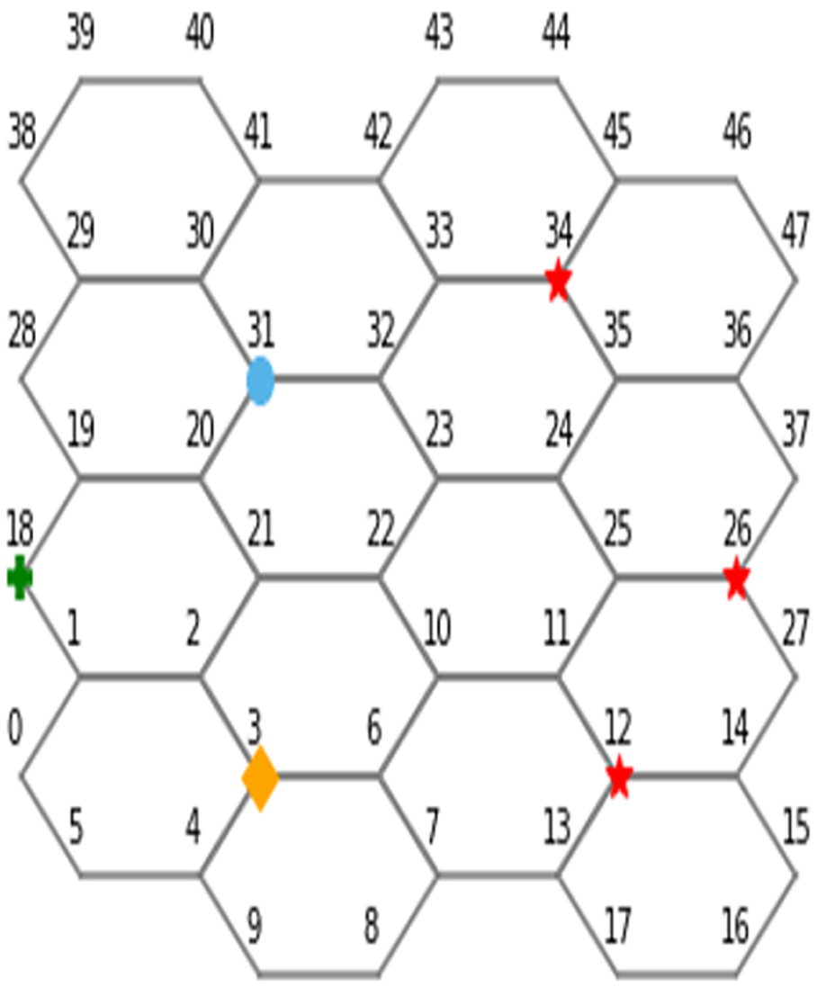
Additional testing explored a modified instance having $K = {1, 2, 3, 4}$ assets and $Ψ = {1, 2}$ asset types, wherein $K_{1} = {1, 2}$ and $K_{2} = {3, 4}$ . Figure 5 depicts the respective origins indicated by the blue circles at Nodes 31 and 41 and orange diamonds at Nodes 3 and 9. All other aspects of the instance are unchanged from Section 3.1. We also restrict our attention to only eSA vis-á-vis GCH, based upon the relatively poorer performance of SA.

Figure 5.

Modified illustrative example: Hexagonal mesh, initial asset locations, and demand node locations.

Figure 6(a) and (b), respectively, presents the asset-routing solutions for no disruptive actions ( $η = 0$ ) and the GCH-identified solution when $η = 5$ . The asset routing is visually different. In Figure 6, assets of type $ψ = 1$ travel directly to demand nodes, whereas assets of type $ψ = 2$ initially meander to allow for sequential servicing of the demands. Moreover, the assets primarily traverse arcs in the middle of the network. In contrast, within Figure 5, where $η = 5$ , most of the disruptive actions slow the travel of assets of type $ψ = 2$ , which no longer meander, although more assets traverse arcs on the boundary of the graph to avoid slower travel.

Figure 6.

Example model execution: additional assets. (a) Routing solution, no delays. (b) Optimal routing $η = 5$ .

For each $η$ -value examined, subsequent pairs of columns within Table 11 report for GCH and eSA (after 45 iterations with $(T_{0}, β) = (5, 0.05)$ ) the best objective function value identified ( $\bar{z}$ ) and the required algorithmic runtime (s).

Table 11.

Best objective function values identified via GCH and eSA after 45 iterations with $(T_{0}, β) = (5, 0.05)$ for the instance depicted in Figure 5 with $| K_{1} | = | K_{2} | = 2$ , for increasing $η$ -values.

	GCH		eSA
$η$	$\bar{z}$	Time (s)	$\bar{z}$	Time (s)
3	34.2	7208.3	35.9	81,075.0
4	34.2	9010.6	41.4	81,081.0
5	36.5	10,812.5	44.9	81,076.0
6	44.2	12,615.0	50.7	81,061.9

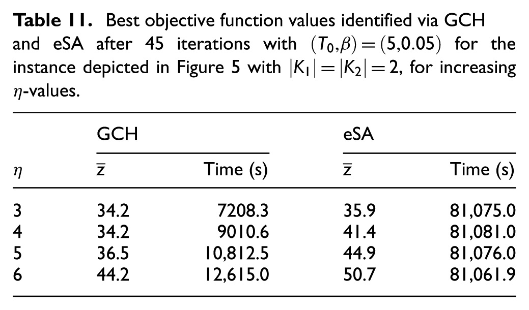
GCH managed smaller improvements as $η$ increased, with no increase between $η = 3$ and $4$ , indicating alternative optimal routing solutions at $η = 3$ . The best objective function found after 45 iterations of eSA consistently improved upon GCH results. The relative (%) improvement in eSA solution quality over GCH solution quality compared with the relative (%) increase in runtime merits discussion. Compared with GCH, eSA attained a minimum, average, and maximum increase in the objective function value by 5.0%, 15.9%, and 23.0%.

This improvement required a 6- to 11-fold increase in runtime. For challenging problem instances, this ratio is foreseeable. The additional asset added to each asset type complicated the solver’s ability to reach optimality for Problem P1 instances, even with a 30-min runtime. Given the time limits, the maximum time to apply GCH for $η$ disruptive actions is $(1 + η) 1800$ s, plus the relatively small amount of time to construct formulations, retrieve solutions, and manage stored information. This equates to $~ 7200$ , $~ 9000$ , $~ 10, 800$ , and $~ 12, 600$ s. Evident from the results in Table 11, Gurobi is terminating due to time limitations for each GCH instance of Problem P1.

Note that the eSA runtime is the runtime after it is initialized with the GCH-identified solution. Given 45 iterations with a 1800 time limit to solve each lower-level problem, the maximum eSA time is $~ 81, 000$ s, plus the time to search the upper-level feasible region, construct formulations, retrieve solutions, and manage stored information. Thus, for eSA instances, Gurobi is again terminating due to time limits. More specifically, each eSA implementation required 22.5 h of runtime, whereas GCH required 2, 2.5, 3, and 3.5 h of runtime for $η = 3, 4, 5, 6$ .

Whereas results presented in Section 3.3 exhibited an average relative optimality gap less than 0.01% for lower-level problem instances, these results averaged 73.9%. Of note, such results do not indicate that the solutions to the lower-level problems are necessarily suboptimal; they demonstrate the solutions to be no worse than indicated, but they may be better. In general, they illustrate the $NP$ -hard nature of the lower-level problem, and Gurobi must be considered as a heuristic under the runtime limitations. This outcome means the follower’s response is heuristically determined, and eSA is best used as an offline planning tool to improve upon a baseline (e.g. GCH-identified) solution, with sufficient time to identify a follower’s best response to accurately evaluate solution quality.

In general, eSA has merit if the planning time to identify disruptive actions allows enough time to use it. However, it is worth noting that eSA found the best improved objective within the first 15 iterations ( $~ 7.5$ h) for $η = 3$ and 6 and within the first 30 iterations ( $~ 15$ h) for $η = 4$ and 5. Moreover, eSA still attained improvements of 17.8% and 19.5% for $η = 4$ and 5 after 15 iterations, so a decision to embrace eSA is not binary. We recommend its use to improve upon GCH solutions for any time that can be afforded to identify a high-quality network disruption strategy.

3.4.3. Additional asset type

$| Ψ | = 3$ An additional experiment examined a test instance to route one of each of $| Ψ | = 3$ different types of assets. Figure 7 presents the instance, for which the only difference from Figure 1 is an additional asset $K_{3} = {3}$ starting at Node 18, depicted via a green cross. This asset has a minimum travel time $τ_{ij 3} = 0.9, \forall (i, j) \in A$ , a fastest speed equal to the average of $τ_{ij 1}$ and $τ_{ij 2}$ .

Figure 7.

Illustrative example: three asset types.

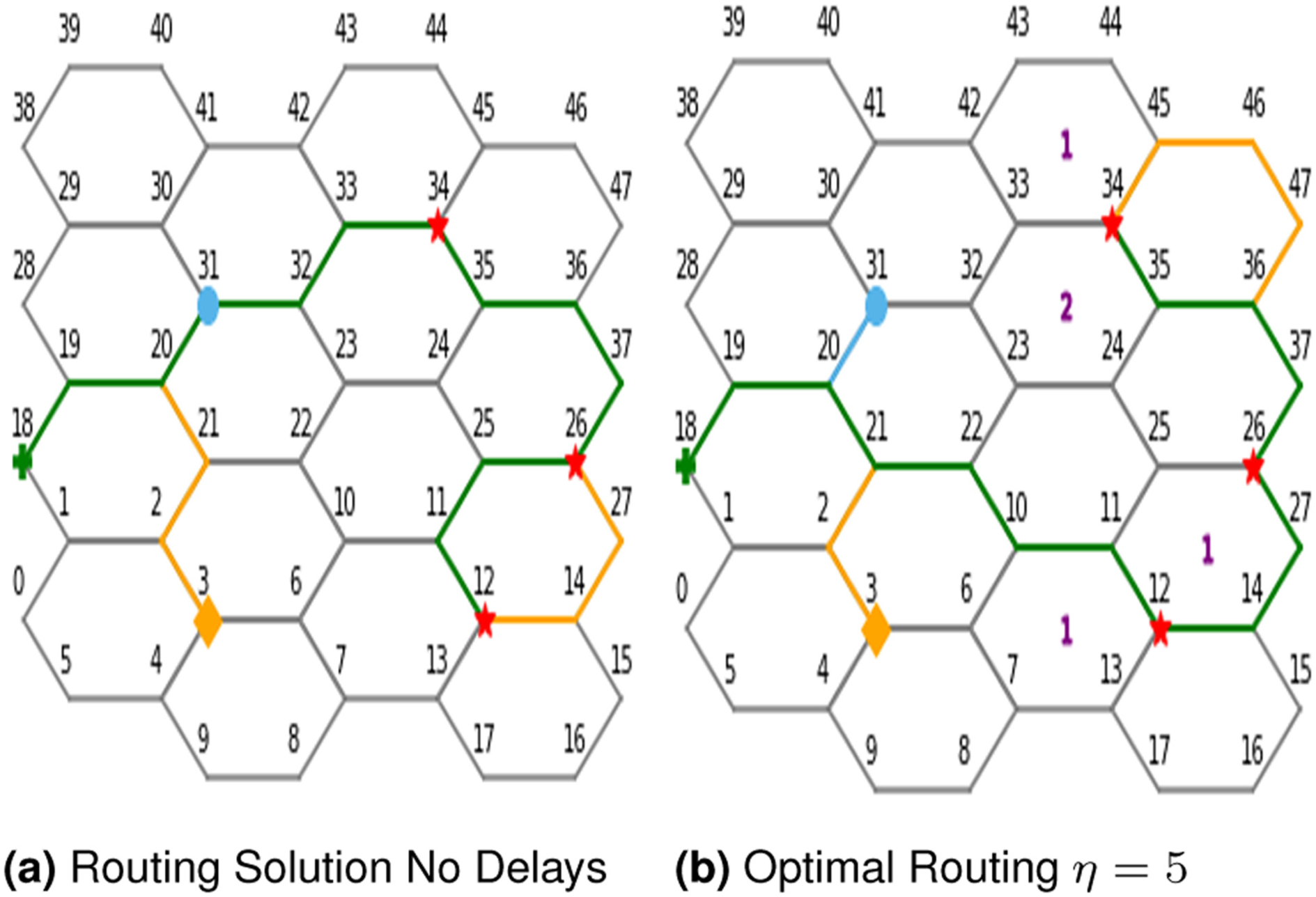
Figure 8(a) and (b), respectively, presents the routing solutions for no disruptive actions ( $η = 0$ ) and the GCH-identified solution when $η = 5$ . Of interest is that both solutions present a routing solution wherein, after each asset reaches a common node (Node 31 in Figure 8(a) and Node 21 in Figure 8(b)), they traverse the same path to the targets, sequenced in ascending order by asset type. A noteworthy difference between the routing solutions is evident with no disruptive actions ( $η = 0$ ) in Figure 8(a); the solution routes assets to service demands at Nodes 34, 26, and 12, in sequence. By comparison, the routing solution in Figure 8(b) (with $η = 5$ ) routes assets to service the demands in reverse order. In the latter solution, the disruptive actions also cause the assets to route on more arcs, including some affected by disruptive actions.

Figure 8.

Example model execution $| Ψ | = 3$ .

Table 12 reports the respective objective function values and runtimes for GCH and eSA, again after 45 iterations with $(T_{0}, β) = (5, 0.05)$ ). Improvement remains consistent over $η = 3, 4, 5$ , with the largest increase in the objective function value occurring when incrementing $η$ from 5 to 6. Thus, the marginal effect of an additional disruptive action does not follow a predictable trend.

Table 12.

Best objective function values identified via GCH and eSA after 45 iterations with $(T_{0}, β) = (5, 0.05)$ for the instance depicted in Figure 7 with $| Ψ | = 3$ asset types, for increasing $η$ -values.

	GCH		eSA
$η$	$\bar{z}$	Time (s)	$\bar{z}$	Time (s)
3	43.2	4414.1	52.2	64,861.6
4	47.4	7245.3	56.7	61,577.5
5	53.8	7768.9	62.7	55,811.9
6	64.2	9569.7	71.7	55,087.5

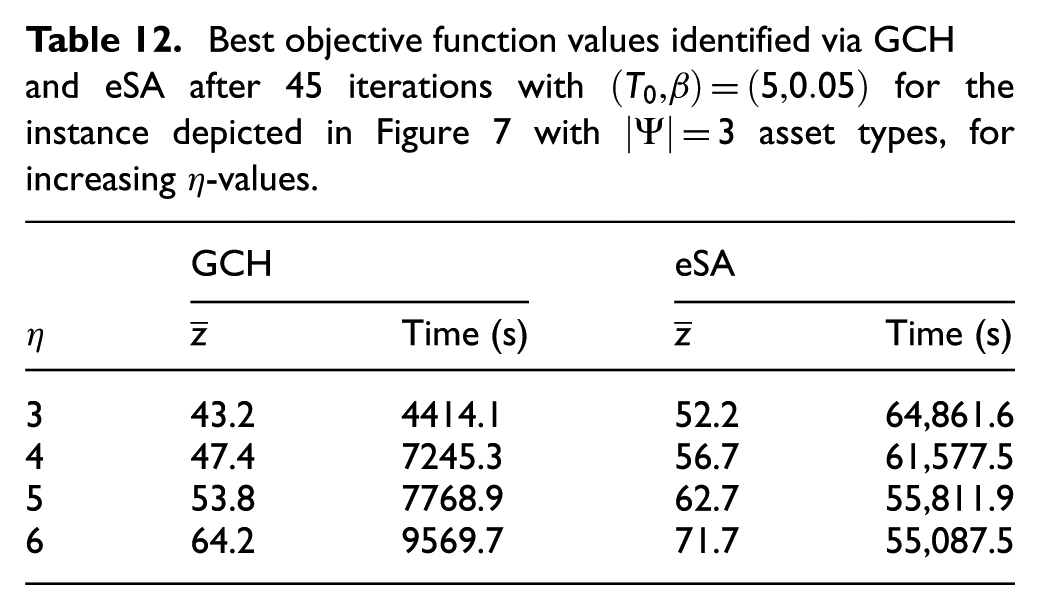
The trade-off between eSA and GCH vis-á-vis solution quality and algorithmic runtime merits discussion. With respect to solution quality, eSA improved upon GCH solutions by a minimum, average, and maximum of 11.7%, 17.3%, and 20.8%, respectively. However, the marginal improvement over GCH strictly declined with an increase in $η$ , indicating the challenge of finding improved solutions for instances with greater complexity.

Interestingly, this marginal decrease with increasing $η$ -values was accompanied by an opposite trend in runtimes. Comparing the runtimes in Table 12 with Table 11, it is evident that Gurobi is not always terminating due to the 1800-s time limit on Problem P1. Although eSA required from 6 to 15 times as much time as GCH to run for 45 iterations, the lower relative increases compared with GCH occurred for larger $η$ -values. Overall, the solutions to the lower-level problems for eSA applied to all $η$ -values were assuredly closer to optimal than those found in Section 3.4.2. The relative optimality gap averaged 7.3% when finding best response routing solutions to identified disruption strategies.

In general, eSA did find improvement within the first 15 iterations; for only one third of the algorithmic runtimes reported in Table 12, eSA improved over GCH by 10.4%, 14.6%, 16.5%, and 3.3%, respectively, for $η = 3, 4, 5,$ and 6. Thus, eSA retains merit for use, even when the larger runtimes are not available to explore the upper-level feasible region more extensively.

4. Conclusions and recommendations

For a subclass of vehicle routing in which multiple asset types are required to service demands in a predetermined sequential order over a contested network, this research formulated the problem as a bilevel program, wherein the lower-level problem routes different types of assets to satisfy demands while minimizing the cumulative service times. Simultaneously, the upper-level problem seeks to identify a strategy that imposes a bounded number of disruptive actions that slow down agent travel on subsets of the network, seeking to maximize the cumulative service time of demands.

This research set forth and evaluated three solution methods: a GCH, a SA metaheuristic, and an enhanced SA that leverages a priority-based candidate solution identification and a tabu list of previously considered solutions. Both simulated annealing-based methods improved upon GCH solutions over a range of problem and algorithmic parameters, with the latter technique doing so more consistently.

Additional testing showed that a larger number of assets of each type was computationally cumbersome, whereas an increased number of asset types was less so. In both excursions, eSA improved the initial solution GCH notably, and it did so within the first 15 iterations (7.5 h) of runtime.

A natural extension of this work would focus on improving the computational effort required to solve the lower-level problem for a fixed disruption strategy. Although outside the scope of this research, decomposition methods merit study. Within Problem P1, the routing of agents is almost separable, except for the sequencing of assets to service each demand within a bounded time window. Such a structure lends itself to subproblems and a restricted master problem, giving promise to improved tractability for these and larger instances, in turn reinforcing the general solution procedure for the bilevel program.

Footnotes

ORCID iD

Stephen D. Donnel

Funding

The authors disclosed receipt of the following financial support for the research, authorship, and/or publication of this article: This research was partially sponsored by the US Transportation Command (USTRANSCOM).

Declaration of conflicting interests

The authors declared no potential conflicts of interest with respect to the research, authorship, and/or publication of this article.

Disclaimer

The views expressed in this article are those of the authors and do not reflect the official policy or position of the US Air Force, the Department of Defense, or the US Government.

Author biographies

Stephen D. Donnel, PhD, is an operations analyst serving in the US Air Force and currently working in the Defense Threat Reduction Agency. He earned his doctorate and Master of Science in operations research from the Air Force Institute of Technology, respectively, in 2023 and 2021.

Brian J. Lunday, PhD, is a professor of Operations Research with the Department of Operational Sciences, Air Force Institute of Technology. He earned his doctorate in industrial and systems engineering from Virginia Tech in 2010 and his Master of Science degree in industrial engineering from the University of Arizona in 2001.

Nicholas T. Boardman, PhD, is an operations analyst serving in the US Air Force and a former Assistant Professor of Operations Research, Air Force Institute of Technology, currently working in the Directorate for Studies and Analysis. He earned his doctorate in industrial engineering from the University of Arkansas in 2021 and his Master of Science degree in operations research from the Air Force Institute of Technology in 2016.

References

Alcazar

Crisis management and the anti-access/area denial problem. Strateg Stud Q 2012; 6(4): 42–70.

Neagoe

Borşa

SS.

Anti-access/area denial strategy–conventional war, hybrid war or asymmetric war?

Strateg Impact. 2019;70/71:15–20. https://www.ceeol.com/search/article-detail?id=853247

Stackelberg

Theory of the market economy. Oxford University Press, 1952.

Dempe

Foundations of bilevel programming. Springer, 2002.

Bard

JF.

Practical bilevel optimization: algorithms and applications. Vol. 30. Springer, 2013.

Moore

Bard

JF.

The mixed integer linear bilevel programming problem. Oper Res 1990; 38(5): 911–921.

Colson

Marcotte

Savard

An overview of bilevel optimization. Ann Oper Res 2007; 153: 235–256.

Smith

Song

A survey of network interdiction models and algorithms. Eur J Oper Res 2020; 283(3): 797–811.

Wood

RK.

Deterministic network interdiction. Math Comput Model 1993; 17(2): 1–18.

10.

Dempe

Kalashnikov

Rıäos-Mercado

RZ.

Discrete bilevel programming: application to a natural gas cash-out problem. Eur J Oper Res 2005; 166(2): 469–488.

11.

Huang

Song

, et al. Optimal sizing and operations of shared energy storage systems in distribution networks: a bi-level programming approach. Appl Energy 2022; 307: 118170.

12.

Albornoz

Vera

PI.

Coordinating harvest planning and scheduling in an agricultural supply chain through a stochastic bilevel programming. Int Trans Oper Res 2023; 30(4): 1819–1842.

13.

Zhang

Zhao

Location planning of electric vehicle charging station with users’ preferences and waiting time: multi-objective bi-level programming model and HNSGA-II algorithm. Int J Prod Res 2022; 61: 1394–1423.

14.

Nunes

Moura

Santos

Solving the multi-objective bike routing problem by meta-heuristic algorithms. Int Trans Oper Res 2023; 30(2): 717–741.

15.

Israeli

Wood

RK.

Shortest-path network interdiction. Networks 2002; 40(2): 97–111.

16.

Lunday

Sherali

HD.

Network interdiction to minimize the maximum probability of evasion with synergy between applied resources. Ann Oper Res 2012; 196: 411–442.

17.

Starita

Scaparra

MP.

Assessing road network vulnerability: a user equilibrium interdiction model. J Oper Res Soc 2021; 72(7): 1648–1663.

18.

Sadati

MEH

Aksen

Aras

The r-interdiction selective multi-depot vehicle routing problem. Int Trans Oper Res 2020; 27(2): 835–866.

19.

Sadati

MEH

Aksen

Aras

A trilevel r-interdiction selective multi-depot vehicle routing problem with depot protection. Comput Oper Res 2020; 123: 104996.

20.

Lei

Shen

Song

Stochastic maximum flow interdiction problems under heterogeneous risk preferences. Comput Oper Res 2018; 90: 97–109.

21.

Perea

Puerto

Revisiting a game theoretic framework for the robust railway network design against intentional attacks. Eur J Oper Res 2013; 226(2): 286–292.

22.

Zokaee

Bozorgi-Amiri

Sadjadi

SJ.

A robust optimization model for humanitarian relief chain design under uncertainty. Appl Math Model 2016; 40(17–18): 7996–8016.

23.

Brown

Carlyle

Salmerón

, et al. Defending critical infrastructure. Interfaces 2006; 36(6): 530–544.

24.

Verter

Dasci

The plant location and flexible technology acquisition problem. Eur J Oper Res 2002; 136(2): 366–382.

25.

Jouzdani

Sadjadi

Fathian

. Dynamic dairy facility location and supply chain planning under traffic congestion and demand uncertainty: a case study of Tehran. Appl Math Model 2013; 37(18-19): 8467–8483.

26.

Laan

Barros

Boucherie

, et al. Optimal deployment for anti-submarine operations with time-dependent strategies. J Def Model Simul 2020; 17(4): 419–434.

27.

Jeroslow

RG.

The polynomial hierarchy and a simple model for competitive analysis. Math Program 1985; 32(2): 146–164.

28.

Musman

Turner

A game theoretic approach to cyber security risk management. J Def Model Simul 2018; 15(2): 127–146.

29.

Hill

Champagne

Price

JC.

Using agent-based simulation and game theory to examine the WWII Bay of Biscay U-boat campaign. J Def Model Simul 2004; 1(2): 99–109.

30.

Harris

Dixon

Dunn

, et al. Simulation modeling for maritime port security. J Def Model Simul 2013; 10(2): 193–201.

31.

Vonk

Kononova

Bäck

, et al. Multi-agent influence diagrams to hybrid threat modeling. J Def Model Simul. Epub ahead of print 20 March, 2025. https://doi.org/10.1177/15485129251315178

32.

Asher

Basak

Fernandez

, et al. Strategic maneuver and disruption with reinforcement learning approaches for multi-agent coordination. J Def Model Simul 2023; 20(4): 509–526.

33.

Niu

Jagannathan

Optimal defense and control of dynamic systems modeled as cyber-physical systems. J Def Model Simul 2015; 12(4): 423–438.

34.

Bard

Moore

JT.

An algorithm for the discrete bilevel programming problem. Nav Res Logist 1992; 39(3): 419–435.

35.

DeNegre

Ralphs

TK.

A branch-and-cut algorithm for integer bilevel linear programs. In: Chinneck

Kristjansson

Saltzman

(eds) Operations research and cyber-infrastructure. Springer, pp.65–78.

36.

Bialas

Karwan

MH.

Two-level linear programming. Manage Sci 1984; 30(8): 1004–1020.

37.

Robbins

Lunday

BJ.

A bilevel formulation of the pediatric vaccine pricing problem. Eur J Oper Res 2016; 248(2): 634–645.

38.

Conn

Gould

Toint

PL.

Trust region methods. Society for Industrial and Applied Mathematics (SIAM), 2000.

39.

Ishizuka

Aiyoshi

Double penalty method for bilevel optimization problems. Ann Oper Res 1992; 34(1): 73–88.

40.

Sahin

Ciric

AR.

A dual temperature simulated annealing approach for solving bilevel programming problems. Comput Chem Eng 1998; 23(1): 11–25.

41.

Yin

Genetic-algorithms-based approach for bilevel programming models. J Transp Eng 2000; 126(2): 115–120.

42.

Calvete

Gale

Mateo

PM.

A new approach for solving linear bilevel problems using genetic algorithms. Eur J Oper Res 2008; 188(1): 14–28.

43.

Wang

Wan

, et al. A globally convergent algorithm for a class of bilevel nonlinear programming problem. Appl Math Comput 2007; 188(1): 166–172.

44.

Kuo

Lee

Zulvia

, et al. Solving bi-level linear programming problem through hybrid of immune genetic algorithm and particle swarm optimization algorithm. Appl Math Comput 2015; 266: 1013–1026.

45.

Shoham

Leyton-Brown

Multiagent systems: algorithmic, game-theoretic, and logical foundations. Cambridge University Press, 2008.

46.

Desrochers

Laporte

Improvements and extensions to the Miller-Tucker-Zemlin subtour elimination constraints. Oper Res Lett 1991; 10(1): 27–36.

47.

Miller

Tucker

Zemlin

RA.

Integer programming formulation of traveling salesman problems. J Assoc Comput Mach 1960; 7(4): 326–329.

48.

Toth

Vigo

The vehicle routing problem. Society for Industrial and Applied Mathematics (SIAM), 2002.

49.

Arora

Barak

Computational complexity: a modern approach. Cambridge University Press, 2009.

50.

Lunday

Sherali

HD.

Minimizing the maximum network flow: models and algorithms with resource synergy considerations. J Oper Res Soc 2012; 63: 1693–1707.

51.

Lessin

Lunday

Hill

RR.

A bilevel exposure-oriented sensor location problem for border security. Comput Oper Res 2018; 98: 56–68.

52.

Nemhauser

DBG

Wolsey

Integer programming and combinatorial optimization. Springer, 1993.

53.

Bard

Falk

JE.

An explicit solution to the multi-level programming problem. Comput Oper Res 1982; 9(1): 77–100.

54.

Kirkpatrick

, Gelatt CD Jr and Vecchi MP. Optimization by simulated annealing. Science 1983; 220(4598): 671–680.

55.

Holland

JH.

Genetic algorithms and the optimal allocation of trials. SIAM J Comput 1973; 2(2): 88–105.

56.

Kennedy

Eberhart

Particle swarm optimization. In: Proceedings of ICNN’95-international conference on neural networks, Vol. 4, Perth, WA, 27 November–1 December 1995. IEEE, pp.1942–1948.

57.

Dorigo

Di Caro

Ant colony optimization: a new meta-heuristic. In: Proceedings of the 1999 congress on evolutionary computation, Vol. 2, Washington, DC, 6–9 July. IEEE, pp.1470–1477.

58.

Glover

Future paths for integer programming and links to artificial intelligence. Comput Oper Res 1986; 13(5): 533–549.

59.

Marques-Silva

Sakallah

KA.

Grasp: a search algorithm for propositional satisfiability. IEEE Trans Comput 1999; 48(5): 506–521.

60.

Osman

IH.

Metastrategy simulated annealing and tabu search algorithms for the vehicle routing problem. Ann Oper Res 1993; 41: 421–451.

61.

Van Breedam

Improvement heuristics for the vehicle routing problem based on simulated annealing. Eur J Oper Res 1995; 86(3): 480–490.

62.

Chiang

Russell

RA.

Simulated annealing metaheuristics for the vehicle routing problem with time windows. Ann Oper Res 1996; 63: 3–27.

63.

Vincent

Redi

Hidayat

, et al. A simulated annealing heuristic for the hybrid vehicle routing problem. Appl Soft Comput 2017; 53: 119–132.

64.

Prihodko

Dai

Zheng

, et al. Multi-objective simulated annealing-based routing plane computation for multiple demands. In: 2022 international conference on modern network technologies (MoNeTec), Moscow, Russian Federation, 27–29 October. IEEE, pp.1–8.

65.

Laporte

Gendreau

Potvin

, et al. Classical and modern heuristics for the vehicle routing problem. Int Trans Oper Res 2000; 7(4–5): 285–300.

66.

Mohammadi

Mahmoodian

Mohammadi

A simulated annealing approach (SA) to vehicle routing problem with time windows (VRPTW). In: 2022 8th international conference on control, instrumentation and automation (ICCIA), Tehran, Iran, 2–3 March. IEEE, pp.1–6.

67.

Janjarassuk

Nakrachata-Amon

A simulated annealing algorithm to the stochastic network interdiction problem. In: 2015 IEEE international conference on industrial engineering and engineering management, Singapore, 6–9 December. IEEE, pp.230–233.

68.

Parsafard

Sensor location design for interdicting mobile travelers with probabilistic space-time trajectories. Transp Res Part C Emerg Technol 2021; 132: 103420.

69.

Osorio-Mora

Rey

Toth

, et al. Effective metaheuristics for the latency location routing problem. Int Trans Oper Res 2023.

70.

Michalopoulos

Barnes

Morton

DP.

Prioritized interdiction of nuclear smuggling via tabu search. Optim Lett 2015; 9: 1477–1494.

71.

Aksen

Aras

A matheuristic for leader-follower games involving facility location-protection-interdiction decisions. In: Talbi

(ed.) Metaheuristics for bi-level optimization. Springer, 2013, pp.115–151.

72.

Yousefi

Donohue

Temporal and spatial distribution of airspace complexity for air traffic controller workload-based sectorization. In: AIAA 4th Aviation Technology, Integration and Operations (ATIO) Forum, Chicago, IL, 20–22 September. AIAA, p.6455.

73.

Lunday

Sherali

Lunday

KE.

The coastal seaspace patrol sector design and allocation problem. Comput Manag Sci 2012; 9(4): 483–514.

74.

Ostrowski

Linderoth

Rossi

, et al. Orbital branching. Math Program 2011; 126: 147–178.

A Stackelberg framework for disrupting coordinated,multi-asset routing and sequential servicing of demands

Abstract

Keywords

1. Introduction

1.1. Problem statement

1.2. Literature review

1.2.1. Bilevel programming

1.2.2. Network interdiction models

1.2.3. Solution methods

1.3. Statement of contributions

2. Model formulation and solution methodology

2.1. Model formulation

2.1.1. Sets

2.1.2. Parameters

2.1.3. Decision variables

2.2. Solution methodology

2.2.1. Greedy construction heuristic

2.2.2. Simulated annealing metaheuristic

2.2.3. Enhanced simulated annealing metaheuristic

3. Testing, results, and analysis

3.1. Illustrative example

3.2. Parameter exploration

3.3. Comparative testing of solution methods

3.4. Selected excursional analyses

3.4.1. Sensitivity analysis for β -values

3.4.2. Additional assets for each asset type

3.4.3. Additional asset type

4. Conclusions and recommendations

Footnotes

ORCID iD

Funding

Declaration of conflicting interests

Disclaimer

Author biographies

References

3.4.1. Sensitivity analysis for $β$ -values