The link between human population dynamics and energy consumption during the Anthropocene

Abstract

Our present world is the consequence of the size of the human population and its domination of the biosphere through the combustion of fossil fuels. Since ~1950, there has been a sudden increase in the rate of human global energy consumption, economic productivity, and population growth. This abrupt departure of the system dynamics has been defined as the “Great Acceleration.” The accelerated population and economic expansion during the past 70 years would have been impossible without using fossil fuels. However, no studies have made an explicit connection between human population dynamics on a global scale and historical changes in energy consumption growth rates, economic growth, and the energy return on investment of fossil fuels (EROI). In this study, I apply a simple population dynamic model of cooperation/competition to decipher the effects of changes in these factors on the dynamics of the human population during the period (1800–2020).

Keywords

energy great acceleration population expansion positive feedback unsustainability

Introduction

The size of the human population and its domination of the biosphere represent the two faces of the enormous problem that the world is facing today (Crutzen, 2002; Crutzen and Stoermer, 2000). Modern civilization has been made possible by the massive and increasing combustion of fossil fuels; the global use of hydrocarbons for human fuel has increased nearly 800-fold since 1750 and approximately 12-fold in the 20th century (Wrigley, 2013). The magnitude of the increase in the rate of human global energy consumption, economic productivity, and population growth has accelerated since ~1950 (Steffen et al., 2007, 2015). Since then, there have been several related changes in the Earth’s system trajectory, such as CO₂ emission rates, upstream sequestration of sediment, the number of synthetic mineral-like compounds, concrete and plastic production, rates of population decline of wildlife species, declines in river runoff, global warming, and accelerated sea-level rise (Syvitski et al., 2020).

This abrupt departure from the temporal pattern of variability in human and Earth System trajectories after ~1950 has been defined as the “Great Acceleration” (Head et al., 2022; Steffen et al., 2007, 2015; Syvitski et al., 2020). The accelerated expansion of the global human population and economies during the past 70 years has only been possible because of the expansion in the use of fossil fuels (Hall, 2017). In fact, the Green Revolution, sustained by the Haber-Bosch process and the improvements in human health based on vaccination programs and medical innovations, are all based on the use of fossil fuels. Combining rapid population growth driven by industrial and technological innovations and energy consumption growth, these two processes make the “Great Acceleration” possible (Fischer-Kowalski et al., 2014). However, we will face two significant problems with the use of fossil fuels. First, oil reserves have been declining since 1970 (Hall, 2017; Hall and Day, 2009; second, there are negative environmental consequences of burning coals and hydrocarbons, such as global warming (Steffen et al., 2018). Much attention is paid to the adverse environmental impacts of fossil fuels. However, less attention is given to the almost total economic and food dependence on this energy source (Hall et al., 2014). Our modern postindustrial high-energy societies are trapped at the crossroads to switch to non-fossil energy sources, but this change carries significant challenges for our lifestyle (Hall, 2017; Hall et al., 2014).

Like all living organisms, human societies are dissipative structures that must gain more energy than they expend in acquiring it. Moreover, the energy return on investment (EROI) is a measure for determining the net energy available to a society to achieve some work. The EROI is the energy gained from a unit of energy spent in obtaining energy (Cleveland et al., 1984; Hall and Cleveland, 1981; Murphy et al., 2011). Moreover, domestic growth, measured as our high-energy societies’ gross domestic product (GDP), is closely related to the EROI changes in fossil fuels (Hall et al., 2014). Several indices of quality of life, such as the human development index, per capita health expenditure, female literacy, and gender inequality, strongly correlate with the societal values of the EROI (Lambert et al., 2014). However, in recent years, some studies have revealed that the EROI, mainly of fossil fuels, and hence the amount of net energy available for society, are declining (Court and Fizaine, 2017; Hall et al., 2014). In addition, most renewable and non-conventional energy alternatives have substantially lower EROI values than fossil fuels (Hall et al., 2014). Therefore, increasing energy output must be diverted to attain the energy needed to run an economy and avoid increasing population pressure and political instability (Turchin, 2016).

Undoubtedly, the tremendous human population expansion and economic growth over the last few centuries have been closely related to the enormous increase in energy extracted from fossil fuel deposits. In fact, from a demographic perspective, it was more than an industrial revolution; it was a hydrocarbon revolution (Smil, 2017). However, no empirical studies have made an explicit connection between the significant expansion of the human population on a global scale and historical changes in energy consumption, economic growth, and energy return on investment (EROI) (see Court and Fizaine, 2017; Taylor and Tainter, 2016). It suggests that the link between available energy and population dynamics in industrial societies has been disrupted (Fischer-Kowalski et al., 2014). However, from a theoretical point of view, it has been proposed that there is a positive feedback loop among niche construction, ecosystem engineering, energy consumption, and human population size (Ellis, 2015; Ellis et al., 2018; Snyder, 2020). Any increase in available energy will support a larger human population, which further increases the rate of technological innovations for energy extraction, causing an unsustainable population expansion (Lima et al., 2024; Snyder, 2020).

Thus, the motivation of this study was to contribute to fill the gap between empirical and theoretical studies by revealing the positive feedback loop that connects the human population’s expansive process during the last 220 years with historical changes in energy consumption and economic growth (Hagens, 2020; Krall, 2023; Taylor and Tainter, 2016). By applying a proper population dynamic model of cooperation/competition (Lima et al., 2024), I describe the structure and dynamics of this expansive system connecting the changes in global energy consumption, economic growth, and the EROI of fossil fuels with the dynamics of the human population during the period 1800–2020, two centuries characterized by the industrial revolution and with relatively reliable data on energy consumption, economic growth, population and the energy return on investment (EROI) of fossil fuels.

Material and methods

Data

Annual human population estimates for the period 1800–2022 were based on Our World in Data (https://ourworldindata.org/grapher/population-past-future?country=~OWID_WRL). The human population data during the period 1950–2022 are from the UN POP from their World Population Prospects 2022.

The time series of global annual energy production and the annual EROI estimates of fossil fuels correspond to the data published by Court and Fizaine (2017) (data were available by personal request to Victor Court). The time series of the gross world product (GWP) are from Maddison (2007) from 1800 to 1950 and from the GWP per capita of The Maddison Project (2013) multiplied by the United Nations (2015) estimates of global population from 1950 to 2015. To obtain GWP estimates for 2015 and 2020 I used the real GWP growth rate of the World Bank (2022). Because of the high interannual variability of the EROI estimates, the annual time series was smoothed by fitting a cubic spline function (Hastie and Tibshirani, 2017). Spar times used to fit cubic spline functions for the annually resolved time series of the energy consumption growth rates, GWP growth rates and the EROI of fossil fuels were smoothed by setting an intermediate spar parameter of 0.67.

I determined the period of major dynamic transitions exhibited by population, economic and energy consumption growth, and the EROI estimates by applying a statistical procedure borrowed from econometrics to detect structural changes in a linear process. I tested deviations from stability in a classical linear regression model of each time series against time assuming that there is one unknown shift point in each time series in time. Basically, I tested the null hypothesis of no structural changes, the regression coefficient is the same during the entire time interval, against the alternative hypothesis that the regression coefficient shift from one stable regression relationship to a different one. Thus, there are two segments in which the regression coefficients are constant. These change points were estimated by using the least squares method, so pre-shift and post-shifts means values were estimated concurrently with the change point (Bai, 1994). I fitted for each time series the linear regression model, assuming one breakpoint by least squares methods using the strucchange library in the R platform (scripts and data fully available).

Population growth models and statistical analyses

I begin with a simple, nonstructured theoretical model describing the effects of intraspecific competition on the dynamics of a population growing in a finite environment (Royama, 2021) that is a time-discrete version of the original continuous-time model of Verhulst (1838).

x_{t + 1} = x_{t} \cdot r_{m} \cdot e^{[- s \cdot (1 - k) \cdot x_{t}]}

(1)

where x_t+₁ is the population size at time t + 1, r_m is the (mean) potential reproductive rates of the individuals (when they have no competitors and resources are fully available), s is the individual resource requirements, and k is a positive constant 0 < k < 1 that reduces the potential reproductive rates each time an additional individual is added to the population; the lower the k value is, the faster the decrease in reproductive rates is Royama (1992, 2021). The model describing the intrapopulation cooperation effects can be represented as the opposite force of equation (1) using the same ecological base as the discrete time step model of cooperation:

x_{t + 1} = x_{t} \cdot r_{m} \cdot e^{[- z \cdot (1 - k^{'}) \cdot \frac{1}{x_{t}}]}

(2)

where r_m is the mean net reproduction rate and z is a positive constant that represents the effect that some environmental hazards impose on the individuals of the population, for example, when some important resources have defenses, or some environmental factor represents a threat. Therefore, in this case, and in opposition to equation (1), k′ is a positive constant 0 < k′ < 1 that increases the potential reproductive rates toward the maximum reproductive rate r_m each time an additional individual is added to the population. The lower the k′ value is, the faster the reproductive rate increases. In fact, both expressions, s(1−k) in equation 1 and z(1−k′) in equation (2), can be written as simple constants c and w, which are the intensity of competition and the amount of cooperation needed to overcome some environmental hazards, respectively. The higher the c value is, the faster the population growth rate decreases with population density. The magnitude of the parameter c is inversely proportional to the resource availability or the commonly named environmental carrying capacity. Otherwise, the higher the w value is, the higher the population size that is needed to increase population growth rates. Because the net rate of change from generation t to t + 1 is measured as the ratio x_t₊₁/x_t = r_t, equations (1) and (2) can be combined in a single model including the effects of both terms, competition, and cooperation, a simple “Malthusian” (Malthus, 1798) and “Boserupian” (Boserup, 1965) model, as follows:

r_{t} = r_{m} \cdot e^{[- c \cdot x_{t} - w \cdot \frac{1}{x_{t}}]}

(3)

For analytical convenience, I write equation (3) in terms of the logarithmic (per capita) reproductive rate log_e (r_t) = R_t, log_e (r_m) = R_m, and log_e (x_t) = X_t as:

R_{t} = R_{m} - c \cdot e^{(X_{t})} - w \cdot e^{(- X_{t})}

(4)

The shape of the reproductive curve R–X is determined only in terms of these three parameters R_m (the logarithmic (mean) maximum reproductive rate), c (intensity of intrapopulation competition or earth’s carrying capacity) and w (intensity of cooperation), which all have a clear ecological and population dynamic interpretation.

The model of equation (4) can be modified to introduce the effects of exogenous variables, global energy consumption, the growth rate of global energy consumption, the GWP growth rate and the historical EROI estimates on the parameter (c) by assuming a simple linear function effects of each factor on this parameter,

R_{t} = R_{m} - (c + α \cdot z_{t}) \cdot e^{(X_{t})} - w \cdot e^{(- X_{t})}

(5)

where z_t represents the included factor (global energy consumption, global energy consumption growth rates, GWP growth rates and historical EROI of fossil fuels) and the parameter α is the effect on the intensity of intrapopulation competition. The parameter α can be interpreted as how the energy consumption, the gross world product (GWP), the GWP growth rates, the energy consumption growth rates and the EROI of fossil fuels modifies the resource density or the global amount of resources/energy available for the human population. Therefore, negative α values decreased the intensity of intra-population competition, in other words, increase the per capita resource/energy share or individual well-being with changes in the energy, economic and EROI changes.

I fitted the log-transformed time series to equation (5) with nonlinear regressions using the nls (nonlinear least squares) library in the R programing language. Models were ranked according to the second-order Akaike’s information criterion (AICc, see Bumham and Anderson, 2003 for details), and I calculated the Akaike’s weights (w_i) to infer the relative likelihood of each model (Bumham and Anderson, 2003). Finally, using a multimodel inference approach (Symonds and Moussalli, 2011), I estimated the relative importance of each predictor across all candidate models and identified the variable(s) that might be driving the system’s dynamics. This enables quantifying the probability that a given hypothesis is explaining the observed dynamics. It is important to note that in the case of nonlinear models, the R² calculated for each model cannot be used to determine goodness of fit or model performance (Kva°Lseth, 1983), and consequently, I focused primarily on the AIC_c and w_i results.

I compare and validate the models by simulating the total trajectory predictions initiated with the first observed value of the time series and running the algorithm using each model with their estimated parameters to obtain the time series’ remaining simulated values. The accuracy of predictions was assessed using the coefficient of prediction σ² (Turchin et al., 2018),

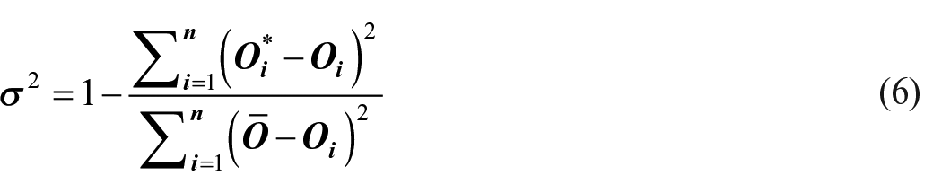
σ^{2} = 1 - \frac{\sum_{i = 1}^{n} {(O_{i}^{*} - O_{i})}^{2}}{\sum_{i = 1}^{n} {(\bar{O} - O_{i})}^{2}}

(6)

O_i indicates observed data from the testing dataset, O_i^* denotes the model predictions, ‾Ο is the mean of the observations, and n is the number of data to be predicted. The coefficient of prediction σ² is 1 when the predicted data are equal to the observed data, 0 when the regression model predicts the data average, and negative if the predictions of the model are worse than the data mean (scripts and data fully available).

Results

In Figure 1a, the series of solid circles is the global human population numbers from 1800 to 2020 plotted in logarithms. The data exhibit an increase with a steadily decreasing rate from 1800 to 1855, there is a significant breaking point (population shift) during the year 1950 (electronic Supplemental Material; Figure S1), and a final acceleration/deacceleration phase from 1950 to 2020. In Figure 1b, the time series of the log_e-reproductive rate (R_t) showed two different phases with a clear temporal breaking point around the year 1945 (electronic Supplemental Material; Figure S1). I transformed the time-plot representation of Figure 1a into the R–X reproduction curve; the resultant plot provides details of human global population changes during the last 220 years that are not visible in the time-plot representation (Figure 1a and b). First, the per-capita rate of change (logarithmic reproduction curve) of the global population over these two centuries showed a humped-like shape following the predictions of the competition/cooperation population dynamic model (Equation 5 and solid line; Figure 1c). Second, the observed log_e-reproductive rate R_t exhibits considerable variation in comparison with the much smoother time-plot representation in Figure 1a. For example, there seem to be two different population waves of acceleration/deacceleration of growth rates during the periods 1800–1945 and 1950–2020 (Figure 1c). In Figure 2, I show the time trajectories of the global annual energy consumption (Figure 2a), the growth rate of the global annual energy consumption (Figure 2b), the gross world product (GWP) (Figure 2c), the growth rate of the GWP (Figure 2d) and the energy return on investment estimates of fossil energy (Figure 2e). The global annual energy consumption showed a significant breaking point during 1950 (electronic Supplemental Material; Figure S1), with a steady and slow increasing trend during the period 1800–1950 and then a sudden acceleration until 2000 (Figure 2a). The growth rates of global annual energy consumption showed an abrupt and significant shift by 1940 (electronic Supplemental Material; Figure S1), the trajectory showed an accelerated increasing trend during the 19th century, a decline from 1900 to 1925, a strong increasing phase during the period 1925–1965, and a last declining trend (Figure 2b). The significant shifting transition of the gross world product (GWP) time series occurred during 1950 (Figure 2c, electronic Supplemental Material; Figure S1), which is consistent with the abrupt and significant shift exhibited by the growth rates of the GWP during 1945 (Figure 2d, electronic Supplemental Material; Figure S1). Finally, the EROI estimates of fossil energy showed a major structural change (significant breaking point) during 1940 (Figure 2e, electronic Supplemental Material; Figure S1). The EROI of fossil energy were relatively low during the first 30 years of the 19th century, they increased rapidly and were relatively stable around a value of 25 during the period 1845–1930, a second increase of EROI values are observed during the period 1935–1970, and a decreasing trend since then (Figure 2e).

Figure 1.

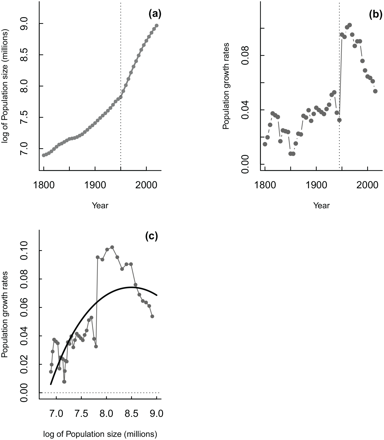
Graphical representation of the global human population size data (solid circles) in a common log-transformation format. (a) Time series of the log-transformed data; vertical dotted lines denote the timing of a major demographic transition in the time series, estimated by using the least squares method, so pre-shift and post-shifts means population size values were estimated concurrently with the change point (electronic Supplemental Material, Figure S1). (b) Time series of the logarithmic net reproductive rates (R_t) of the global human population size; vertical dotted lines denote the timing of a major demographic transition in the time series, estimated by using the least squares method, so pre-shift and post-shifts means population growth rates values were estimated concurrently with the change point (electronic Supplemental Material, Figure S1). (c) Transformation of (a) into a reproduction curve in the R–X format. The solid line is the predicted curve for the “pure” endogenous model from equation (4).

Figure 2.

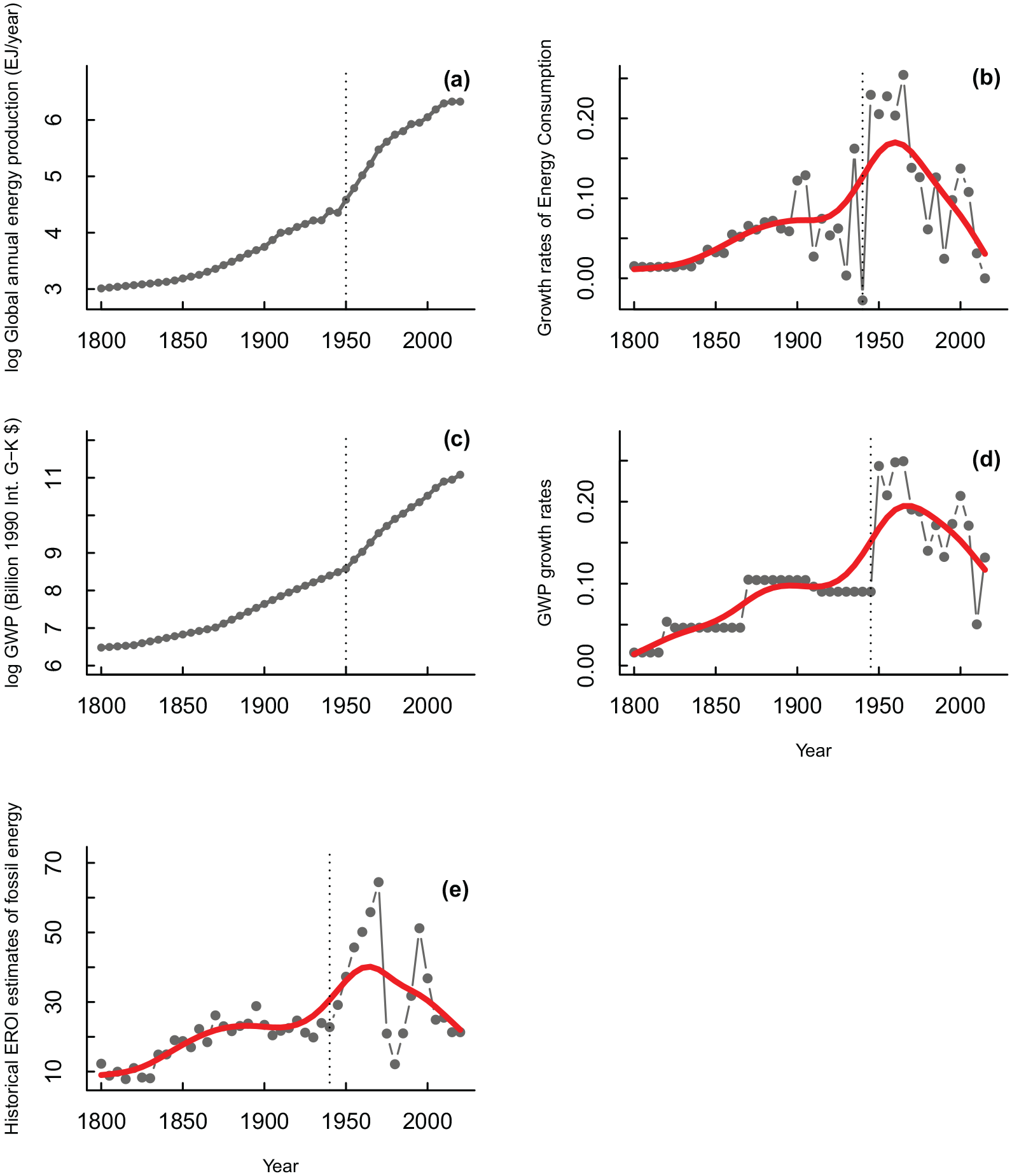
Time series of the energy and economic variables. (a) The time series of global energy consumption in Exajoules/year. (b) The time series of the global energy consumption growth rates. (c) Time series of the gross world product (GWP) in billion international Geary–Khamis 1990 dollars. (d) Time series of the growth rate of GWP. (e) Time series of the historical energy return on investment (EROI) of fossil fuels. Vertical dotted lines denote the timing of a major demographic transition in each time series, estimated by using the least squares method, so pre-shift and post-shifts means values were estimated concurrently with the change point (electronic Supplemental Material, Figure S1). The red lines are the smoothed time series data by applying a cubic spline function (Hastie and Tibshirani, 2017).

In fact, population growth, global annual energy consumption growth rates, GWP growth rates and the EROI values of fossil fuels are all significant and positively correlated (Figure 3a–f and Table 1).

Figure 3.

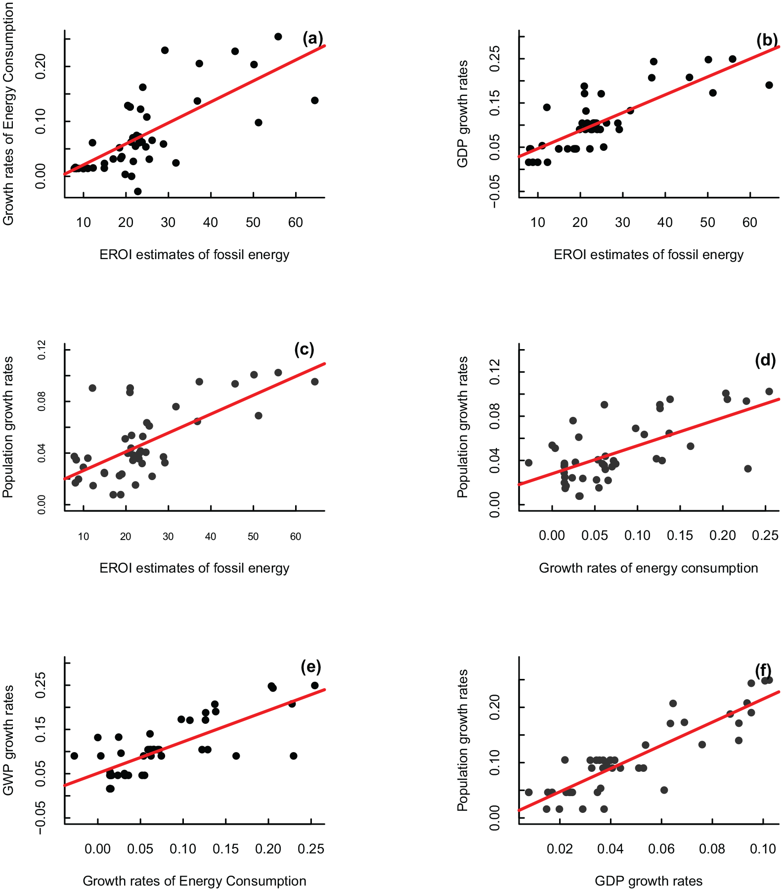
Linear regression plots between: (a) energy return on investment (EROI) of fossil fuels and global energy consumption growth rates (line fitted by linear regression; (y = −0.017 + 0.004x, F_1,42 = 40.8, p < 0.0001, r² = 0.48); (b) energy return on investment (EROI) of fossil fuels and GWP growth rates (y = 0.0062 + 0.0041x, F_1,42 = 73.2, p < 0.0001, r² = 0.63); (c) energy return on investment (EROI) of fossil fuels and population growth rates (y = 0.012 + 0.0015x, F_1,42 = 36.71, p < 0.0001, r² = 0.45); (d) global energy consumption growth rates and population growth rates (y = 0.028 + 0.253x, F_1,42 = 30.3, p < 0.0001, r² = 0.41); (e) global energy consumption growth rates and GWP growth rates (y = 0.051 + 0.710x, F_1,42 = 57.5, p < 0.0001, r² = 0.57); (f) GWP growth rates and population growth rates (y = 0.009 + 0.368x, F_1,42 = 143.5, p < 0.0001, r² = 0.77).

Table 1.

Correlation matrix coefficients (Pearson’s coefficients) between population growth rates, GWP growth rates, energy consumption growth rates and the EROI of fossil energy.

	Population growth rates	GWP growth rates	Energy consumption growth rates	EROI fossil energy
Population growth rates	1	0.88	0.65	0.68
GWP growth rates	0.88	1	0.76	0.80
Energy consumption growth rates	0.65	0.76	1	0.70
EROI fossil energy	0.68	0.80	0.70	1

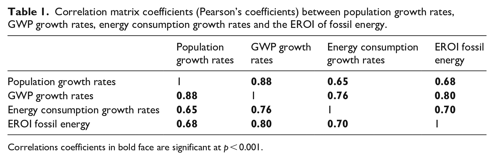
Correlations coefficients in bold face are significant at p < 0.001.

The simple model from equation (4) was not a good predictor of the more complex population growth changes during the industrial revolution (Table 2), suggesting that some other factors must be considered in the model. In fact, the predicted logarithmic growth rates dynamic was not able to capture the sudden observed changes (Figure 4a). The population model including the historical global energy consumption data (Court and Fizaine, 2017) as a forcing term in the parameter c from equation (5) improves the model fit compared with the pure competition/cooperation model (Table 2 and Figure 4b). However, the sign of the effect (positive) indicates that increases in energy consumption shift the Earth’ human carrying capacity toward lower values, which is inconsistent with the theoretically expected results. The model could not predict two essential features of the population growth rate pattern (Table 2). First, relatively constant values were exhibited during almost a century (1850–1945), and second, a sudden increase was observed during the “Great Acceleration” phase (1950–1970). In contrast, the predictions showed a monotonic increase in the R–X plane and a sudden decrease (Figure 4b). In the same vein, the population model including the GWP as a forcing term in the parameter c of equation (5) (economic wealth as a proxy of earth carrying capacity) was no able to capture the two essential features described above (Table 2 and Figure 4c).

Table 2.

Population models (equation (5)) fitted to the population size time series from the global human population data. Model A: includes a pure endogenous dynamic ( $R_{t} = R_{m} - c \cdot e^{(X_{t})} - w \cdot e^{(- X_{t})}$ ). Model B: the effect of global energy consumption (Exajoules) on the parameter c ( $R_{t} = R_{m} - (c + α \cdot E n e r g y_{t}) \cdot e^{(X_{t})} - w \cdot e^{(- X_{t})}$ ). Model C: the effect of the gross world product (GWP) on parameter c ( $R_{t} = R_{m} - (c + α \cdot G W P_{t}) \cdot e^{(X_{t})} - w \cdot e^{(- X_{t})}$ ). Model D: the effect of the growth of energy consumption (smoothed) on parameter c ( $R_{t} = R_{m} - (c + α \cdot E n e r g y g r o w t h_{t}) \cdot e^{(X_{t})} - w \cdot e^{(- X_{t})})$ . Model E: the effect of GWP growth (smoothed) on parameter c ( $R_{t} = R_{m} - (c + α \cdot G W P g r o w t h_{t}) \cdot e^{(X_{t})} - w \cdot e^{(- X_{t})}) .$ Model F: the effect of EROI of fossil fuels (smoothed) on parameter c ( $R_{t} = R_{m} - (c + α \cdot E R O I_{t}) \cdot e^{(X_{t})} - w \cdot e^{(- X_{t})}$ ). Parameter values are given in the columns of the table. The model notations are as follows: R_m is the logarithmic (mean) maximum reproductive rate, c is the intensity of intrapopulation competition, w is the amount of cooperation needed to overcome some environmental hazards, and α₁, α₂, and α₃ are the effects of energy consumption, growth of the energy consumption and the EROI of fossil fuels on c. AIC_c indicates the Akaike information criteria corrected for the small sample size, w_i is Akaike’s weights and σ² is the coefficient of prediction (equation (6)).

Model	R_m	c	w	α₁	AICc	∆ $A I C_{c}$	w_i	σ²
A	0.12	0.00004	104.8		−229.53	31.75	0.00	0.53
B	−0.057	−0.00005	−25.88	6.8 × 10⁻⁰⁸	−243.08	18.20	0.00	0.59
C	0.012	−0.00003	20.49	3.6 × 10⁻¹¹	−241.93	19.35	0.00	0.58
D	0.023	1.8 × 10 ⁻⁶	0.962	−0.00013	−261.28	0.00	0.76	0.79
E	0.066	2.17 × 10⁻⁵	28.70	−0.00016	−257.40	3.88	0.11	0.78
F	0.049	2.35 × 10⁻⁶	15.39	−9.30 × 10⁻⁷	−257.66	3.62	0.12	0.77

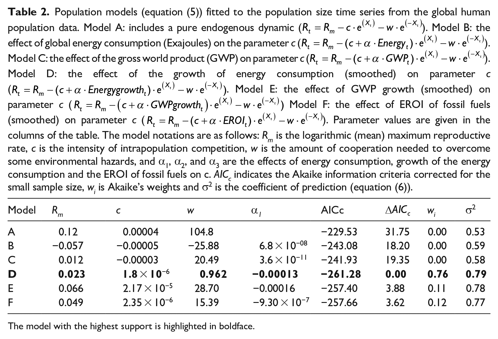
The model with the highest support is highlighted in boldface.

Figure 4.

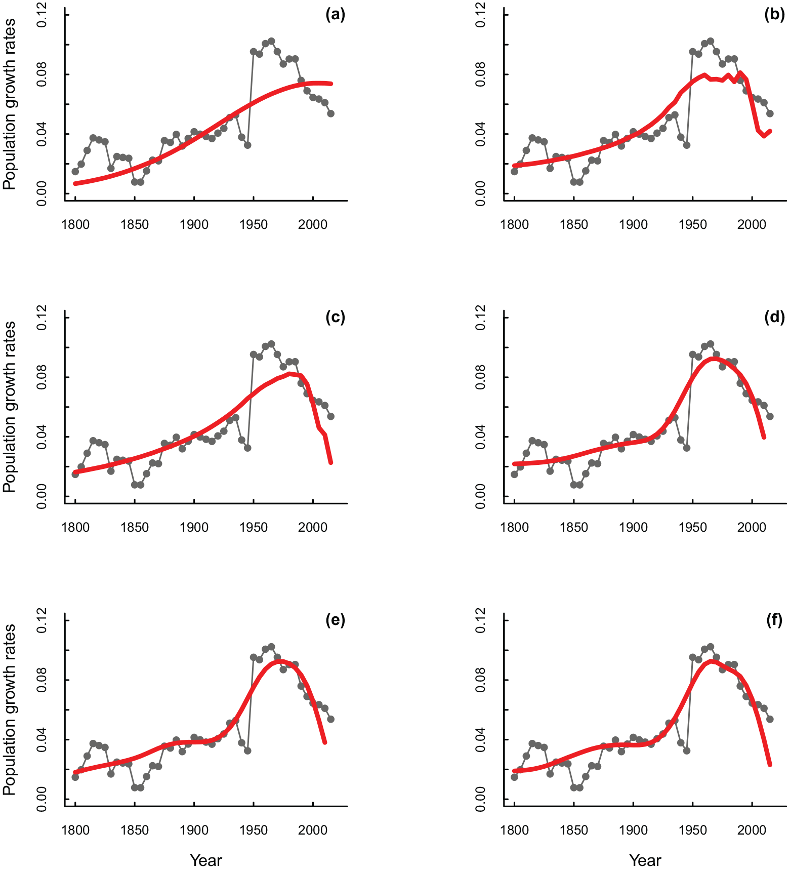
Comparisons between the model predictions (red line) and observed data (gray dots and lines) of the logarithmic population growth rates for: (a) Model A; (b) Model B; (c) Model C; (d) Model D; (e) Model E; and (f) Model F. Models validation and parameters values in Table 2.

The population model, including the growth rates of the global energy consumption as a covariable in the parameter c, was the best model according to the AICc values, the Akaike’s weights and the coefficient of prediction (Table 2). This result is supported by the cumulative w_i, indicating that this model has a very high probability (76%) of being included as the best model, compared with the support for the competing models. In addition, the sign of the effect (negative) suggests that increases in the growth rate of energy consumption decrease the intensity of competition as a “lateral” perturbation effect (sensu (Royama, 1992)) (Table 2). This “lateral” perturbation effect can be interpreted as an increase of the Earth’ carrying capacity caused by high values of the growth rates of energy consumption. In fact, model predictions captured some essential features of the observed logarithmic population growth rate dynamics, for example, the positive and relatively constant population growth rate trend observed during 1845–1945 and the rapid acceleration of population growth rates observed from 1950 to 1970 (Figure 4d). The population models including the growth rates of GWP and the EROI of fossil energy as covariables in the parameter c, were also very good models according to the AICc values, the Akaike’s weights and the coefficient of prediction (Table 2). Both models also captured the same essential features of the observed logarithmic population growth rates R_t, (Figure 4e and f). Because of the high correlation between the growth rates of energy consumption, GWP growth rates, and EROI of fossil energy, increases in these variables represent a “lateral” perturbation effect that can be interpreted as an increase in the Earth’s carrying capacity.

Discussion

Understanding how human population, energy, and economic growth are connected is one of the main questions to be resolved in the 21st century, both in ecology and the social sciences. It has been argued that in industrial societies, the link between energy availability and population dynamics has been disrupted (Fischer-Kowalski et al., 2014). However, the results of this study suggest that the expansion of the global human population during the last two centuries has been primarily interdependent with energy consumption, the changes in the EROI of fossil energy, and the economic growth rates. In sum, population dynamics, energy, and economic growth rates are engaged in a positive feedback loop explaining the expansionary dynamics exhibited by our population and economic system (Krall, 2022, 2023; Taylor and Tainter, 2016).

Using a simple theoretical population dynamic model, the effects of EROI of fossil energy, energy, and economic growth on parameter c from equation (5) can be interpreted as nonadditive effects of free energy for economic growth on human population dynamics. In other words, higher values of energy consumption growth, economic growth, and the EROI of fossil fuels can be interpreted as an increase in the Earth’s carrying capacity for humans, which is the classic “lateral” perturbation effect described by Royama (1992, 2021). The same modeling procedure has helped link the effects of long-term climate change and agricultural production in agrarian societies (Gayo et al., 2024; Lima, 2014; Lima et al., 2020).

However, the problem of expansionary and interdependent systems is when they reach their limits. Because of the nonadditive “lateral” perturbations effects (Royama, 1992) of energy consumption growth rates, EROI of fossil energy, and economic growth, even small decreases in any of these factors can trigger disproportionately large demographic responses when the population size is considerable. This occurs because independent of the magnitude of future changes in energy consumption growth rates, EROI of fossil fuels, or economic growth. The population dynamic theory predicts that their impact is modulated by the population size, mainly through a per-capita energy-economic growth share (Royama, 1992). This result suggests that any increase in population size in the presence of diminishing returns of energy and economic growth makes our present human societies increasingly vulnerable to collapse or simplification (Hagens, 2020; Tainter, 1988; Taylor and Tainter, 2016). The population dynamic model used here is consistent with humans’ propensity toward unsustainability (Snyder, 2020).

Therefore, the results of this study suggest that the previous expansive dynamics of this highly interdependent system, population, energy, and economic growth, could constrain the potential shared socioeconomic pathways (SSPs) (O’Neill et al., 2014). The five different SSPs narratives, such as sustainable development, regional rivalry, inequality, fossil-fueled development, and middle-of-the-road development (Riahi et al., 2017), would be severely constrained or changed if population, energy, and economic growth dynamics function as a positive feedback loop.

The population expansion exhibited by the global human population during the last 220 years was not a single demographic process. In contrast, it seems better represented by a sudden change in population growth. Human population growth rates increased by ~0.8%/year in a noisy and almost linear fashion with a log of population size during almost 145 years, which agrees with the period named the industrial interval (1850–1950, Syvitski et al., 2020). This first wave of human population expansion during the Industrial Revolution can be associated with the increases in the total factor of productivity caused by a series of innovations related to the coal-powered steam engine, which has been described as the first cycle of the Industrial Revolution (1750–1900) (Bonaiuti, 2018).

Although there is a trend to think that technology alone will drive the increase in the production of industrial economies for the foreseeable future (next 100 years), the vision of expansive economies and societies is nothing but fairy tales (Smil, 2017). However, between 1950 and 1970, human population growth rates increased almost three times, triggering an extraordinary outburst of consumption and productivity, and driving a cascade of physical, chemical, and biological changes to the Earth that can be used for a new epoch, the Anthropocene (Crutzen, 2002; Syvitski et al., 2020). This abrupt increase in population growth occurred during the middle of the 20th century and appears to be explained by a corresponding abrupt increase in energy consumption growth rates and the EROI of fossil energy around 1930–1940 (Court and Fizaine, 2017). Energy consumption growth rates and the EROI of fossil fuels showed an abrupt and significant shift around 1940, 5–10 years earlier than the economic and population growth breaking points, suggesting that energy changes seem to predate economic and population growth. In fact, during the next decade, global economic productivity showed the highest growth rates of the 20th century (Bonaiuti, 2018). The impressive jump in population growth rates occurred after 1945, which seems to be strongly related to all other changes that occurred post-1950 across different socioeconomic and biophysical variables, which have been named the “Great Acceleration” (Steffen et al., 2015). However, the general trend of the global energy consumption growth rates and the EROI suggests that the amount of energy available to society has been in a general decline during the last decades (Hall et al., 2014). Some authors have estimated that the minimum EROI needed to run modern industrial-consumer societies should be approximately 15–20: 1 if we can support our present way of life (Lambert et al., 2014).

Conclusion

Over the last two centuries, the global human population has experienced two waves of accelerated growth rates, closely related to changes in energy growth, EROI values of fossil fuels, and economic growth. Interestingly, the accelerated population growth of our present industrial society showed the same structural dynamic signature, a humped reproduction curve describing a cooperation/competition process, exhibited during most of the previous historical transitions but powered by a new rich energy source, that is, fossil fuels (Lima et al., 2024). Thus, the structural instability of cooperation/competition dynamics fueled by a new energy source is the signature of population transitions in human societies and may be the ultimate cause of the human propensity toward unsustainability and socio-ecological collapse (Snyder, 2020).

However, a limitation of this study is the use of a simple population dynamic model, which does not include the underlying complexities and differences in population density, energy consumption patterns, and economic growth across the world’s different societies. I am not proposing a causal connection between population, energy, and economic factors; I have described the interdependent dynamics underlying these factors. The energetic stock of fossil fuels supported our recent expansive population process, and future limitations in energetic supply will make our expansive global society vulnerable to diminishing returns (Tainter, 1988; Taylor and Tainter, 2016). The results of this study showed that we are embedded in a complex population, energetic and economic positive feedback loop operating in a finite ecological world. This positive feedback loop should be explicitly considered in the future projected population and socioeconomic stability scenarios under the unprecedented transformations in the functioning of the Earth System (Efferson et al., 2024; Lenton and Scheffer, 2024).

Supplemental Material

sj-docx-1-anr-10.1177_20530196241255081 – Supplemental material for The link between human population dynamics and energy consumption during the Anthropocene

Supplemental material, sj-docx-1-anr-10.1177_20530196241255081 for The link between human population dynamics and energy consumption during the Anthropocene by Mauricio Lima in The Anthropocene Review

Footnotes

Funding

The author(s) disclosed receipt of the following financial support for the research, authorship, and/or publication of this article: This research was supported by the Center of Applied Ecology and Sustainability (CAPES; ANID PIA/BASAL FB0002) and FONDECYT Project #1230075.

ORCID iD

Mauricio Lima

Data availability

The author will provide full accessibility to the data used in the article.

Code availability

The R-script codes are available upon request to the author.

Supplemental material

Supplemental material for this article is available online.

References

Bai

(1994) Least squares estimation of a shift in linear processes. Journal of Time Series Analysis 15(5): 453–472.

Bonaiuti

(2018) Are we entering the age of involuntary degrowth? Promethean technologies and declining returns of innovation. Journal of Cleaner Production 197: 1800–1809.

Boserup

(1965) The Conditions for Agricultural Growth: The Economics of Agrarian Change Under Population Pressure. London: Aldine.

Bumham

Anderson

(2003) Model Selection and Multimodel Inference: A Practical Information-Theoretic Approach. Berlin: Springer Science and Business Media.

Cleveland

Costanza

Hall

, et al. (1984) Energy and the U.S. economy: A biophysical perspective. Science 225(4665): 890–897.

Court

Fizaine

(2017) Long-term estimates of the energy-return-on-investment (EROI) of coal, oil, and gas global productions. Ecological Economics 138: 145–159.

Crutzen

Stoermer

(2000) The “anthropocene”. Global Change Newsletter 41: 17.

Crutzen

(2002) Geology of mankind. Nature 415: 23.

Efferson

Richerson

Weinberger

(2024) Our fragile future under the cumulative cultural evolution of two technologies. Philosophical Transactions of the Royal Society A: 379: 20220257.

10.

Ellis

(2015) Ecology in an anthropogenic biosphere. Ecological Monographs 85: 287–331.

11.

Ellis

Magliocca

Stevens

, et al. (2018) Evolving the anthropocene: Linking multi-level selection with long-term social-ecological change. Sustainability Science 13: 119–128.

12.

Fischer-Kowalski

Krausmann

Pallua

(2014) A sociometabolic reading of the anthropocene: Modes of subsistence, population size and human impact on Earth. Anthropocene Review 1(1): 8–33.

13.

Gayo

Lima

Gurruchaga

, et al. (2024) Towards understanding human–environment feedback loops: The Atacama Desert case. Philosophical Transactions of the Royal Society A: 379: 20220253.

14.

Hagens

(2020) Economics for the future – Beyond the superorganism. Ecological Economics 169: 106520.

15.

Hall

(2017) Energy Return on Investment. A Unifying Principle for Biology, Economics, and Sustainability. Syracuse, NY: Springer.

16.

Hall

Cleveland

(1981) Petroleum drilling and production in the United States: Yield per effort and net energy analysis. Science 211: 576–579.

17.

Hall

CAS

Lambert

Balogh

(2014) EROI of different fuels and the implications for society. Energy Policy 64: 141–152.

18.

Hall

Day

(2009) Revisiting the limits to growth after peak oil: In the 1970s a rising world population and the finite resources available to support it were hot topics. Interest faded—But it’s time to take another look. American Scientist 97: 230–237.

19.

Hastie

Tibshirani

(2017) Generalized Additive Models. Milton Park: Routledge.

20.

Head

Steffen

Fagerlind

, et al. (2022) The great acceleration is real and provides a quantitative basis for the proposed anthropocene series/epoch. International Union of Geological Sciences 45: 359–376.

21.

Krall

(2022) Bitter Harvest: An Inquiry Into the War Between Economy and Earth. Albany, NY: State University of New York Press.

22.

Krall

(2023) The economic superorganism in the complexity of evolution. Philosophical Transactions of the Royal Society A: 378: 20210417.

23.

Kva°Lseth

(1983) Note on the R2 measure of goodness of fit for nonlinear models. Bulletin of the Psychonomic Society 21(1): 79–80.

24.

Lambert

Hall

CAS

Balogh

, et al. (2014) Energy, EROI and quality of life. Energy Policy 64: 153–167.

25.

Lenton

Scheffer

(2024) Spread of the cycles: A feedback perspective on the anthropocene. Philosophical Transactions of the Royal Society A: 379: 20220254.

26.

Lima

(2014) Climate change and the population collapse during the “great famine” in pre-industrial Europe. Ecology and Evolution 4(3): 284–291.

27.

Lima

Gayo

Estay

, et al. (2024) Positive feedbacks in deep-time transitions of human populations. Philosophical Transactions of the Royal Society A: 379: 20220256.

28.

Lima

Gayo

Latorre

, et al. (2020) Ecology of the collapse of rapa nui society. Proceeding of the Royal Society B 287(1929): 20200662.

29.

Malthus

(1798) An essay on the principle of population as its affects the future improvement of society: with remarks on the speculations of Mr. Godwin, M. Condorcet, and other writers. London: J. Johnson.

30.

Murphy

Hall

CAS

Dale

, et al. (2011) Order from chaos: A preliminary protocol for determining the EROI of fuels. Sustainability 3: 1888–1907.

31.

O’Neill

Kriegler

Riahi

, et al. (2014) A new scenario framework for climate change research: The concept of shared socioeconomic pathways. Climatic Change 122: 387–400.

32.

Riahi

van Vuuren

Kriegler

, et al. (2017) The shared socioeconomic pathways and their energy, land use, and greenhouse gas emissions implications: An overview. Global Environmental Change 42: 153–168.

33.

Royama

(1992) Analytical Population Dynamics. Berlin: Springer Science & Business Media.

34.

Royama

(2021) Animal Population Ecology: An Analytical Approach. Cambridge: Cambridge University Press.

35.

Smil

(2017) Energy: A Beginner’s Guide. New York, NY: Simon and Schuster.

36.

Snyder

(2020) The genetic and cultural evolution of unsustainability. Sustainability Science 15: 1087–1099.

37.

Steffen

Broadgate

Deutsch

, et al. (2015) The trajectory of the anthropocene: The great acceleration. Anthropocene Review 2(1): 81–98.

38.

Steffen

Crutzen

McNeill

(2007) The anthropocene: Are humans now overwhelming the great forces of nature. Ambio-Journal of Human Environment Research and Management 36(8): 614–621.

39.

Steffen

Rockström

Richardson

, et al. (2018) Trajectories of the earth system in the anthropocene. Proceedings of the National Academy of Sciences 115: 8252–8259.

40.

Symonds

MRE

Moussalli

(2011) A brief guide to model selection, multimodel inference and model averaging in behavioural ecology using akaike’s information criterion. Behavioral Ecology and Sociobiology 65: 13–21.

41.

Syvitski

Waters

Day

, et al. (2020) Extraordinary human energy consumption and resultant geological impacts beginning around 1950 CE initiated the proposed anthropocene epoch. Communications Earth and Environment 1: 32.

42.

Tainter

(1988) The Collapse of Complex Societies. Cambridge: Cambridge University Press.

43.

Taylor

Tainter

(2016) The nexus of population, energy, innovation, and complexity. American Journal of Economics and Sociology 75: 1005–1043.

44.

Turchin

(2016) Ages of Discord. Chaplin, CT: Beresta Books.

45.

Turchin

Currie

Whitehouse

, et al. (2018) Quantitative historical analysis uncovers a single dimension of complexity that structures global variation in human social organization. Proceedings of the National Academy of Sciences 115: 240–244.

46.

Verhulst

(1838) Notice sur la loi que la population suit dans son accroissement. Correspondence Mathematique et Physique 10: 113–129.

47.

Wrigley

(2013) Energy and the english industrial revolution. Philosophical Transactions of The Royal Society A Mathematical Physical and Engineering Sciences 371(1986): 20110568.

Supplementary Material

Please find the following supplemental material available below.

For Open Access articles published under a Creative Commons License, all supplemental material carries the same license as the article it is associated with.

For non-Open Access articles published, all supplemental material carries a non-exclusive license, and permission requests for re-use of supplemental material or any part of supplemental material shall be sent directly to the copyright owner as specified in the copyright notice associated with the article.

0.00 MB

0.04 MB