
Abstract
This article aims to investigate the use of plurigaussian simulation as a practical tool to quantify geological uncertainty and internal dilution risk in a nickel laterite deposit. In laterite operations, sharp and highly variable contacts between weathering layers may directly affect selective mining, ore control, and the definition of ore and waste volumes. The proposed workflow integrates weathering surface modelling, unfolding, vertical proportion curves, lithotype rule construction and conditional plurigaussian simulation to reproduce the vertical organisation and lateral variability of the lateritic profile and to convert geological uncertainty into operational risk indicators. The methodology was applied to the Brejo Seco Deposit, a nickel laterite deposit developed over a mafic-ultramafic complex in Brazil. A database comprising drillholes and composite intervals was grouped into four main weathering layers: limonite, saprolite, boulder and bedrock. Ten equiprobable plurigaussian realisations were generated and validated through comparisons with original layer proportions, vertical proportion curves and vertical sections. The simulation results were then used to calculate node-based layer probabilities, generate accumulated two-dimensional risk maps, and estimate potential dilution volumes. The results show that unfolding improved the spatial continuity of the categorical variables and that plurigaussian simulation was effective at distinguishing areas where the deterministic geological model is strongly supported from sectors with higher contact uncertainty. For the limonite horizon, the estimated local dilution risk reached up to 90,000 t, demonstrating that deterministic modelling uncertainty may significantly impact mining performance. The proposed workflow provides a practical basis for identifying priority areas for model review, infill drilling, and geological control, and constitutes a useful decision-support tool for resource modelling and dilution risk management in nickel laterite mining.
Keywords
Introduction
Geological modelling of mineral deposits is often challenged by data scarcity, geological complexity and the difficulty of accurately defining domain boundaries in three dimensions (3D). As a fundamental step in the development of geological knowledge in resource evaluation, it transforms drilling data into a 3D representation of the orebody, aimed at defining spatial distribution, estimating volumes and distinguishing geological domains. This process provides the basis for mine planning and for the subsequent stages of resource evaluation and extraction. 3D modelling has advanced rapidly over the last decade, driven by new technologies and computational tools in the mining industry, which now allow increasingly large databases to be processed more efficiently than in the past.
Despite these technological advances, geological interpretation and the resulting models remain strongly dependent on data quality and quantity, as well as the geologist's knowledge. Data scarcity remains a major source of uncertainty in the geometry and contacts of modelled lithologies, regardless of the modelling technique adopted. In unsampled areas, this uncertainty may directly affect mine planning through ore loss or waste dilution. This challenge is particularly acute in laterite nickel deposits, where the vertical and lateral transitions between ore types are sharp and highly variable at short scales. Depending on the commodity and processing route, the processing plant may require strict grade control, making the reduction of mining variability a critical factor for both operational performance and project development.
The target of this study is a Mafic-Ultramafic Complex located in Brazil that is part of the internal zone of the Riacho do Pontal Belt, along the northern margin of the São Francisco Craton, and is interpreted as a Tonian mafic-ultramafic layered intrusion emplaced during an early stage of continental rifting (Caxito et al., 2017; Salgado et al., 2016). A thick lateritic cover containing nickel mineralisation is developed above the ultramafic assemblage (Santos, 1984). The complex is tectonically interleaved with the Morro Branco volcano-sedimentary sequence and is composed of a basal mafic unit, including gabbros and troctolites, overlain by variably serpentinised dunite, layered troctolite, olivine gabbro, layered gabbro, leucogabbro, minor anorthosite, ilmenite gabbro and ilmenite-magnetite. The unit is interpreted as having formed at ∼900 Ma, in association with crustal stretching along the northern São Francisco paleocontinental margin, a tectonic stage that preceded passive-margin development and was likely associated with mantle upwelling (Caxito et al., 2017).
The Brejo Seco Deposit (BSD) is a well-studied nickel laterite deposit that has been explored since the 1970s. At present, the deposit database comprises 21,975 reverse circulation and diamond drillholes, totalling 84,650 m of drilling. This type of deposit requires rigorous grade control during mining to minimise dilution between saprolite and limonite ore types. Even in areas drilled on a 12.5 m × 12.5 m grid, both vertical and lateral variability remain difficult to control. A 2025 twin-drilling campaign, conducted at offsets of up to 3 m, identified markedly different materials at the same elevation, with substantial differences in grade and layer intercepts.
In this context of high geological uncertainty, geostatistical tools can play an important role in quantifying the risk associated with modelling accuracy. The most widely used geostatistical approaches for categorical variables include indicator sequential simulation (Journel, 1982), truncated Gaussian simulation (Matheron et al., 1987) and the Boolean objects simulation (Lantuéjoul, 2002). However, these techniques are most effective for simple subsurface geometries and may not adequately capture the topological relationships between lithological units in structurally complex settings. In more complex geological settings, where facies architecture controls the geometry and relative spatial arrangement of lithological units, plurigaussian simulation (PGS) may provide a more suitable framework, as it explicitly accounts for relative spatial organisation using vertical proportion curves (VPCs). This approach was formalised in the works of Armstrong et al. (1998, 2011), Galli et al. (1994) and Le Loc’h and Galli (1997). In complex geological settings, PGS provides a probabilistic framework for modelling geological domains, allowing assessment of uncertainty in domain boundaries while preserving topological contacts, spatial continuity and vertical proportion trends (Emery, 2007). In this study, a PGS is applied to the BSD to quantify lithological uncertainty and evaluate its potential impact on ore loss and dilution during mining, thereby linking probabilistic domain modelling to operational grade-control risk.
Geological framework
The BSD (Figure 1) covers an area of ∼20 km2, with an elongated geometry trending E–W over 8 km and reaching a maximum width of 4 km in the N–S direction. The supergene nickel deposit forms a topographically prominent, ellipsoidal body, with its major axis oriented E–W and measuring 3.7 km in length, and its minor N–S axis measuring 2.2 km. The hill exhibits a maximum relief of 120 m, with an average elevation of ∼510 m at the top and 390 m on the surrounding plain. The plateau is capped by a silcrete/chert duricrust. The rocks occurring within the deposit area are predominantly serpentinitised dunites beneath the silcrete/chert cap, with subordinate gabbros and troctolites exposed in the surrounding lowlands. The host rocks are schists of the BSD volcano-sedimentary sequence. The hillslopes are covered by colluvium derived from chert and silicified dunite, whereas ferruginous lateritic crust and unconsolidated sandy sediments predominate on the plain.

Geological context of Brejo Seco Deposit (BSD). Coordinates have been modified for discretion purposes.
The local structure is interpreted as an overturned layered body, with ultramafic rocks at the top and mafic rocks at the base, displaying a general dip of 60° to the north. The deposit is crosscut by two fault/fracture systems trending NNE and NW.
Ultramafic rocks of dunitic composition dominate the central-northern portion of the deposit. The rock is a medium-grained serpentinitised dunite, green to greenish-grey in colour, with olivine pseudomorphs showing intense serpentinisation and rims dotted by Fe oxides (magnetite and/or hematite) and is locally silicified. Chromite, magnetite, and chlorite occur as disseminations, and microveinlets of silica and chrysotile/asbestos are common. Its average mineralogical composition is ∼73% serpentine, 15% chlorite, 10% magnetite and 3% chromite, with Ni contents below 0.3% and MgO contents above 25%.
The drillholes exhibit the weathering profile in ultramafic rocks reaching depths of up to 80 m beneath the top of the hill, with shallower profiles toward the surrounding flattened areas. In the higher portions, intense silicification predominates, exhibiting a range of textures, from massive silica to spongy silica (boxwork texture), with subordinate intercalations of ferruginous horizons and clay-rich portions. This silicified zone commonly preserves the cumulate texture observed in the underlying serpentinitised dunite. The silicified zone overlies saprolitised serpentinite, which grades downward into fresh serpentinite.
The mafic rocks are represented by massive gabbros and troctolites occurring on the plain surrounding the hill. Metric-scale troctolite layers are locally interlayered with dunites of the Ultramafic Zone. Metric-scale diabase dykes are distinguished from the other mafic rocks by their lower Al₂O₃ contents and higher TiO₂ contents.
The wall rocks crop out in the northwestern portion of the deposit and consist of quartz-mica schists belonging to the BS volcano-sedimentary sequence.
Four main types of surficial cover were identified in the BSD area. Silcrete occurs on the plateau and is composed of blocks of varying sizes and textures, resulting from erosion of the underlying silicified material. Colluvium occurs along the hillslopes and fills the valleys; it consists of transported, unconsolidated material in the form of blocks of silcrete and other lithologies of varying sizes, locally covered by a thin soil layer, and may reach thicknesses of up to 12 m. Ferruginous lateritic cover occurs on the plain surrounding the hill and consists of a hard ferruginous crust formed by subangular to subrounded fragments of silica, rocks of the complex, and sandstones, enclosed within a limonitic cement and/or ferruginous concretions and pisolites. This unit reaches up to 6 m in thickness and, in the NNE portion of the deposit, overlies the ore. Recent covers consist of transported sandy and/or clayey soils with variable yellowish to reddish colours, which cover the more subdued parts of the landscape and may reach thicknesses of up to 10 m.
The weathering profile of the deposit is subdivided into four zones on the basis of neoformed mineral phases and MgO content:
Limonite zone (LIM): Composed predominantly of silica, occurring as free quartz, silicified portions with massive to porous textures, or amorphous silica, together with Fe and Mn oxy-hydroxides, limonitic clay, and resistate minerals such as Cr-spinel and talc. Saprolite zone (SAP): Composed of silicate minerals in the upper part, grading downward into chlorite-smectite, nontronite-serpentine, serpentine (“garnierite”), Cr-spinel, magnetite and talc toward the base. Silica, in the form of quartz or chalcedony, and limonite occur only as veinlets or fracture infill. Ni-bearing serpentines, chromite and magnetite predominate at the base of this zone. Boulder (BLD): Isolated portions of bedrock, typically showing a pinnacled or irregular morphology, preserved within the saprolite horizon above the main bedrock surface Bedrock (BDR): Fresh serpentinite with non-economic Ni grades.
Methodology
The present study was developed in nine main steps (Figure 2): (1) database consolidation; (2) generation of weathering surfaces; (3) definition of the reference level; (4) unfolding; (5) generation of vertical proportion curves (VPCs); (6) construction of the lithotype rule; (7) PGS and validation; (8) generation of risk maps; and (9) calculation of dilution volumes.
Database consolidation: Drillhole composite lithologies were grouped into four main layers, from top to bottom: Limonite (LIM), Saprolite (SAP), Boulder (BLD) and Bedrock (BDR). Generation of weathering surfaces: The top composite of the LIM, SAP and BDR layers in each drillhole was used to generate weathering surfaces by applying radial basis function modelling. To avoid interference between layers in areas with limited data support, an offset correction was applied from top to bottom, thereby preserving the original weathering stratigraphy. Reference level definition: A 5 × 5 × 1 m grid was created, and the reference level was positioned midway between the LIM and BDR layers as the reference level parameter required to achieve the most suitable unfolding result. Unfolding: Multiple reference-level configurations were evaluated prior to the simulation, and the midpoint between the top-LIM and BDR surfaces was selected as it produced the most consistent improvement in spatial continuity after unfolding, as supported by the variographic response of the categorical indicators. The unfolding procedure was performed using the Projection Vertical Shift method; no surface processing was applied. Vertical proportion curves: VPCs were generated using the 3D local estimation algorithm. Lithotype rule construction: The lithotype rule was defined according to the original weathering profile, following the vertical sequence LIM, SAP/BLD and BDR. PGS and validation: The PGS was performed using a moving neighbourhood with ellipsoid orientation of 0°/90°/90° and search radii of 350 × 350 × 30 m. The anisotropic distance search employed eight angular sectors, with a maximum of four samples per sector and a minimum of one sample. Ten simulations were generated using 50 Gibbs sampler iterations and 1000 bands. Validation of the PGS results was carried out by comparing layer proportions from the simulations with those from the original composites. In addition, VPCs derived from the simulation results were compared with the original VPCs. Vertical sections of the simulations and the original composites were also visually assessed. Risk map generation: A count variable was calculated for each grid node and for each lithological variable based on the simulation results, allowing the probability of each layer at each node to be estimated. An accumulated variable was then generated for each X–Y location and normalised by thickness, yielding a 2D map of the normalised accumulated proportion. This made it possible to identify areas with a high proportion of a given simulated layer within the corresponding deterministic layer. For example, if a given X–Y location contains 10 blocks assigned to the LIM layer in the deterministic model, and these blocks show an LIM count of eight across the simulations, this indicates a high probability (80%) that the deterministic interpretation is correct in that area. Dilution volume calculation: The count variable was then used to apply a 70% probability threshold to confirm each layer. Nodes were coded as 1 when the probability exceeded this threshold and 0 otherwise. This allowed the volume of material affected by dilution within each layer to be estimated. For example, if 1000 nodes are classified as SAP in the deterministic model and 100 of these nodes show a value of 0 (i.e. <70% probability of being SAP), then 10% of the blocks are likely to belong to another layer (LIM, BLD or BDR), and this proportion is interpreted as dilution.
Case study
Database
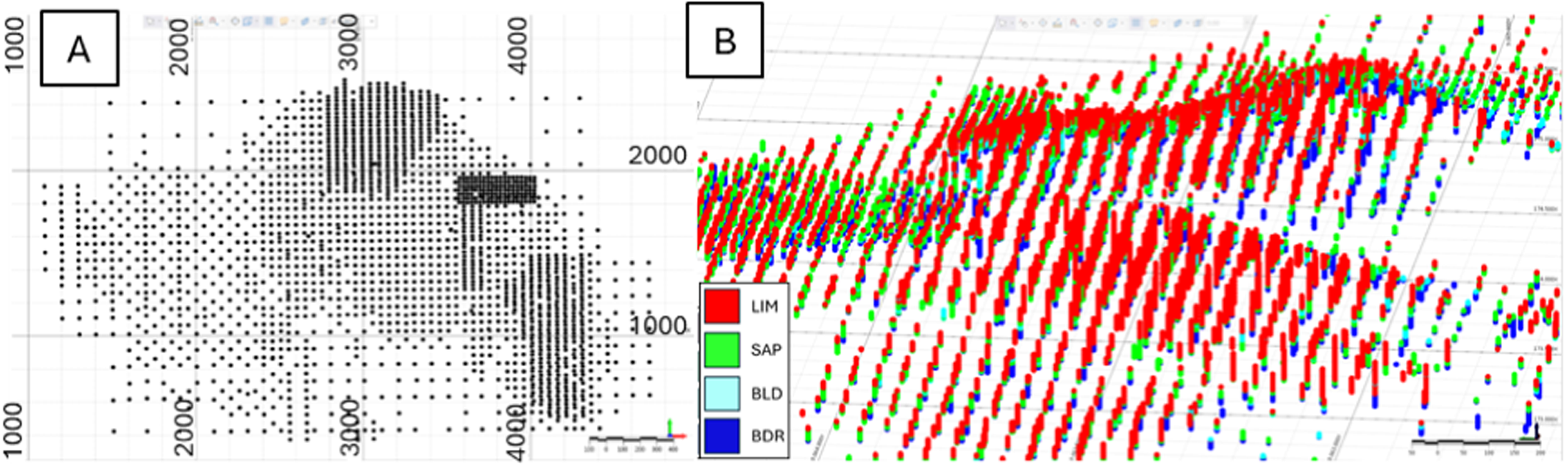
A total of 2217 drillholes with 76,612 composite intervals were used in this study. The layer flagging resulted in 33,626 composite intervals as Limonite, 17,285 as Saprolite, 3854 as Boulder and 10,856 as Bedrock. The data distribution is presented in Figure 2.
Weathering surfaces
The coded database was used to identify the top contact points of each weathering layer. In the database spreadsheet, a formula was created to flag the intervals corresponding to contacts between layers, generating 5624 points for top LIM, 5904 points for top SAP and 3831 points for BDR. Since the top contact of the LIM layer is the best constrained geologically, the surfaces were generated sequentially from top to bottom: Top LIM → Top SAP → Top BDR. These contact points were then used to generate surfaces using radial basis function (RBF) modelling, a method widely applied to the interpolation and reconstruction of irregularly distributed 3D data (Carr et al., 2001).
To avoid interference between layers in areas with limited data support, an offset correction was applied from top to bottom, thereby preserving the original weathering stratigraphy (Figure 3).
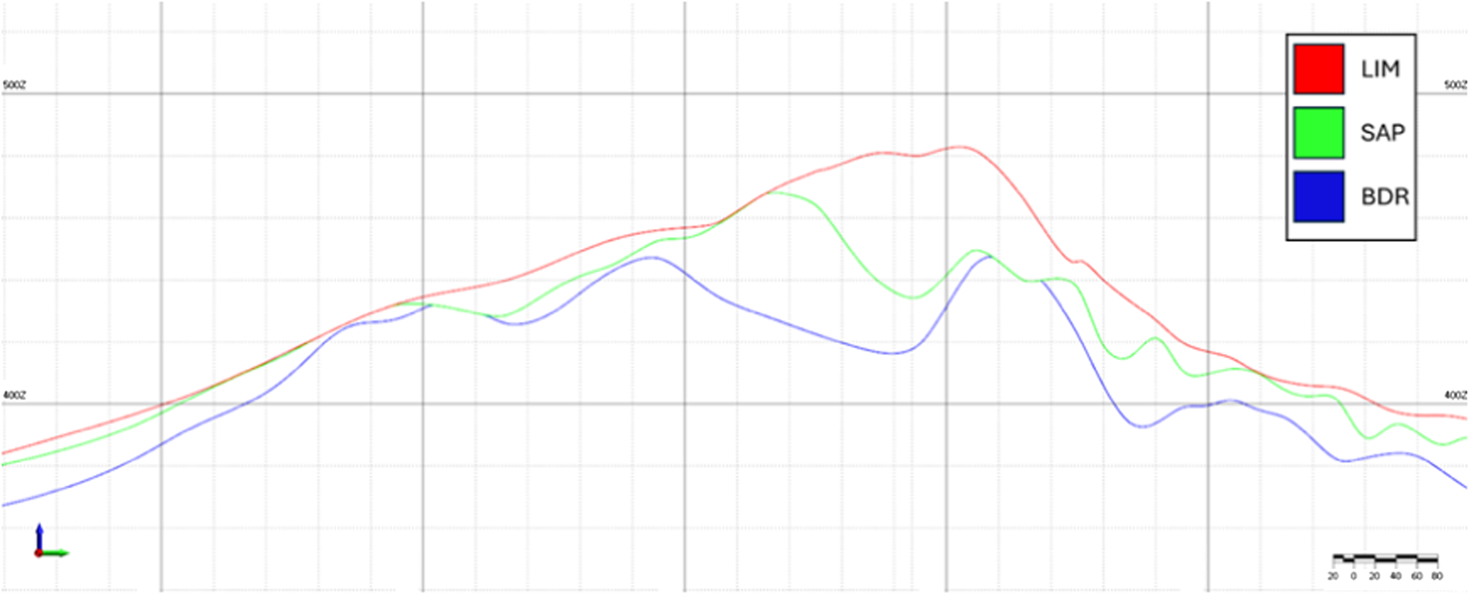
Vertical section exhibiting the contact between the layers, respecting the original weathering profile.
Level of reference and layer variability
In layered weathering profiles, the geometry of geological contacts commonly follows undulating surfaces rather than horizontal stratification, which may obscure the true vertical organisation of the domains when analysed in the original coordinate system. This effect is particularly relevant in lateritic deposits, where weathering fronts may vary significantly in elevation across the deposit while still preserving a consistent relative sequence of materials. The deposit presents significant topographic relief, resulting in a wide range of composite elevations across the study area. The deposit exhibits significant horizontal and vertical variability, as demonstrated by a twin-drilling campaign. The campaign presents four pairs of twinned reverse circulation (RC) and diamond drillholes (DD):
Section 1: RC and DD pair, offset by 2.27 m Section 2: RC and DD pair, offset by 3.00 m Section 3: RC and DD pair, offset by 2.10 m Section 4: RC and DD pair, offset by 1.85 m
A summary of the twin-drilling results, including representative comparison sections, is presented in Figure 4. The comparison of logged material types indicates that Sections 1, 2 and 3 show reasonably consistent geological profiles, although localised grade displacements occur over short distances. The figure highlights the strong natural geological variability at BSD and illustrates the difficulty of obtaining consistently representative twin-drilling results, even at offsets of <3.0 m.
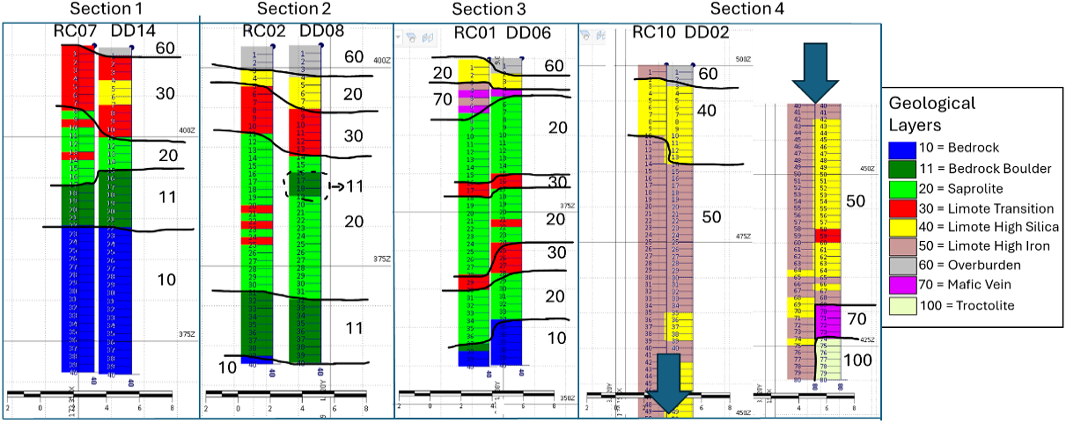
Twin-drilling campaign results exhibiting a comparison of geological layers.
Level of reference and layer variability
Under such conditions, direct statistical analysis of categorical data in Cartesian space may mix different stratigraphic positions and reduce the apparent continuity of the weathering layers. A geometric transformation is therefore required to reposition the data into a stratigraphically consistent framework, in which the relative vertical relationships between layers are preserved, and lateral distortions are minimised.
Because the main directions of lithological continuity are not necessarily horizontal and may vary spatially due to deformation, stochastic modelling should not be carried out directly in the original coordinate system. Instead, a reference horizon can be identified from borehole and structural information and interpolated across the deposit, allowing the domain to be geometrically transformed into a deformed space that restores its probable original configuration. In this transformed framework, variogram analysis and conditional PGS can be performed more consistently, after which the results may be back-transformed to the present coordinate system (Mariethoz et al., 2009).
The definition of a reference level for unfolding in lateritic deposits is inherently more complex than in stratified geological settings, as weathering contacts do not correspond to original depositional surfaces and their geometry is governed by pre-existing topography and protolith structure. The LIM and BDR boundaries were selected as anchoring surfaces because they represent the most geologically consistent and data-supported contacts within the weathering profile.
Therefore, the unfolding method was applied to constrain vertical variability and enable the application of PGS, as the unfolded composites show improved continuity within the geological domains, as demonstrated in Figures 5 and 6 and respective parameters are given in Table 1.
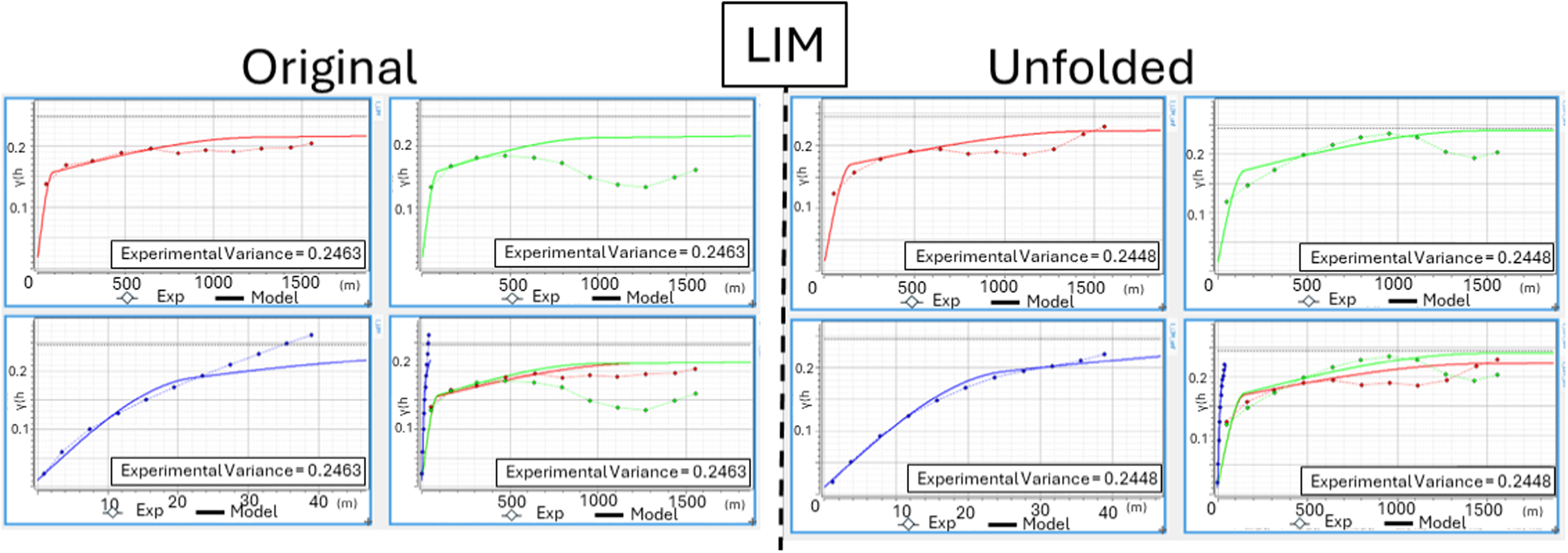
Category indicator variograms for limonite (LIM) category from the original and unfolded composites.
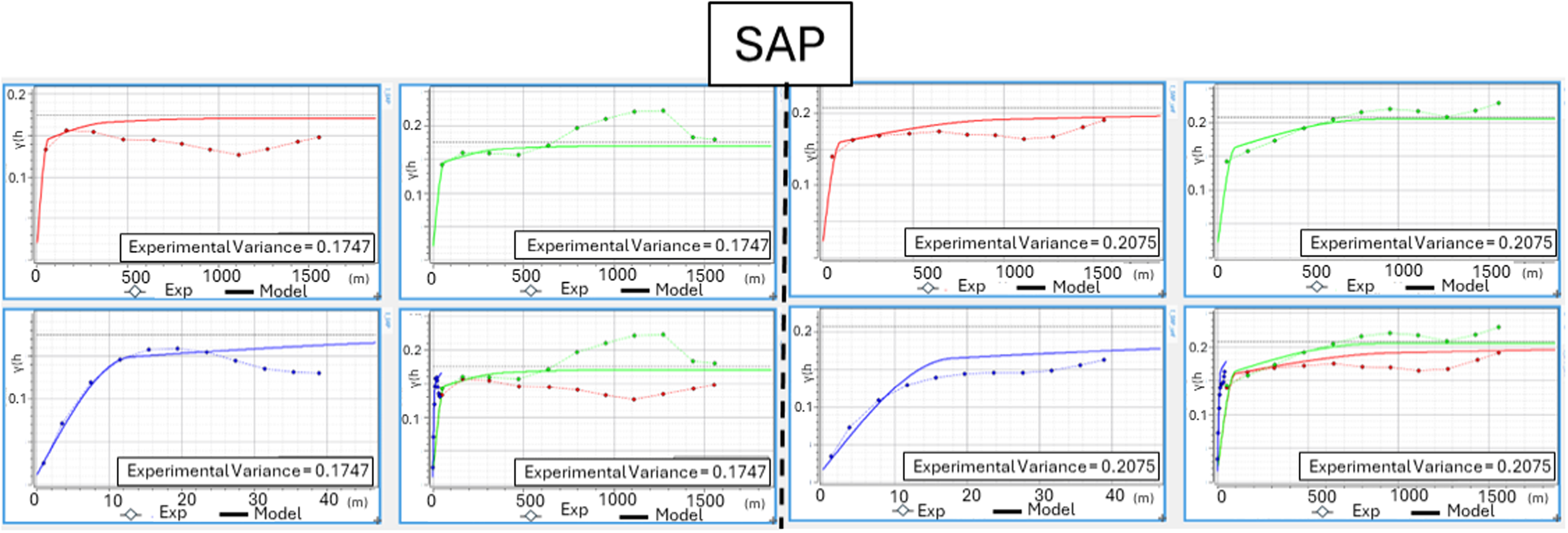
Category indicator variograms for saprolite (SAP) category from the original and unfolded composites.
Variography parameters for categorical indicators.
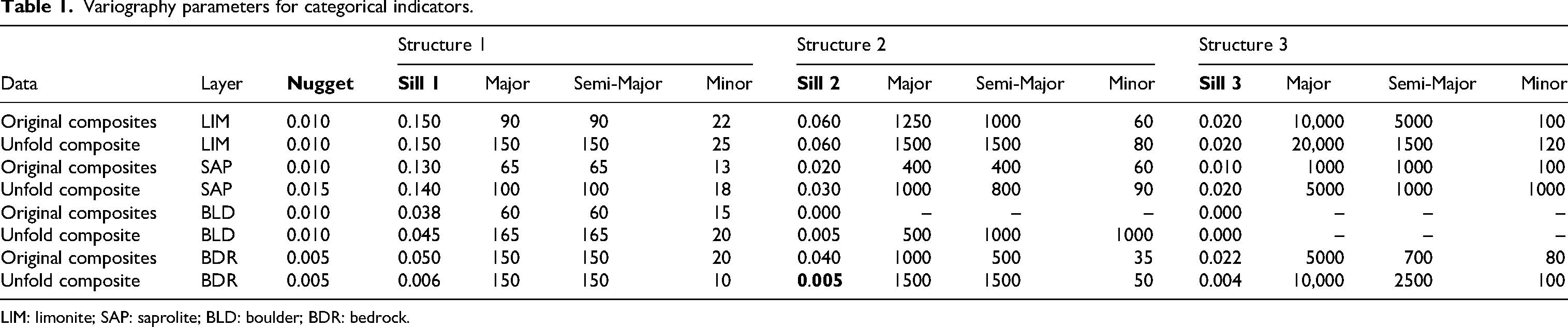
LIM: limonite; SAP: saprolite; BLD: boulder; BDR: bedrock.
Table 1 indicates that the unfolding procedure improved the spatial continuity of the category indicators, particularly for the LIM and SAP layers. In both cases, the variographic ranges increased after unfolding, especially in the short- and medium-range structures, indicating a more continuous and geologically coherent spatial organisation. This effect is particularly evident in the vertical direction, where the increase in range suggests that the unfolding reduced the influence of topographic and geomorphological distortions and repositioned the data into a more stratigraphically consistent framework. As a result, the unfolded composites more accurately reflect the relative continuity of the weathering profile, providing a more suitable basis for VPC modelling and PGS.
Vertical proportion curves
Considering the high variability observed across the deposit and the significant variation in the absolute elevation of the weathering surface contacts, the use of VPCs is justified. VPC is a function that describes the vertical variation in the proportion of categorical domains within a stratigraphic or weathering profile. It expresses the relative frequency of each lithology, facies or weathering unit at successive vertical positions, thereby allowing vertical non-stationarity to be represented explicitly rather than assuming constant proportions throughout the model (Assis, 2024). Within the PGS framework, VPCs are a key component because they define the local categorical proportions to adjust truncation thresholds as a function of depth or stratigraphic position (Armstrong et al., 2011).
After unfolding the data into a stratigraphically consistent framework, VPCs provide an appropriate way to quantify the vertical proportion of each layer and to incorporate this non-stationary behaviour into the PGS through depth-dependent truncation thresholds. This makes them particularly suitable for modelling weathering profiles in which categorical proportions are controlled more strongly by relative vertical position than by absolute elevation.
Unfolding validation was conducted through the comparison between the original composite data VPC and the unfolded composite data VPC (Figure 7).
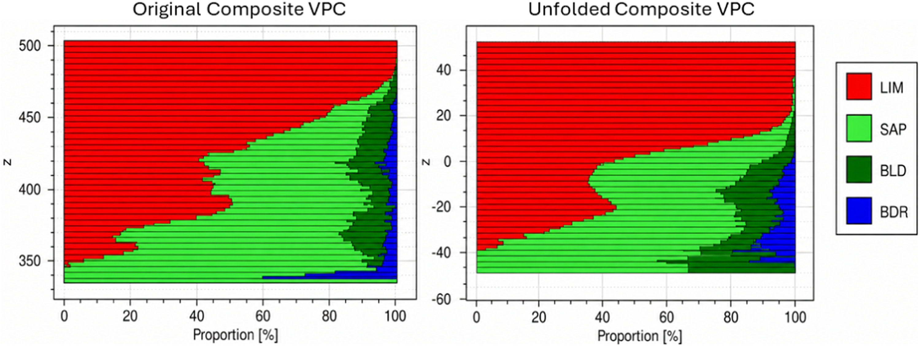
Results of vertical proportion curves (VPCs) for the original composite and the unfolded composite.
Plurigaussian simulation
PGS is a geostatistical approach for modelling categorical variables such as facies or lithotypes by simulating one or more standard Gaussian random functions over the domain of interest and then assigning each category according to the simulated values at each location through a truncation rule. In its simplest form, a single Gaussian field may suffice when the categories follow a clear sequential order; however, more complex geological settings with intricate contacts require two or more Gaussian fields and a rock-type rule to represent the spatial relationships among domains. The method involves selecting an appropriate model type, estimating the relevant parameters, generating Gaussian values at sample locations that are consistent with the observed lithotypes, and finally performing conditional simulation over the grid, after which the simulated Gaussian values are converted back into categorical domains (Armstrong et al., 2011).
The truncation rule is the key parameter in truncated Gaussian methodologies because it controls how geological contacts are represented in the model and governs the conversion of simulated Gaussian values in continuous space into categorical domains. In practical terms, categories adjacent in the truncation rule also tend to be in contact in simulated realisations, making the rule the main mechanism for directly incorporating geological knowledge into the simulation (Assis, 2024).
The truncation rule was defined based on the well-constrained geological relationships observed in the BSD weathering profile (Figure 8). The LIM layer consistently occupies the upper part of the profile and is in direct contact with SAP and, locally, with BLD, reflecting the natural transition from ferruginous and siliceous weathering products into the underlying saprolitic and boulder-bearing horizons. SAP and BLD represent bottom weathering domains and are both observed to overlie BDR, which corresponds to the fresh or weakly weathered serpentinite at the base of the profile. Because these contacts are geologically well-established and follow a vertically organised lateritic succession, the truncation rule was constructed to preserve this relative arrangement, ensuring that the simulated categories reproduce the observed stratigraphic order and the permissible contacts between weathering domains.
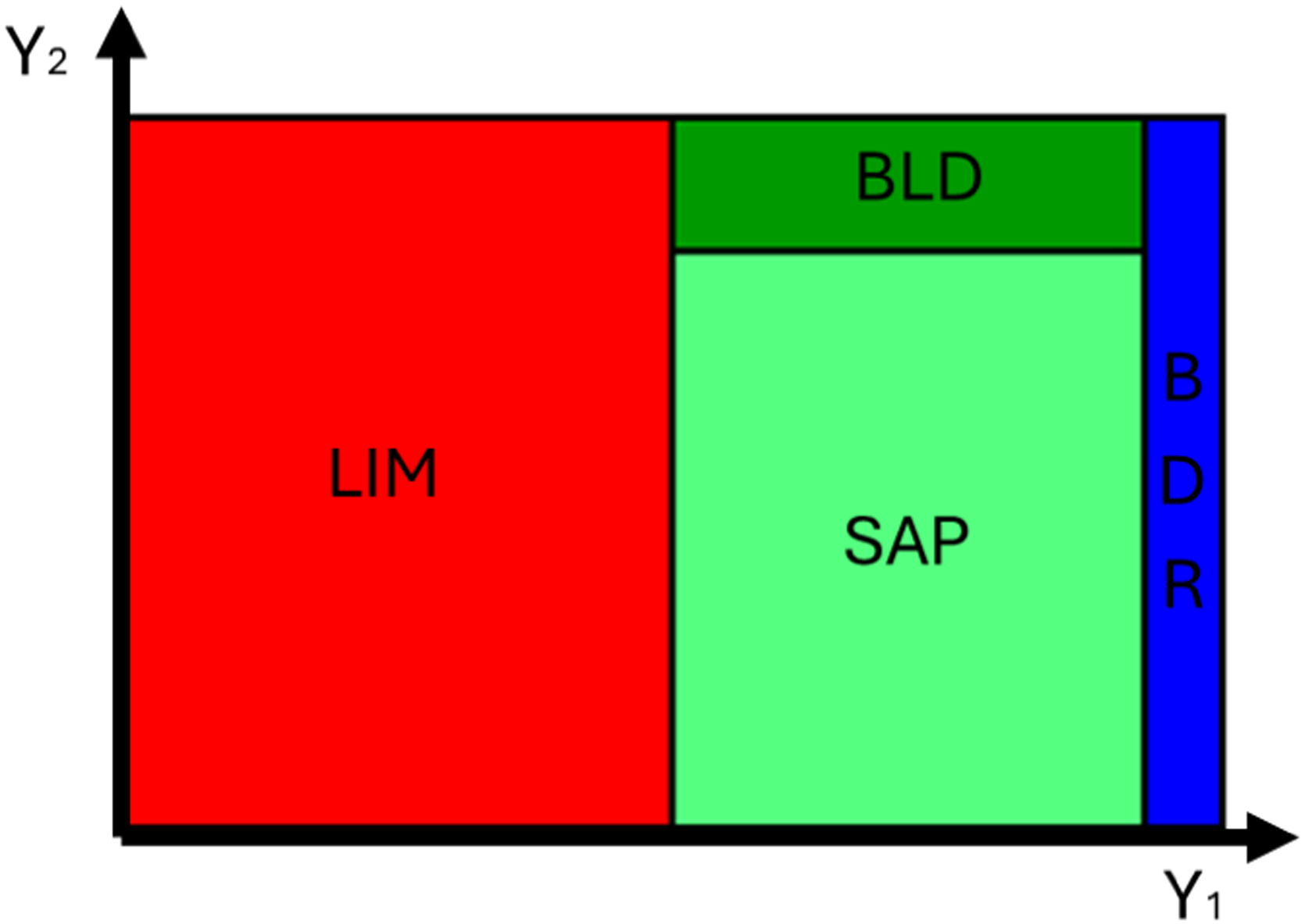
Lithotype rule generated for Brejo Seco Deposit (BSD).
The PGS generated 10 equiprobable realisations for BSD. Due to the large number of grid nodes, the size of the deposit, and the computational resources and time available for the work, a broader sensitivity analysis using a larger number of realisations and Gibbs sampler iterations was not carried out. Based on these realisations, the most probable layer was assigned to each node, corresponding to the lithological class with the highest occurrence frequency at that node across the simulations (Figure 9). In addition, the node-based probability of occurrence for each layer was calculated, providing a quantitative measure of local geological uncertainty and spatial variability in the weathering profile.
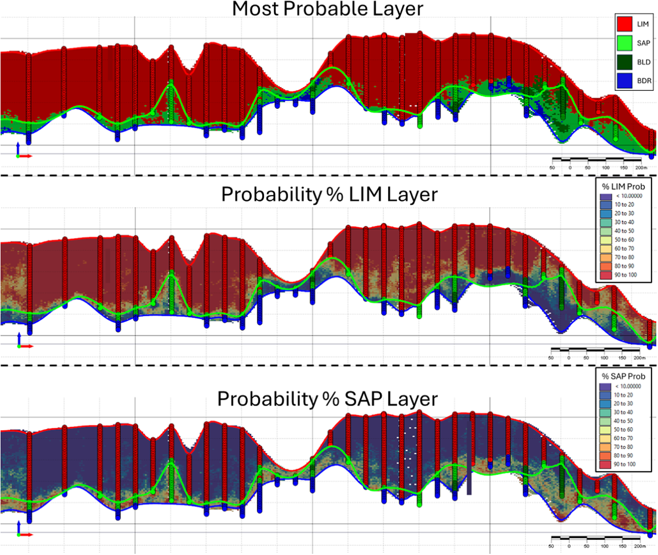
Vertical section illustrating the results of the plurigaussian simulation, including the simulated block model and drillhole composites. The red, green and blue lines represent the top surfaces of the limonite, saprolite and bedrock horizons, respectively.
Results
Risk map
To ensure that the block model support was appropriate for this analysis, the original grid was reblocked to 25 × 25 × 1 m. Two accumulated variables were then generated for each X–Y location to produce 2D risk maps for the limonite layer. The first variable was defined on a node-by-node basis using a probability threshold: nodes were assigned a value of 1 if the simulated probability of belonging to LIM was greater than or equal to 70%, and 0 otherwise. The second variable was derived from the most probable category: nodes were assigned a value of 1 when LIM was the most probable layer and 0 when another category was dominant. In both cases, the accumulated count was normalised by the total thickness at each X–Y location, allowing the accumulated proportion of LIM along the vertical column at each X–Y to be expressed as a percentage. For example, if a given X–Y location contains 10 nodes and nine of them are classified as LIM, the resulting proportion is 90%, indicating a high level of agreement between the simulation outcomes and the deterministic limonite interpretation. This procedure was applied specifically to the limonite layer to identify areas where the deterministic model is more robust and where its accuracy is potentially at risk.
The accumulated 2D risk maps (Figure 10) clearly identified sectors with lower support for the deterministic LIM interpretation. While the central portions of the deposit generally show stronger agreement with the deterministic model, peripheral and locally discontinuous sectors display lower simulated LIM proportions, indicating greater uncertainty in layer continuity and a higher risk of contact misplacement.
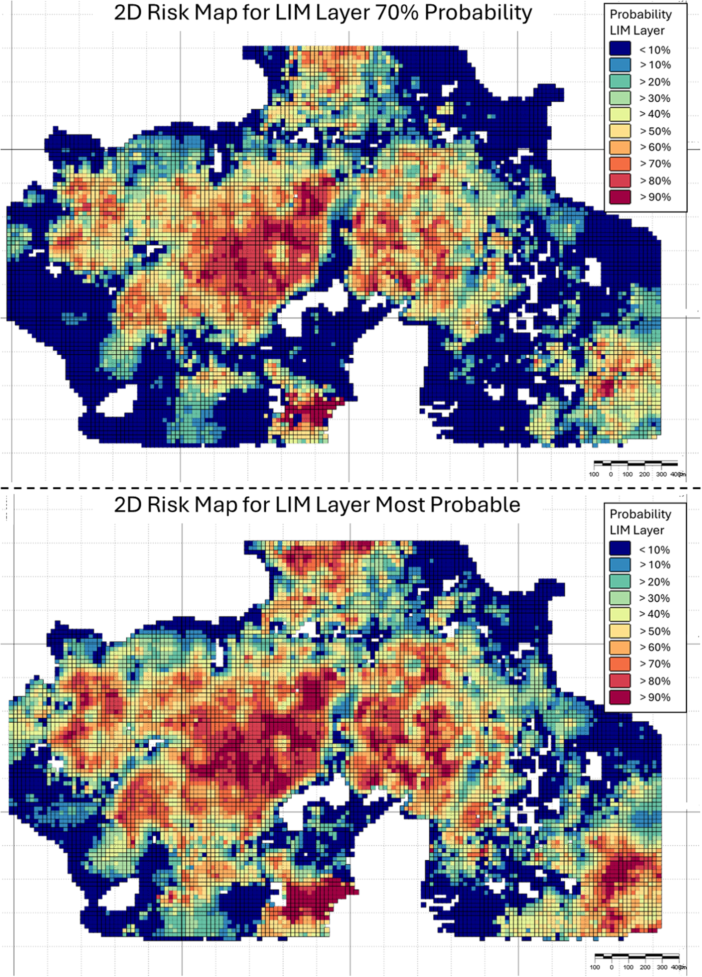
Two-dimensional (2D) accumulated risk maps for the limonite (LIM) layer. The upper map shows the proportion of nodes in each X–Y location with a simulated LIM probability ≥70%, whereas the lower map shows the proportion of nodes in which LIM is the most probable category.
Dilution volume calculation
The potential dilution tonnage within the limonite layer was estimated for each X–Y location using a bulk density of 1.8 g/cm3. This calculation was based on the accumulated 2D variables derived from the simulation results and was performed for both classification criteria: the most probable category and the 70% probability threshold. In this way, areas where the deterministic limonite model is less consistently supported by the simulations could be translated into an estimated tonnage potentially affected by dilution during mining. The estimated dilution tonnage evidenced in Figure 11 highlights the operational significance of the simulated uncertainty. Although large portions of the LIM layer show relatively low dilution potential, specific sectors reach values of up to 90,000 t, indicating that uncertainty in the deterministic contact model may result in significant ore loss or waste contamination if these areas are mined without additional control measures.
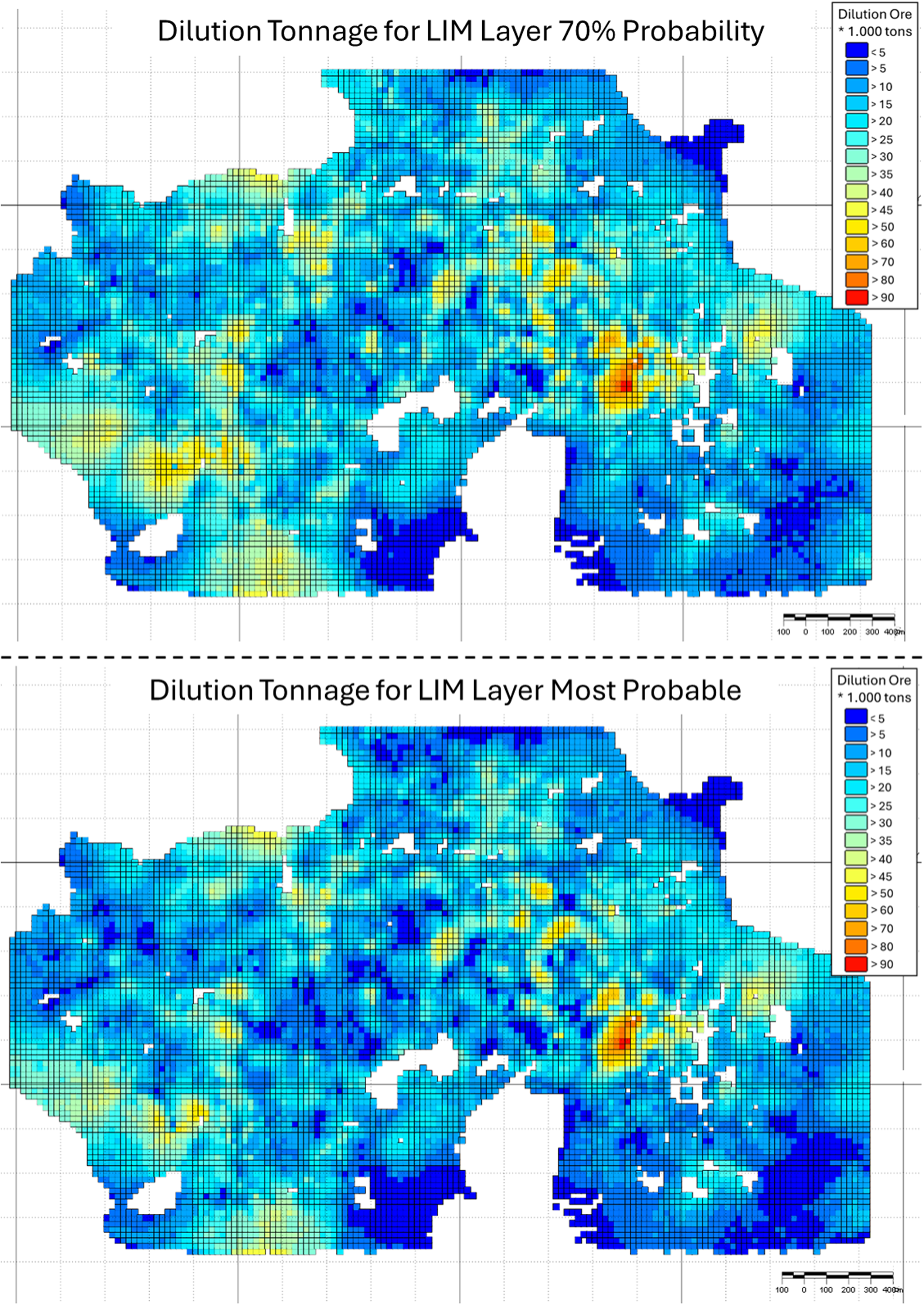
Accumulated dilution tonnage within the limonite (LIM) layer based on the 70% probability threshold (top) and the most probable category (bottom).
Conclusions
Although geological modelling methods have advanced significantly in recent years, the reliability of any geological model remains fundamentally dependent on the quantity, distribution and quality of the available data. In this context, geostatistical simulation provides an effective framework for quantifying uncertainty in model accuracy, particularly in deposits where lithological contacts vary markedly over short distances. The workflow developed in this study integrated unfolding, VPCs and PGS to capture both the vertical organisation and the lateral variability of the BSD weathering profile. The unfolding step proved particularly important, as it improved the spatial continuity of the categorical variables, with increased variographic ranges indicating a more stratigraphically coherent representation of the weathering profile. The results demonstrate that this approach can distinguish areas where the deterministic model is strongly supported from those with a higher probability of misclassification.
This represents an important gain for the geological team, as it, enabling the objective identification of areas of greater uncertainty and supporting decision-making for infill drilling campaigns and future data acquisition. In particular, the accumulated 2D risk maps distinguished sectors where the deterministic LIM interpretation is strongly supported from those where agreement with the simulation results is weaker, thereby highlighting priority areas for model review and geological confirmation.
From a medium- to long-term perspective, the workflow helps constrain lithological contacts that require additional confirmation, thereby improving confidence in the definition of ore and waste volumes. From a short-term mining perspective, the methodology also provides a practical means to quantify local dilution risk, enabling potential ore loss and waste dilution to be anticipated in specific sectors of the deposit. In the LIM horizon, the estimated dilution risk reached up to 90,000 t, demonstrating that local geological uncertainty may translate into a significant operational impact. This is particularly relevant in nickel laterite operations, where selective mining and strict grade control are essential, and where short-range geological variability can directly impact plant feed quality and daily production performance.
The risk products generated in this study included both the most probable category and the probability-threshold approach, using a 70% confidence criterion. The results indicate that the choice of risk metric should be made based on the geological context and operational capacity to incorporate uncertainty into mine planning and process control. In the present case, the most probable category alone is not the most suitable indicator, because a layer may still be classified as dominant even when it has a relatively low absolute probability, especially in a system with four competing categories. For this reason, the probability-threshold approach provides a more robust basis for identifying areas where the deterministic interpretation is insufficiently supported by the simulations.
Future studies should evaluate the uncertainty associated with the reference level used for unfolding in complex weathering profiles, as this may affect the transformed geometry and the subsequent plurigaussian modelling results. Furthermore, although the current PGS parameterisation was considered sufficient for the objectives of this study and for demonstrating the applicability of the proposed workflow to geological control and dilution risk assessment, future work should assess the sensitivity of the results to a larger number of realisations and Gibbs sampler iterations in order to verify whether increased simulation effort materially affects the stability and robustness of the outputs.
Overall, the study shows that the proposed workflow is a practical and effective tool for supporting geological modelling in complex weathering profiles and is therefore considered relevant for geological settings where uncertainty in categorical contacts plays a critical role in resource evaluation and mine planning.
Footnotes
Funding
The authors received no financial support for the research, authorship, and/or publication of this article.
Declaration of conflicting interests
The authors declared no potential conflicts of interest with respect to the research, authorship, and/or publication of this article.