Statistical analysis of earthquake debris extent from wood-frame buildings and its use in road networks in Japan

Abstract

Debris scattering is one of the main causes of road/street blockage after earthquakes in dense urban areas. Therefore, the evaluation of debris scattering is crucial for decision makers and for producing an effective emergency response. In this vein, this article presents the following: (1) statistical data concerning the debris extent of collapsed buildings caused by the 2016 Mw 7.0 Kumamoto earthquake in Japan; (2) an investigation of the factors influencing the extent of debris; (3) probability functions for the debris extent; and (4) applications in the evaluation of road networks. To accomplish these tasks, LiDAR data and aerial photos acquired before and after the mainshock (16 April 2016) were used. This valuable dataset gives us the opportunity to accurately quantify the relationship between the debris extent and the geometrical properties of buildings.

Keywords

LiDAR the 2016 Kumamoto earthquake debris road networks

Introduction

In the aftermath of a large-scale disaster, the delivery of relief is one of the most important tasks for disaster managers. The relief demand must be fulfilled in the shortest possible time. Therefore, the road network condition plays an important role. The blockage of a road network compromises a proper and efficient evacuation of survivors to safe areas. The long-term consequences of road blockage include the disruption of customer access, commuting, and shipping and supply, which greatly affects local businesses and employment.

Information related to the effects of damage on road networks is available. After the Kobe earthquake, Sato et al. (1996) surveyed companies and employees in the four central wards of Kobe to study changes in commuting and working patterns. Out of all the responders, 61.9% and 32.7% cited “no access” and “partial access” to transportation, respectively, after the earthquake. In addition, the main commuting method changed from “train” (with 66.4%) to “on foot” (35.4%). Gordon et al. (1998) performed telephone interview surveys and estimated total business interruption losses of $6.5 billion due to the 1994 Northridge earthquake, of which $1.5 billion were transport-related interruptions. Eshghi and Ahari (2005) reported on the performance of the transportation system in Bam city after the 2003 Bam, Iran earthquake and pointed out that the earthquake did not cause any collapse of main roads or any severe structural damage to bridges. However, the debris caused by the collapse of buildings led to the blockage of some streets and alleys. Scawthorn and Rathje (2006) summarized the effect of the 2004 Niigata-Chuetsu, Japan earthquake. In the study, the total cost of damage was estimated at almost $40 billion, of which the main contribution, $12 billion, was damage to local roads, railways, rivers, and bridges. Maruyama and Itagaki (2017) summarized the report of the Ministry of Land, Infrastructure and Transport related to road network damage by the 2011 Tohoku-oki earthquake tsunami, in which the main damage patterns were roadway cracks, road shoulder collapse, embankment collapse, landslide, joint gaps, and asphalt detachment. Miyagi Prefecture was the most severely affected, with more than 2000 km of road exposed to the tsunami. Roadway cracks and embankment collapses were reported as the main damage patterns. During Hurricane Harvey in 2017, many roads that lead out of the affected areas, such as Houston, were flooded, closed, or damaged due to heavy rainfall (Texas Department of Transportation, 2017).

The Disaster Waste Management Guidelines (UNEP/OCHA, 2011) recommend, as part of the phase 1: emergency phase, cleaning the main streets within the first 72 h to provide access for search and rescue efforts and relief provisions. However, according to the referred guidelines, the disaster waste moved should stay in the emergency area until appropriate disposal sites have been identified, which belongs to the phase 2: early recovery phase. Due to its evident role in emergencies, special attention has been paid to seismic road network analysis. As mentioned before, the causes of damage to road networks are diverse. It was pointed out that the seismic risk assessment of transportation networks in high-dense urban areas mainly depends on the seismic performance of buildings that may interfere network links (Argyroudis et al., 2015; Goretti and Sarli, 2006; Zanini et al., 2017). For instance, The Italian National Seismic Prevention Program assigns the potential interference of accessibility routes in relation to the height of isolated buildings, the height of structural aggregates, and the width of the street/road (Dolce, 2012).

Goretti and Sarli (2006) introduced a methodology to compute the seismic road vulnerability for urban areas, in which the road failure probability, $P_{f}$ , depends on the seismic intensity, I, and the number of building blockages when intensity I affects the road, $N_{b | I}$ . Further development of the methodology requires the characterization of building vulnerability class, T, and probability that a building with vulnerability T will block the road, $P [b | T, I]$ . Moreover, the computation of $P [b | T, I]$ requires the definition of damage grades, d, the causes of road failure, k, and the probabilities $P [d | T, I]$ , $P [k | d, T]$ , and $P [b | k, T]$ . Considering that the parameters T, k, and d are discrete variables, $P [d | T, I]$ and $P [k | d, T]$ are expressed in matrices and are evaluated based on the statistical analysis on Italian post-earthquake surveys. However, such detailed information is often unavailable in other regions.

Argyroudis et al. (2015) pointed out that the debris width produced by a collapsed building that is extended further than the initial building’s boundary, hereafter referred to as debris extent $(D)$ , is required for the road blockage assessment. Because of the complexity and the lack of information, the estimation was based on engineering judgments and assumptions. Thus, four simplified geometrical models of collapsed buildings were defined, each representing a collapse mode. Using such geometrical modes, D is computed as a function of the initial width of the building, W, the inclination angle of the collapsed building, c, the ratio between the volume of the building after collapse and the original volume, $k_{v}$ , and the height of the building, H. An application of the method to Thessaloniki, Greece, was presented in the referred study, from which the following were observed: The available fragility function for collapsed buildings did not consider the collapse mode. Thus, one failure mode was chosen manually for the all study area. The parameter W was assumed constant at 15 m. The parameters c and $k_{v}$ were assumed to follow a normal distribution with means of 45 and 0.5, and coefficients of variation of 30% and 30%, respectively.

Zanini et al. (2017) also pointed out that the quantification of the road area potentially obstructed by the debris is rather complex to be performed from an analytical model. Thus, a fuzzy logic system was employed to evaluate the obstructed road width. The fuzzy model was calibrated from a set of masonry building collapses that occurred in previous earthquakes. In the referred work, the percentage of obstructed road width due to a collapsed building i, $α_{hbi}$ , was proposed as a function of the road width, $W_{rs}$ , and the building height, H. The parameters $α_{hbi}$ and the debris extent, D, provide a similar information in different formats. For instance, for a collapsed building located beside a road and without any building in the other side of the road, $D = α_{hbi} W_{rs}$ if $α_{hbi} < 1$ ; otherwise $D > α_{hbi} W_{rs}$ . Osaragi and Oki (2017) implemented an integrated simulation model of an earthquake-induced damage scenario. In their model, the safest assumption was made for the value of D, that is, the debris extent was considered to be equal to the building height, $D = H$ .

In this article, we aim to improve the estimation of D by performing a precise quantification of the debris produced by the collapsed buildings in the 2016 Mw 7.0 Kumamoto earthquake, Japan. For this purpose, D was quantified using airborne light detection and ranging (LiDAR) technology and aerial photographs. Then, a statistical approach was employed to study the possible correlation between the debris expansion and geometrical features of buildings. Based on the aggregated statistics, probability functions are proposed for the length of D.

The Kumamoto earthquake

On 14 April 2016, an Mw 6.2 earthquake struck Kumamoto Prefecture, Japan, at 21:26 JST (UTC + 9). The epicenter was located at the end of the Hinagu fault at a shallow depth. After approximately 28 h (at 01:25 JST on 16 April 2016), another earthquake of Mw 7.0 struck the same area. The epicenter occurred at the Futagawa fault and near the Hinagu fault (Figure 1). The Futagawa and Hinagu faults are well-known active faults on Kyushu Island, Japan. The first and second events were designated as the foreshock and mainshock, respectively. With 340 aftershocks larger than Mw 3.5 by April 2017, the Kumamoto earthquake is the inland event that has produced the largest number of aftershocks in Japan (Japan Meteorological Agency, 2017). The town of Mashiki, which has a population of approximately 33,000 people, was the most severely affected in terms of buildings, bridges, and lifelines. According to the Cabinet Office of Japan (2017), a total of 8697 houses collapsed and 228 casualties occurred as of 13 April 2017.

Figure 1.

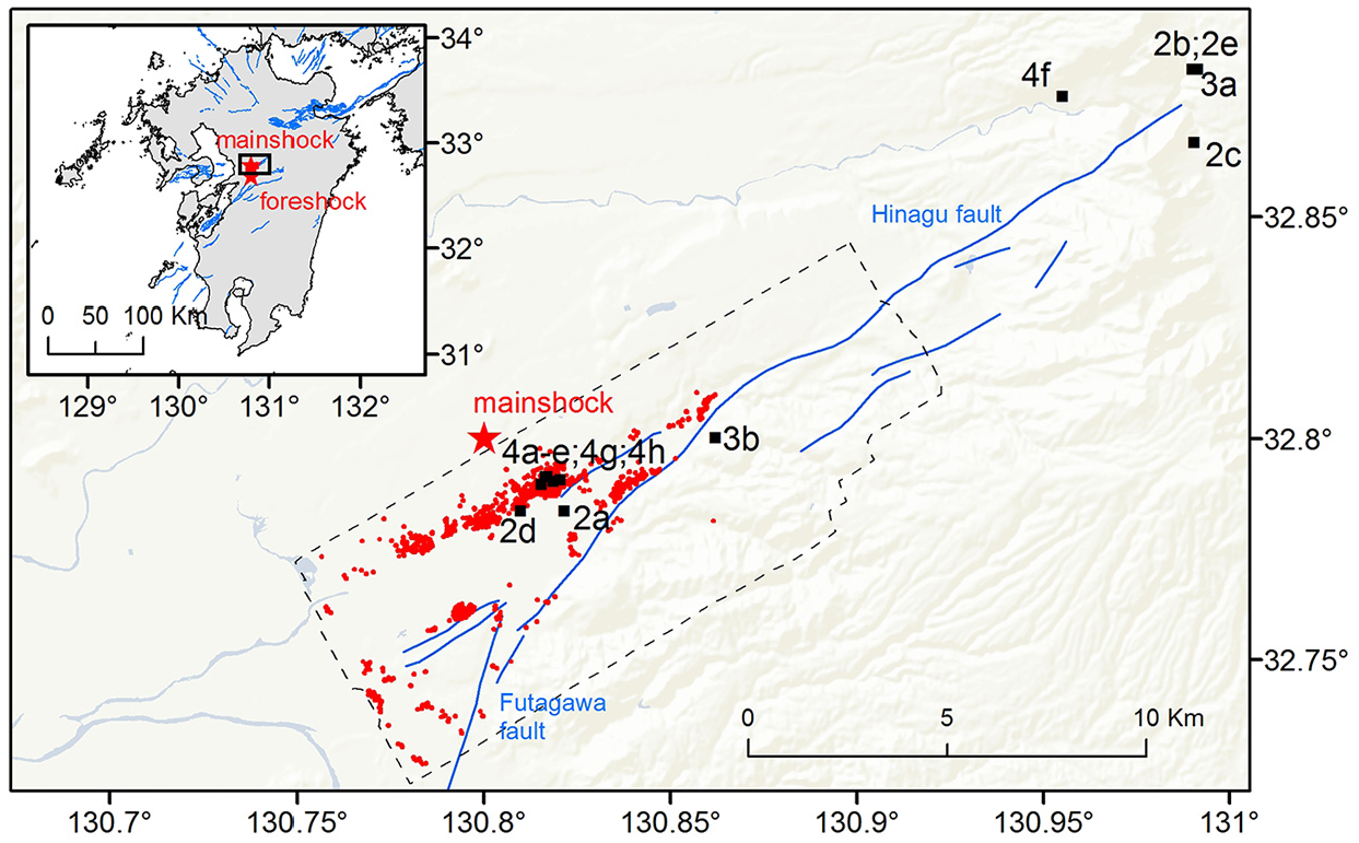
Spatial distribution of collapsed buildings, shown as red marks, used in this study. The inset shows the location of the study area within Kyushu Island, Japan. The red stars show the location of both the foreshock and the mainshock. The dashed line depicts the boundary of the ADSM. The black square marks show the locations of the survey photos shown in Figures 2 to 4.

A series of field investigations, led by the third author, were performed during 15–17 April, 6–7 June, and 3–4 July (Yamazaki and Liu, 2016). Figure 2 shows cases of road damage due to ground failure. Landslide affected the road network as well (Figure 3), and one of the biggest landslides occurred in the Kawayo district in Minami-Aso village. The Aso-Ohashi bridge, which has a span of 206 m and a width of 8 m, fell into the Kurokawa river due to this landslide (Figure 3a). Figure 4 shows the debris produced by collapsed buildings. Note that, during the survey on 3–4 July, most of the debris had already been removed from the roads, but remains in the affected area (Figure 4g and h).

Figure 2.

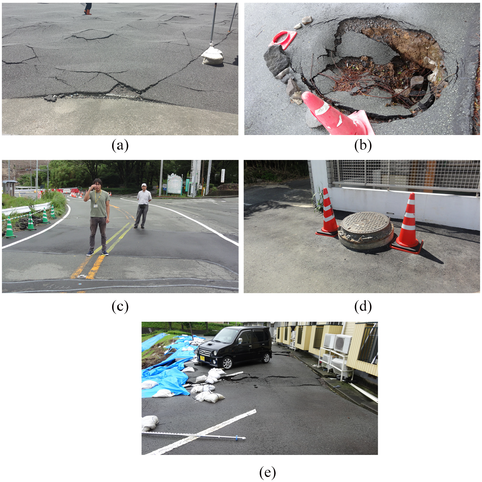
(a-e) Illustrations of ground failure in roads. Photos taken during the survey on 3 July 2016. The locations of the photos are shown in Figure 1.

Figure 3.

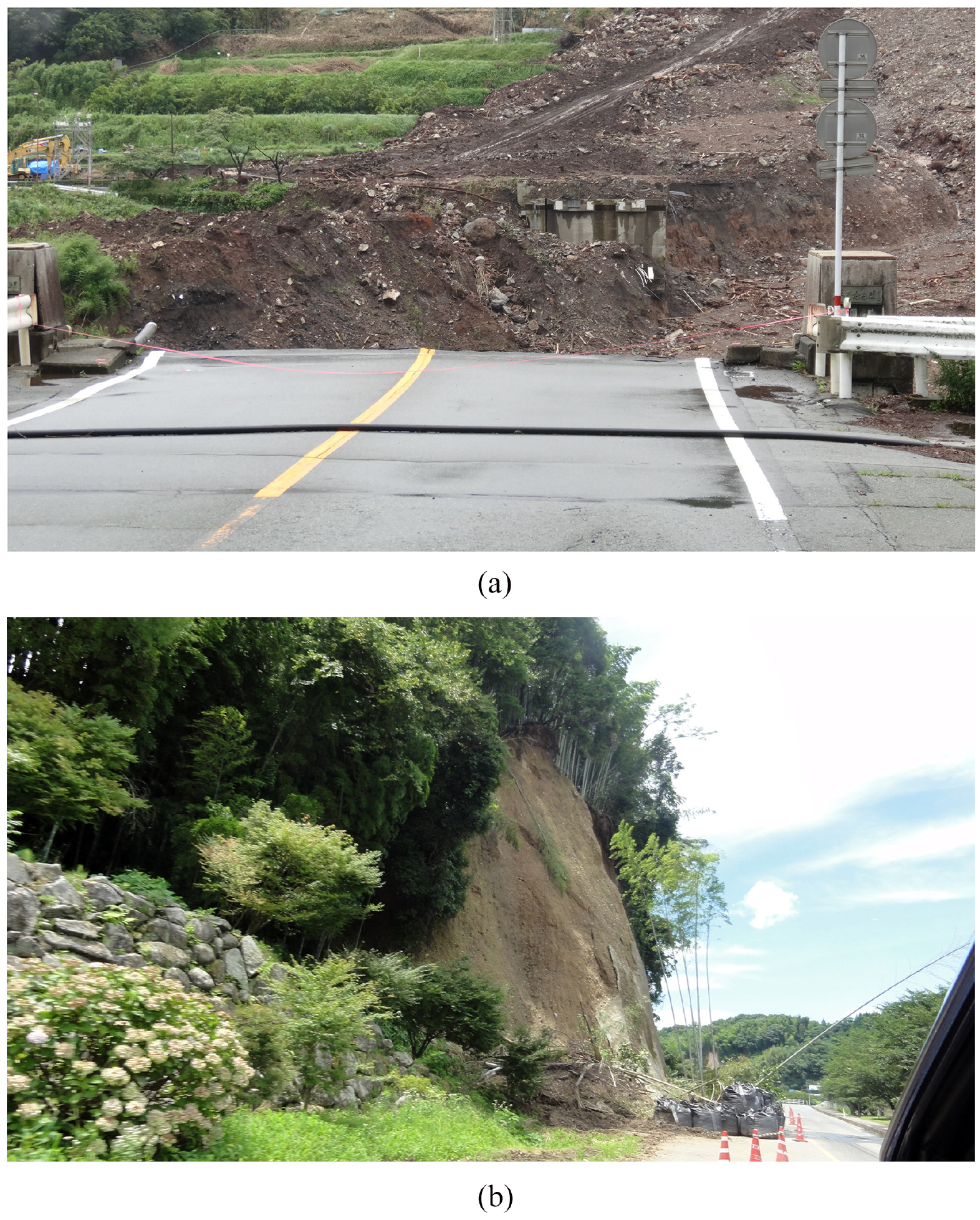
(a) Collapse of a bridge and (b) landslide. Photos taken during the survey on 3 July 2016, and their locations are shown in Figure 1.

Figure 4.

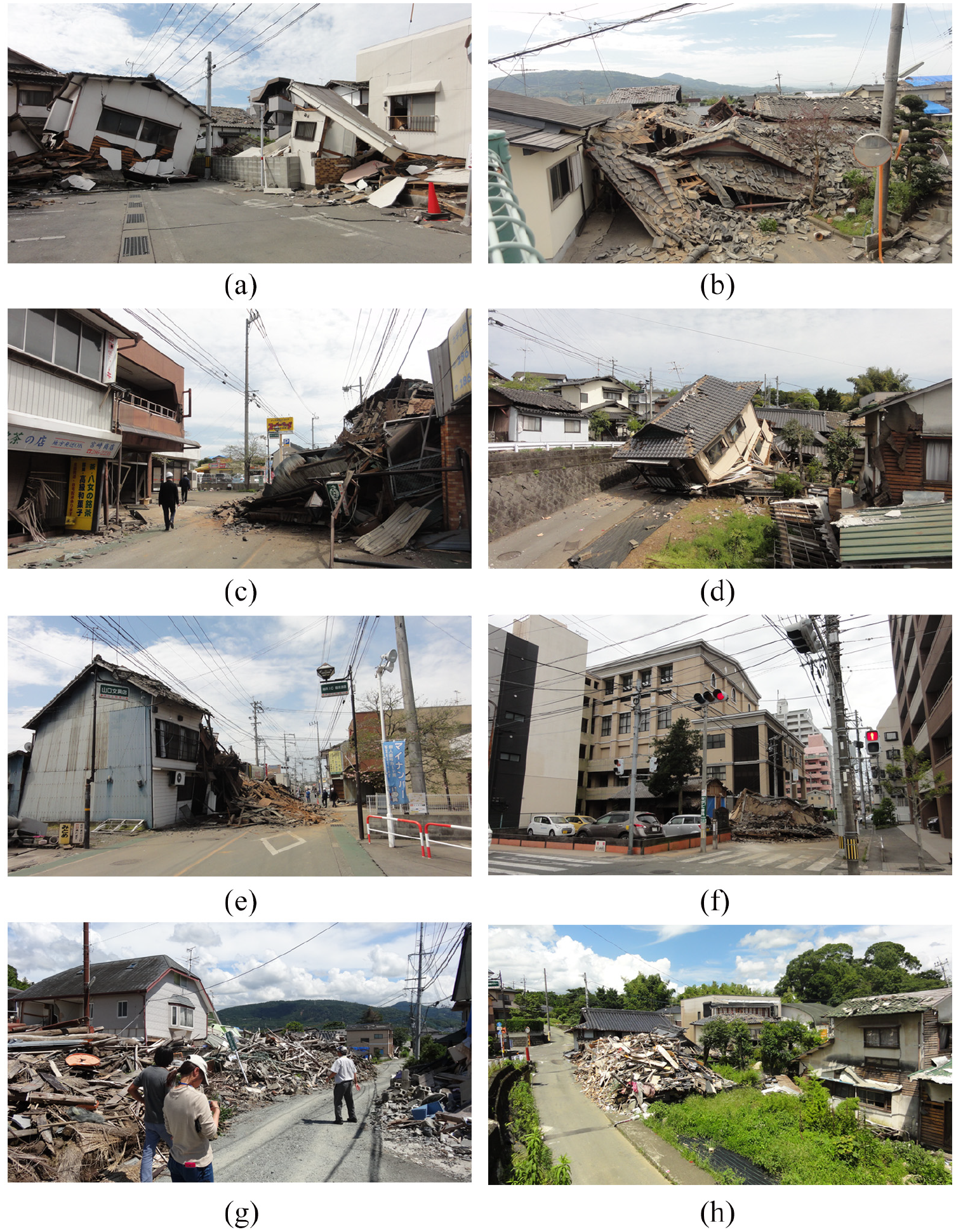
(a–f) Illustrations of roads blocked by collapsed building. Photos were taken during the survey on 15–17 April. (g, h) Photos taken during the survey on 3–4 July. Examples of roads cleaned for accessing purposes. Note that the debris have only been removed from the roads. The locations of the photos are shown in Figure 1.

Database

Different types of remote sensing data were used to monitor the effects of the 2016 Kumamoto earthquake (Liu and Yamazaki, 2017; Moya et al., 2017a, 2017b, 2017c; Yamazaki and Liu, 2016). In this study, the collapsed buildings extracted by Moya et al. (2017b) are used. A building was classified as collapsed if its damage grade was D5 according to the damage pattern chart proposed by Okada and Takai (2000), that is, one or more stories of the building disappeared (Figure 4a to f). The collapsed buildings were extracted from a pair of digital surface models (DSMs) taken before and after the mainshock and a vector database of building footprints. The DSMs were constructed from the LiDAR data. Three features were calculated for each building: (1) the average of the differences in elevation between the two DSMs; (2) the standard deviation of the differences; and (3) the correlation coefficient between the DSMs. These features were calculated within a vector database modified from the building footprints in order to avoid errors in the building boundaries. Using the survey data by Yamada et al. (2017), a threshold to separate collapsed and non-collapsed buildings was calibrated.

Regarding the airborne LiDAR data, the Asia Air Survey Co., Ltd. (2016) sent the first mission to record the affected areas on 15 April 2016, 1 day after the foreshock. A cloud point with a density of 1.5–2 points/m² was obtained. Later, the second mission was set up on 23 April 2016, 7 days after the mainshock. A cloud point density of 3–4 points/m² was achieved at this time. The area of the second mission is located within the area of the first mission. Thus, our study is basically in the area of the second mission, which is shown in Figure 1 as a polygon with a dashed line. The DSMs were obtained after the rasterization of the two LiDAR datasets. From now on, BDSM and ADSM will refer to the DSM obtained before and after the mainshock, respectively. Both DSMs have a data spacing of 50 cm and are registered in the Japan Plane Rectangular Coordinate System.

Moya et al. (2017b) performed an automatic procedure to extract collapsed building, and although a high accuracy was achieved, there were misclassifications in their results. An automatic procedure to extract damaged regions right after a natural disaster is very important for producing a quick response and recovery. For a quick response, there is mostly a trade-off between automation and accuracy. However, our purpose here is to precisely quantify D caused by collapsed buildings. Thus, a first filter was performed before the quantification of D. The following buildings were removed from the collapsed building database:

Misclassified collapsed buildings. These refer to non-collapsed buildings classified as collapsed during the automatic classification performed by Moya et al. (2017b). Furthermore, during the automatic classification, some buildings that had already collapsed during the foreshock were also extracted due to the perturbation of their debris during the strong ground motion of the mainshock. Those buildings were removed as well because it was not possible to quantify their debris using the procedure explained in the next section.

Collapsed buildings obstructed by neighboring buildings. The reason for this decision was that the natural pattern of debris expansion was probably affected by the neighboring buildings (Figure 5c and d). Therefore, more bias would be introduced rather than making a meaningful contribution to the aggregate statistics.

Collapsed buildings for which debris was not quantifiable. The affected area has patches of grass, plants, and trees, and thus, in several cases, these features hide the debris produced by collapsed buildings (Figure 5b). Therefore, it was decided not to include these buildings.

Figure 5.

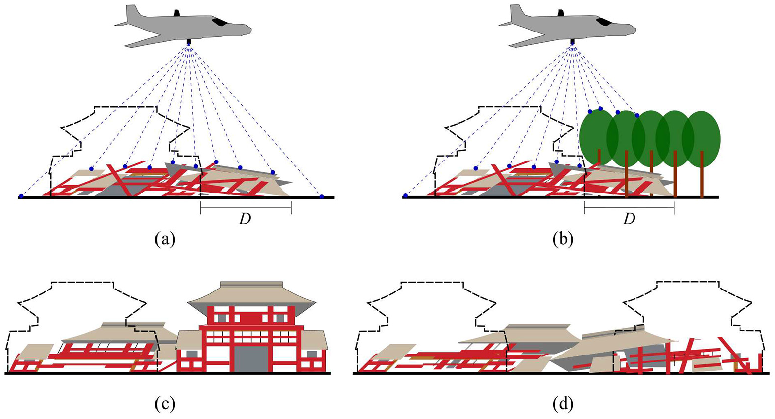
Scheme of the selection of samples. (a) The debris spread toward a free area, and thus it was used for the statistical analysis. (b) The debris spread toward a highly dense vegetation area, in which LiDAR did not reach the debris. (c) The debris spread was disrupted by a neighbor building. (d) The debris spread was mixed with debris from other collapsed buildings. Samples of the type (b), (c), or (d) were neglected for the statistical analysis.

This first screening was performed by visual inspection using the DSMs and the aerial photos. After filtering the types of buildings mentioned above, a total of 1099 buildings were selected (Figure 5a). The spatial distributions of the selected buildings are shown in Figure 1. The selected buildings are mainly located in Mashiki town and parts of Kumamoto city, Kashima and Mifune towns. The next issue to address was the improvement of the vector database of building footprints used in Moya et al. (2017b). The building footprint vector dataset was provided by the Geospatial Information Authority of Japan (GSI). Figure 6a shows a close-up of the BDSM where the vector data of a building footprint can be observed. There is not a perfect match between these two datasets. Therefore, another preprocessing step was required: First, the vector data were rasterized (Figure 6b) and then shifted iteratively around the center in order to evaluate the level of matching with the BDSM. The level of matching was estimated using the correlation coefficient. Figure 6c shows the correlation coefficient calculated from different shifts of the footprint. Here, the location of the largest value with respect to the center of the image represents the distance that must be applied to the building footprint in order to match the BDSM (Figure 6d). This automatic procedure was applied to the selected buildings. The results were verified by visual inspection and were corrected if necessary.

Figure 6.

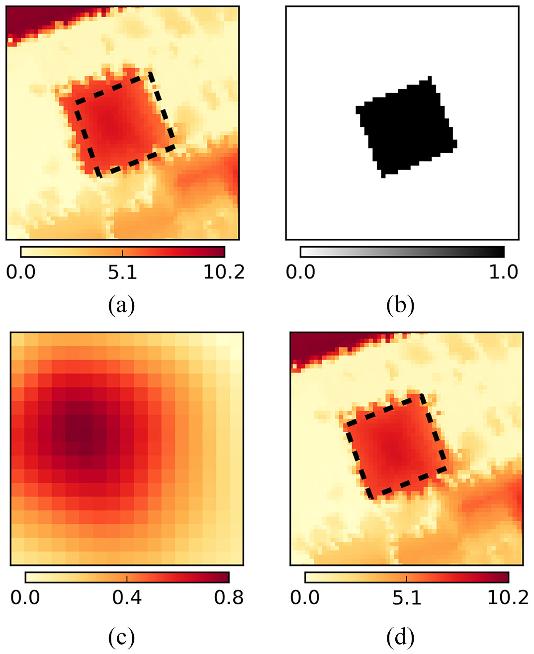
(a) BDSM and original footprint of a collapsed building; (b) raster presentation of the original building footprint; (c) correlation coefficient between the BDSM and building footprint shifted in several directions; (d) BDSM and updated building footprint. The color bars in (a) and (d) show the elevation in meters.

Debris extent of collapsed buildings

The length of D was quantified from the DSMs (Figure 5a). Figure 7a and b shows the BDSM and ADSM, respectively, of the same building shown previously. After the mainshock, it is observed that the building has collapsed to southwest. The DSMs give the opportunity to measure the debris extent with a high precision, which has not been done before. However, the use of LiDAR to measure the volume of debris in roadways has been reported elsewhere (Axel et al., 2016). The LiDAR data show clear advantages compared to the aerial photos. Although the spatial resolution is lower than the aerial photos, the precision in elevation is at the centimeter level, which is crucial in detecting debris. In addition, aerial images contain geometric distortions, and thus using these images to quantify the debris expansion would introduce some errors. Figure 7c shows the differences in elevation between both DSMs. Here, the highest values depict the direction to which the debris has spread, and the lowest value shows the opposite side. In order to extract the debris, an image threshold was applied in which differences in elevation greater than or equal to 50 cm are set equal to 1; otherwise, these values are set to 0. Figure 7d shows the debris distribution.

Figure 7.

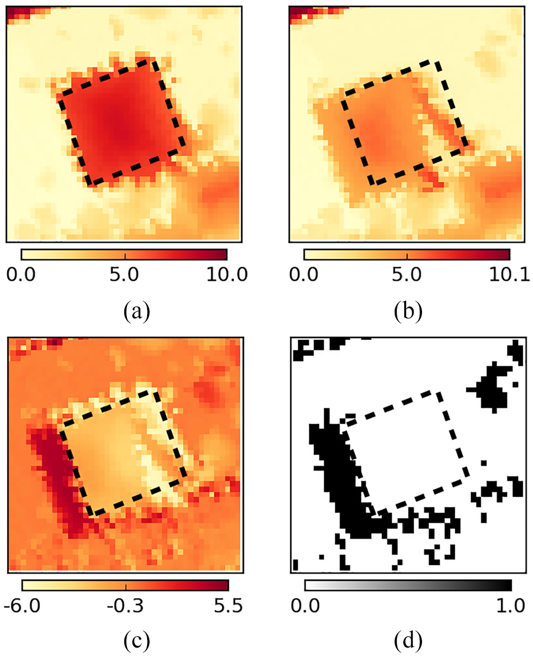
(a) BDSM and updated building footprint; (b) ADSM and updated building footprint; (c) difference between the DSMs (ADSM – BDSM); (d) binary image where a pixel is set to 0 if the difference between both DSMs is less than 50 cm; otherwise, the pixel is set to 1 ((ADSM – BDSM) ≥ 0.5 m). The units of the color bars in (a) to (c) are in meters.

For the quantification of D, polygons parallel to the footprint at distance intervals of 50 cm were drawn. Profiles such as that shown in Figure 8 were prepared for each building. Although not shown in Figure 8, parallel polygons until a distance of 9.5 m were drawn. For ease of visualization, the debris outside the polygons was removed. It is now clear that the debris extent was 3.5 m for this sample building. The length of D for the 1099 buildings was measured manually with the aid of these profiles. Then, a second filter was applied at this stage. The number of reinforced concrete and steel buildings within the study area was small, and thus a statistical analysis was not possible. Therefore, concrete and steel buildings were removed from the analysis. Finally, 851 wooden buildings were selected for further analysis.

Figure 8.

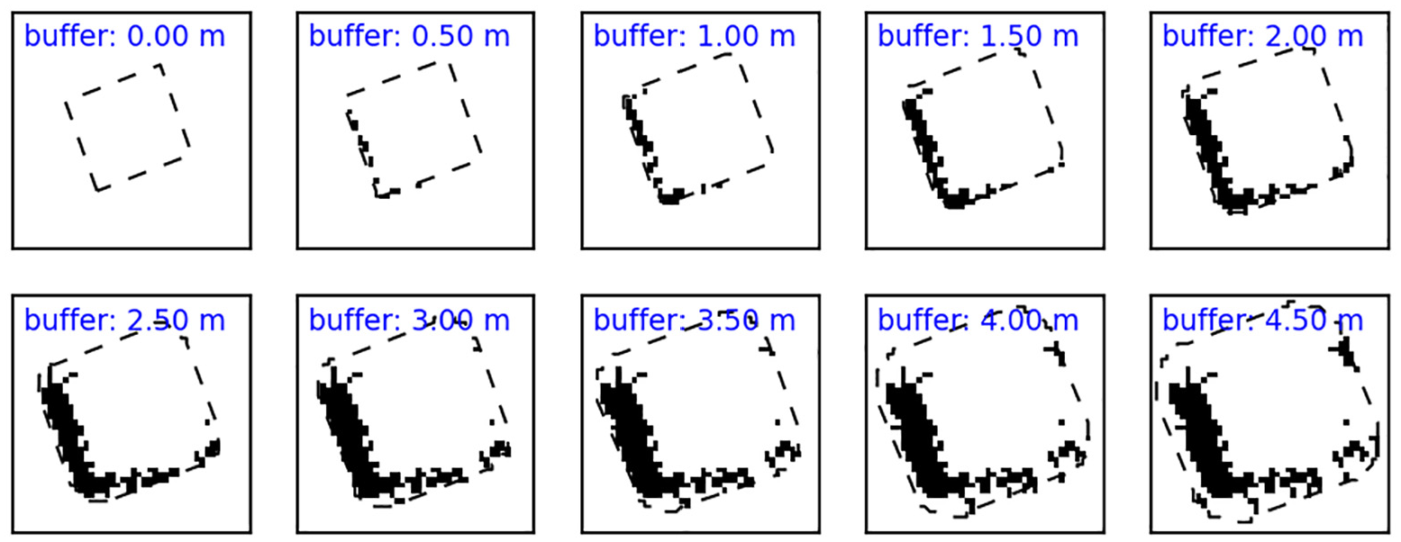
Polygons parallel to the building footprint and separated by distances at intervals of 50 cm. The spatial distribution of debris within the polygons is also shown.

Figure 9 shows the scatter plots of D with respect to a few geometrical features of buildings. Each mark represents a measurement for one building. As can be observed, D was measured in intervals of 50 cm. In order to visualize where the samples are clustering, the color mark depicts the point density of samples with an equal value of D. The density was estimated using Gaussian kernels (Scott, 1992). The scatter plots show the absence of linear correlation between D and the building footprint area (Figure 9a) and the building aspect ratio (Figure 9b). The building aspect ratio was calculated as the ratio between the lengths of the shortest and longest sides of a building footprint. Building height $(H)$ , however, shows a moderate correlation with D (Figure 9c). This observation was expected because previous studies used building height as the major parameter. For instance, in the conservative estimation proposed by Osaragi and Oki (2017), an equation to calculate the debris height $h'$ at a given distance from the building boundary w was presented:

h' = (0.32 H + 0.853) (1 - \frac{w}{H}) .

(1)

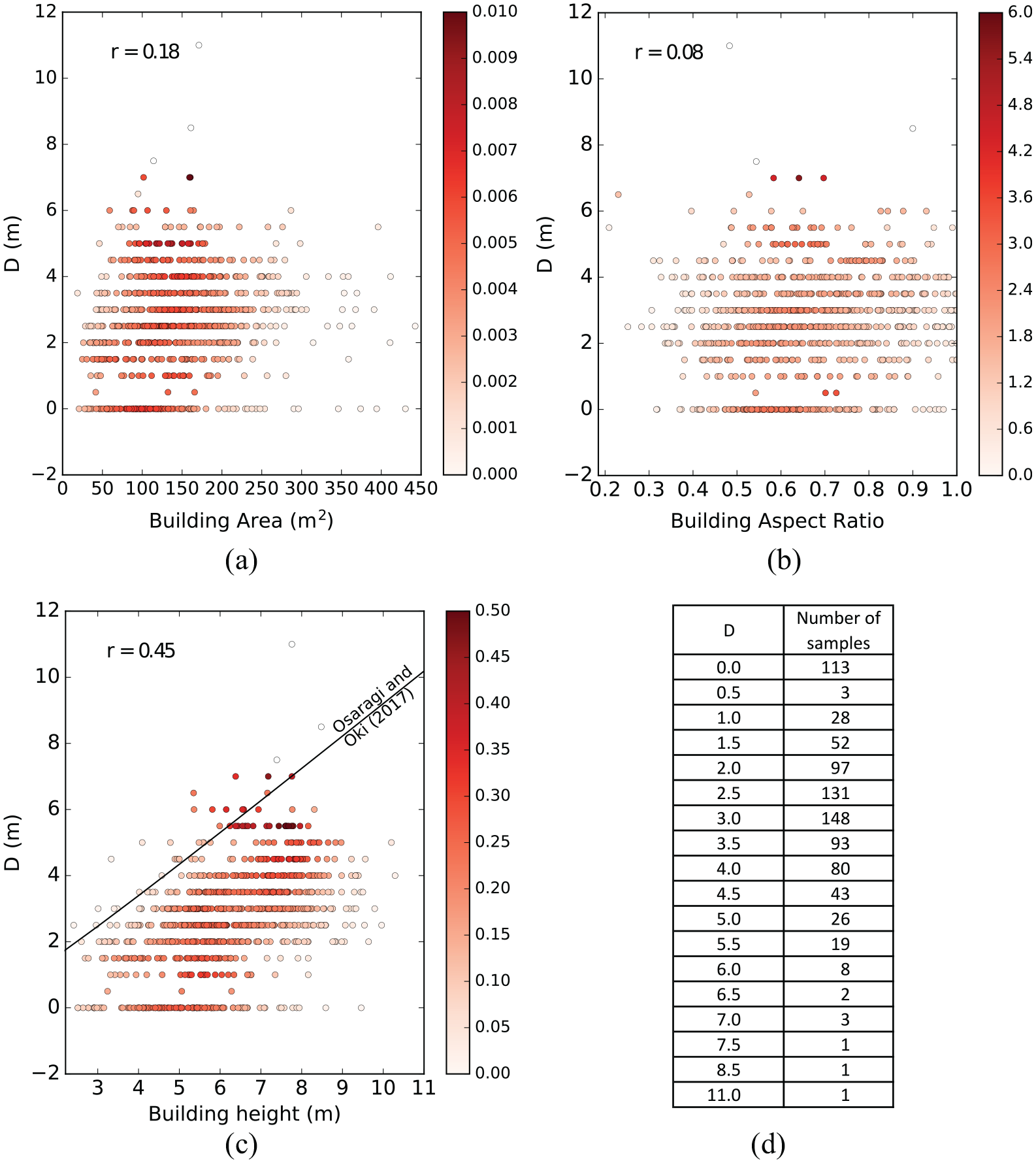
The Osaragi and Oki relationship between $H$ and w for $h' = 50 cm$ is plotted in Figure 9c as well. As expected, the estimations from Equation 1 are conservative compared with our measurements. However, both show a similar trend.

Figure 9.

Scatter plot of the debris extent, D, and some building geometrical features: (a) D versus building footprint area; (b) D versus building aspect ratio; (c) D versus building height, where the debris extent is a discrete variable that is multiples of 50 cm; (d) number of samples corresponding to each discrete value of D. The mark colors represent the kernel density estimated using Gaussian kernels of samples with the same value of D. The relationship height versus D assumed in the work of Osaragi and Oki (2017) is depicted in (c) as a solid black line. The correlation coefficient, r, is shown in the top left for each plot.

Probability functions for debris extent

As stated previously, the spatial distribution of the debris produced by a collapsed building is very complex, and thus it was not possible to propose a probabilistic model on the basis of the physical characteristics of the phenomena. Thus, the reader must be aware that this section aims to summarize the available data using smooth mathematical functions. With this purpose, a closer view of the samples is depicted in Figure 10. Here, histograms of several subsets constructed according to the building height are shown. The subsets were binned by intervals of 2 m. 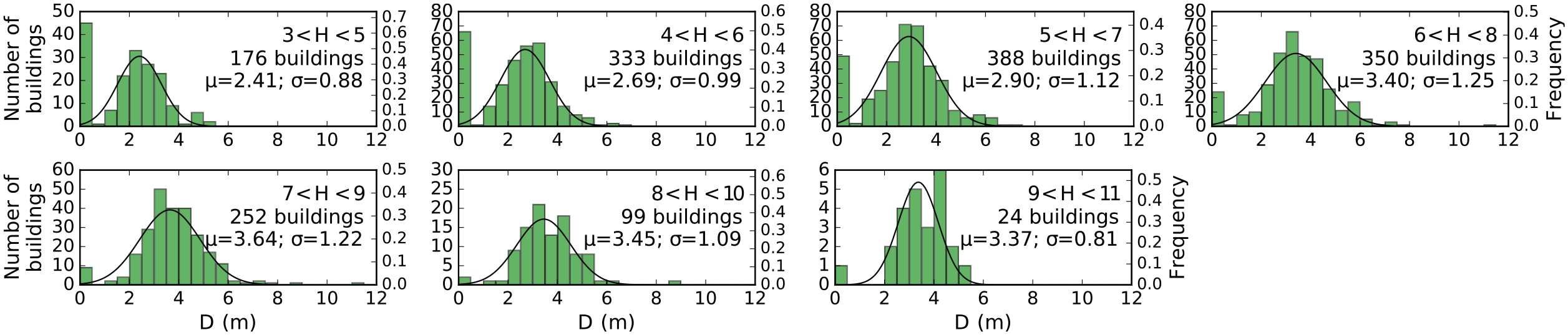Two main characteristics were observed: First, the fraction of buildings with $D = 0$ generates a spike in the distribution. Such fraction tends to decrease with the increasing building height. Second, samples with $D > 0$ are distributed in a rather smooth shape. The solid line shown in Figure 10 is a Gaussian function fitted from samples with $D > 0$ . Because of the spike observed at $D = 0$ , it was decided to break the distribution into two parts (McGuire, 2004): the fraction of collapsed buildings with no debris extent and the fraction of collapsed buildings that produced the debris extent.

Figure 10.

Distribution of D for buildings grouped by ranges of building height. The left-hand y-axis denotes the number of samples and the right-hand y-axis denotes the frequency. The solid line is a Gaussian function fitted from samples of $D > 0$ .

Regarding the samples with $D > 0$ , it is assumed that D is a random variable normally distributed with mean varying linearly with H and with uniform variance. The sample size is $n = 738$ . The mean value and the variance were obtained by the least squares method:

μ_{h} = β h + α = 0.31 h + 1.10,

(2)

σ = 1.11,

(3)

where $h$ denotes a particular realization of the random value H. The variance of the slope $β$ shown in Equation 2 is computed as follows:

σ_{B}^{2} = \frac{σ^{2}}{{ns}_{H}^{2}} = \frac{1.11 h^{2}}{738 \times 2.211} = 0.00075,

(4)

where $s_{H}^{2}$ is the variance of the building height. The value $σ_{B}$ is required to test whether there is a significant dependence of $μ_{h}$ on h. To this end, the null hypothesis is assumed. That is, the true slope in the linear relation is zero (i.e. $β = 0$ ). For this case, the accepted interval for the estimated slope at the 10% significance level is

\begin{matrix} - t_{0.05, n - 2} σ_{B} \leq B \leq t_{0.05, n - 2} σ_{B} \\ (- 1.647) (0.0274) \leq B \leq (1.674) (0.0274) \\ - 0.045 \leq B \leq 0.045, \end{matrix}

(5)

where $t_{0.05, n - 2}$ is the value at which the t cumulative distribution function, with $n - 2$ degrees of freedom, equals 0.95. Since our estimated slope $β = 0.31$ lies outside the interval $\pm 0.045$ , we reject the null hypothesis, that is, there is a significant dependence of $μ_{h}$ on h. Figure 11a shows the linear relation between $μ_{h}$ and h. The limits of $μ_{h} \pm σ_{h}$ and the 90% confidence of $μ_{h}$ are depicted as well. At this stage, the probability that $D = d$ adding the condition that $D > 0$ can be expressed as

P [D = d | D > 0 AND H = h AND collapse] = \frac{1}{\sqrt{2 π σ}} \exp [- \frac{{(d - μ_{h})}^{2}}{2 σ^{2}}] .

(6)

Figure 11.

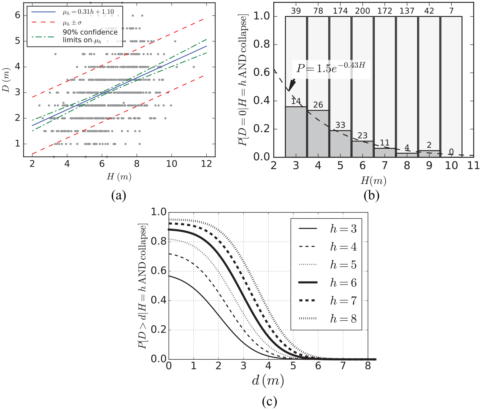
(a) Linear regression between building height $(H)$ and the debris extent $(D)$ for samples with $D > 0$ . The blue solid line denotes the linear relation between $μ_{h}$ and h obtained from the least squares method, the red dashed lines depict the limits of $μ_{h} \pm σ$ , and the green dashed-dot lines depict the 90% confidence limits of $μ_{h}$ . (b) Ratio of collapsed buildings with zero debris extent for different ranges of H. The number of samples with $D = 0$ and the total number of samples are reported for each bin. The solid line denotes an exponential function fitted from the observations. (c) Probability that a collapsed building of a given height h produces a debris extent greater than d.

Regarding the collapsed buildings with $D = 0$ , Figure 11b shows the fraction of samples with $D = 0$ within subsets binned by their height at intervals of 1 m. An exponential function is fitted to represent the observations. It is worth mentioning that the fraction of the bin $9.5 < h \leq 10.5$ was not used during the fitting because of the low number of samples in this bin. Then, the probability of $D = 0$ is expressed as follows:

P [D = 0 | H = h AND collapse] = 1.5 e^{- 0.43 h} .

(7)

And its complement represents the probability of $D > 0$ as follows:

P [D > 0 | H = h AND collapse] = 1 - 1.5 e^{- 0.43 h} .

(8)

The probability that $D = d$ is defined using Equations 2, 3, and 6 to 8 as follows:

P [D = d | H = h AND collapse] = {\begin{matrix} 1.5 e^{- 0.43 h}, d = 0 \\ (1 - 1.5 e^{- 0.43 h}) (\frac{1}{\sqrt{2 π σ}} \exp [- \frac{{(d - μ_{h})}^{2}}{2 σ^{2}}]), d > 0 \end{matrix} .

(9)

A useful parameter for the risk analysis of roads might be the probability that the debris extent will exceed certain value, $D > d$ :

P [D > d | H = h AND collapse] = \int_{d}^{\infty} P [D = x | H = h AND collapse] dx .

(10)

The differential term $dx$ on the rightmost side of Equation 10 should not be confused with the debris parameter d. Figure 11c shows the probability of exceeding d for different building heights. Notice that $P [D > d | H = h AND collapse]$ increases with the increasing building height h.

Applications

Probability of road blockage

To better clarify the usefulness of these probability functions in the context of seismic risk, the evaluation of a simple road was performed. Let us assume the existence of a road surrounded by only three wooden buildings of 7 m height and 8 m width (see Figure 12). For the sake of simplification, and to avoid the definition of damage levels on roads, only the probability that the road will be blocked was evaluated. A blockage of a road was assumed when the debris extended for more than a half of the road width. Thus, according to Figure 12, the probability that a building will produce debris with a length larger than 2.5 m needs to be calculated. Recall that Equation 10 was defined using the sample space of collapsed buildings, which is a subsample of all buildings. Therefore, the probability that a building will collapse is required.

Figure 12.

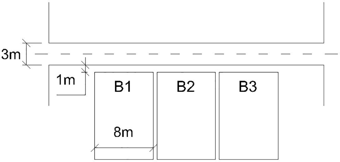
Case study of a road surrounded by three wooden buildings of 7 m height. The road has a width of 3 m and is at a distance of 1 m from the building facade. It is assumed that the buildings were constructed in between 1972 and 1981.

Fragility curves are used to estimate the probability of a building collapse (Porter et al., 2007). Generally, a fragility curve for a damage state dm is defined as the probability that an asset reaches or exceeds damage dm under a particular engineering demand parameter (EDP) value. Empirical fragility curves constructed for buildings in Japan have been proposed in previous studies (Horie et al., 2004; Yamazaki and Murao, 2000). Fragility functions are usually represented by a lognormal cumulative distribution function:

F_{dm} (edp) = Φ (\frac{\ln (edp) - λ}{β_{f}}),

(11)

where $Φ$ is the standard normal cumulative distribution function, $λ$ is the logarithmic median value, and $β_{f}$ is the logarithmic standard deviation. According to the buildings’ performance, a different set of fragility curves can be created for different construction materials and construction periods. For our example, the fragility curve for collapsed buildings proposed by Horie et al. (2004) was employed. Here, the peak ground velocity (PGV) is used as the EDP. Table 1 shows the values of $λ$ and $β_{f}$ for wooden buildings of different construction periods. Assuming an event that produced PGV = 170 cm/s in the case study and considering that the three wooden houses were built within the period of 1972–1981, the probability of collapse becomes

Table 1.

Parameters of fragility functions for wooden buildings (Horie et al., 2004)

	–1945	1946–1955	1956–1960	1961–1964	1965–1971	1972–1981	1982–1994
$λ$	4.69	4.83	4.93	5.03	5.24	5.62	6.52
$β_{f}$	0.39	0.37	0.41	0.45	0.54	0.54	0.81

F_{collapse} (PGV = 170) = 0.185 .

(12)

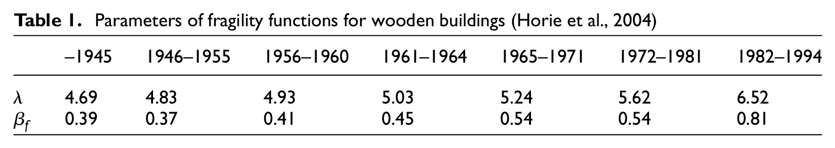
The probability that a collapsed building will produce debris with a length greater than 2.5 m is

P [D > 2.5 | H = 7 AND collapse] = 0.700 .

(13)

Finally, the probability that the building will block the road $(B)$ and its complement $(B^{c})$ are

B = (0.185) (0.700) = 0.129,

(14)

B^{c} = 1 - 0.127 = 0.871 .

(15)

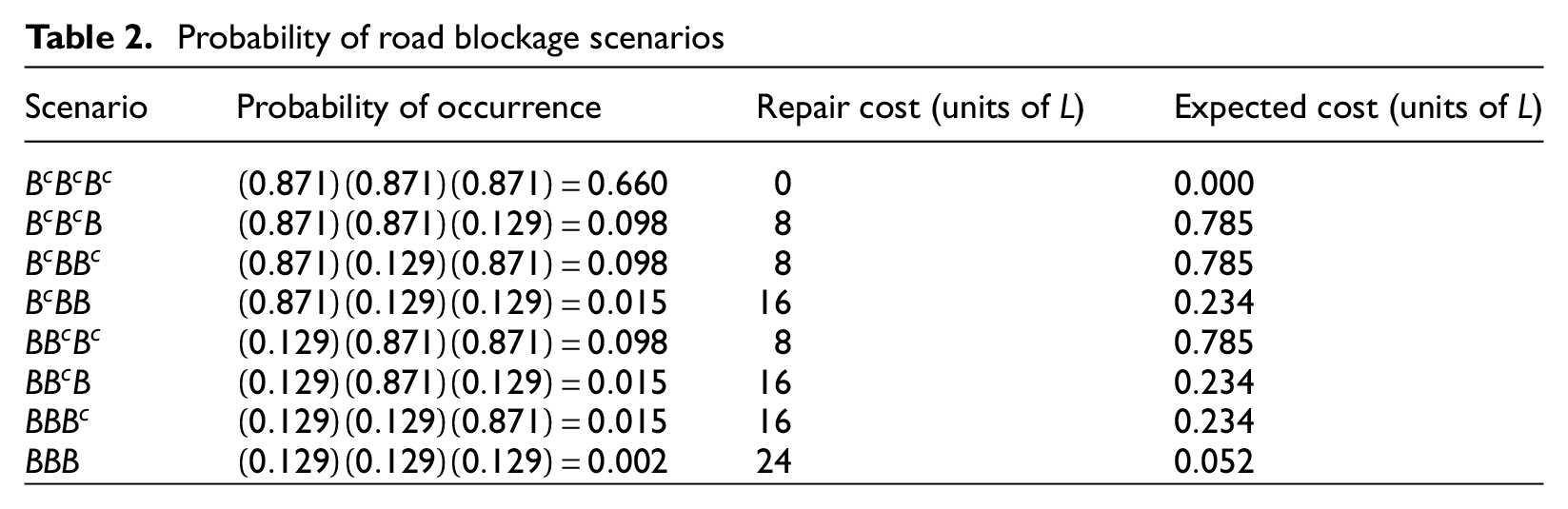
Let us now evaluate the different road blockage scenarios. The first column of Table 2 shows all the possible road blockage scenarios according to the outcomes of the three buildings. The second column shows the probability of occurrence for each scenario, and the variables are considered to be independent, that is, for example, the probability that the second building will block the road given that the first building blocked the road is still $B$ . From the second column, the probability that the road will be blocked is calculated as $(1 - B^{c} B^{c} B^{c}) = 0.340$ . The probability of blockage for N buildings with the same properties and spatial configurations as the buildings used in the example is shown in Figure 13a.

Table 2.

Probability of road blockage scenarios

Scenario	Probability of occurrence	Repair cost (units of L)	Expected cost (units of L)
$B^{c} B^{c} B^{c}$	$(0.871) (0.871) (0.871) = 0.660$	0	0.000
$B^{c} B^{c} B$	$(0.871) (0.871) (0.129) = 0.098$	8	0.785
$B^{c} B B^{c}$	$(0.871) (0.129) (0.871) = 0.098$	8	0.785
$B^{c} BB$	$(0.871) (0.129) (0.129) = 0.015$	16	0.234
$B B^{c} B^{c}$	$(0.129) (0.871) (0.871) = 0.098$	8	0.785
$B B^{c} B$	$(0.129) (0.871) (0.129) = 0.015$	16	0.234
$BB B^{c}$	$(0.129) (0.129) (0.871) = 0.015$	16	0.234
BBB	$(0.129) (0.129) (0.129) = 0.002$	24	0.052

Figure 13.

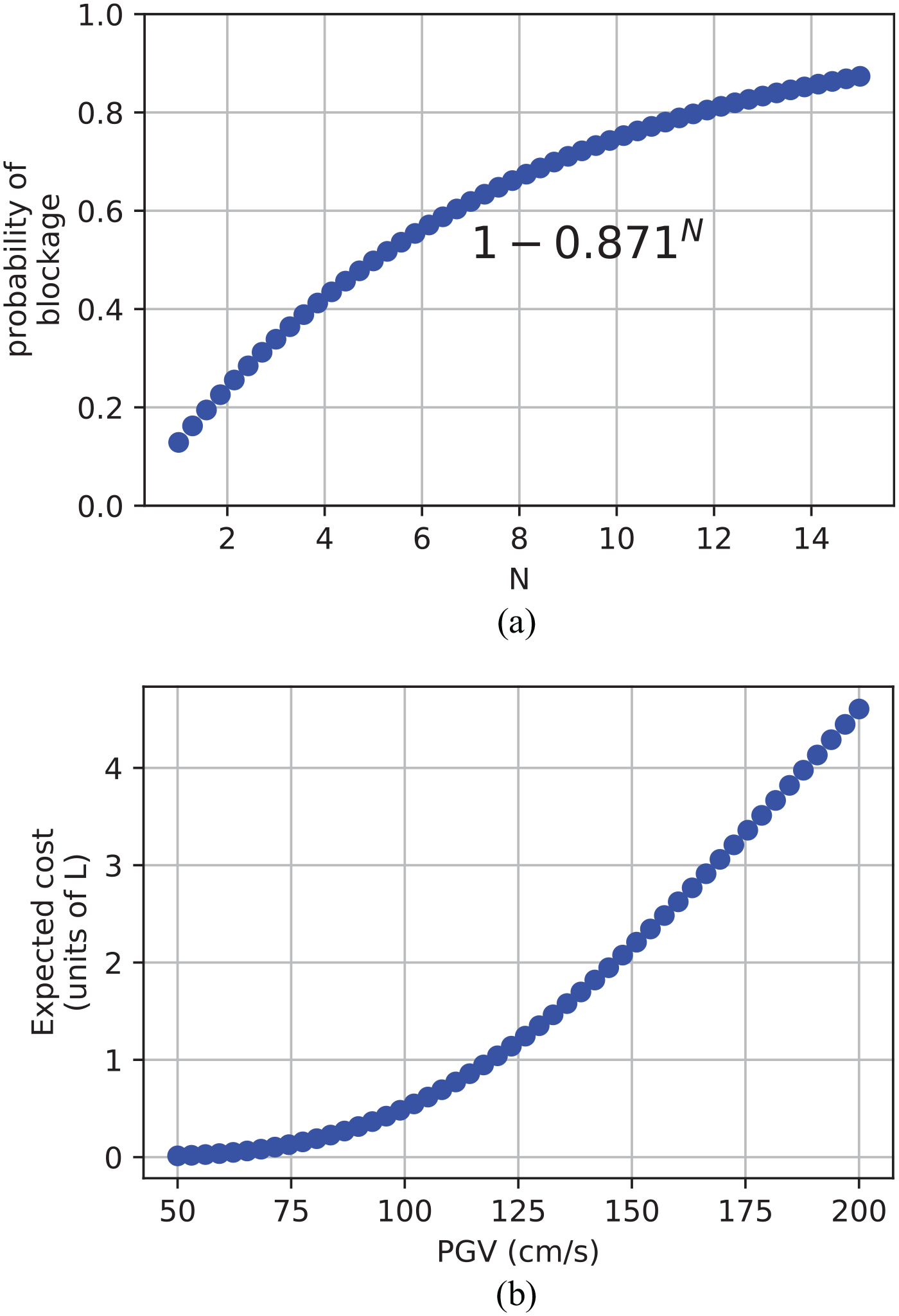
(a) Probability of road blockage for N buildings with characteristics similar to those shown in Figure 12 and placed on one side of a road; (b) expected cleaning cost of the road due to debris as a function of the PGV.

Consider a cost of L for removing a meter of blocked road due to debris. The cost required for each scenario is shown in the third column of Table 2. Here, the assumption that the debris width is equal to the building width was made. The expected cost can be calculated as the sum of the products between the probability of occurrence and their respective cost, both of which are shown in Table 2 as well. Thus, the expected cost for our simple road under a demand of 170 cm/s is 3.05L. Recall that the expected cost does not coincide with any actual cost that might occur. However, there are two good reasons for evaluating the risk in terms of loss (Erto et al., 2016): First, this approach provides a consistent way of treating the available information, and second it allows for a comparison with the risk of other consequences of the earthquake. Therefore, this method is very useful when risk management strategies are employed. In addition, it is possible to create profiles of an expected cost for a range of demand levels, such as that shown in Figure 13b.

Synthetic scenarios

In the previous section, the risk analysis of a road was performed by analyzing all of the possible scenarios of road blockage. However, this approach is applicable only for the simplest situations. The evaluation of isolated roads provides an estimation of its performance. However, risk analysis of the complete road network in terms of connectivity, capacity, and integrated loss estimation is more important. Obviously, because of the complexity of this task, evaluating all of the possible scenarios turns out to be inadequate. Under this situation, Monte Carlo simulations are perhaps the only way to conduct an analysis of road networks. Monte Carlo simulation has been used previously to simulate damage probability matrices, fragility curves, and vulnerability functions (Barbat et al., 1996). This approach is straightforward. The value of D is estimated from random numbers generated using a distribution calculated from Equations 2, 3, and 9. For that purpose, it is necessary to simulate the collapse/non-collapse behaviors of buildings first. Therefore, the spatial distribution of the demand and a database of buildings with information regarding the construction year and material of the structural system are required.

From hundreds or thousands of synthetic scenarios, it is possible to perform a probabilistic analysis of several issues, including the accessibility of specific targets, global expected cost, recognition of the most vulnerable areas, and relief distribution. Furthermore, these synthetic scenarios can be used to perform a more realistic simulation of evacuations of survivors and relief distribution (Das and Hanaoka, 2014; Mas et al., 2015; Nadi and Edrisi, 2017). As mentioned, the model for generating synthetic debris expansion must be implemented in a larger framework in which the damage states and the spatial distribution of the demand are included. This study is out of the scope of this article and will be addressed in a future study.

Discussion and conclusion

Using a pair of LiDAR datasets, aerial photos, and building footprint inventory data, in this article, the debris extent, D, produced by a wooden collapsed building was measured. The importance of D lies in that it is the main parameter used in methods proposed elsewhere to infer the post-earthquake functionality of road networks in urban areas. However, in previous studies, D has been estimated from simplified geometrical models, expert judgments, and/or observations occurred in earthquakes. This article represents the first time LiDAR data were used to quantify D, which provided an unprecedented opportunity to perform such measurements with a high accuracy. From the measurements, probability functions of D for wooden collapsed buildings in Japan were proposed. Thus, the proposed probability functions can contribute to estimate the interaction between the functionality of the road network and residential buildings.

After a selection process, a significant number of collapsed wooden buildings (851) were inspected, and their debris extents were carefully quantified, following the Mw 6.2 and Mw 7.0 events on, respectively, 14 and 16 April 2016, at the Kumamoto Prefecture, Japan. This study yielded the following findings: (1) A moderate correlation between the building height and the debris extent was observed. (2) The debris extent seems to have a Gaussian distribution. However, a fraction of the buildings did not produce debris. (3) The fraction of buildings without debris extent decreases when the building height increases. Based on these observations, probability functions for the debris extent were proposed. We believe that these results have some significance, and a simple case was evaluated in order to demonstrate its use. Furthermore, we identified that the proposed functions can contribute to constructing synthetic scenarios in which the debris extent can be modeled more realistically.

Additional details are necessary here regarding the selected collapsed buildings. The main goal was to select buildings for which the collapse patterns were not affected by any factors other than their own performance. Our main concern was the effects of the neighboring buildings. It would be desirable to isolate the study to buildings that are not closely located to other buildings. However, the number of buildings would have decreased significantly when performing the statistical evaluation. Therefore, it was decided to use all of the collapsed buildings for which the debris extent did not encounter any obstructions. We are not claiming that the effects of neighboring buildings were completely removed; however, decisions were made to reduce these effects to the minimum level. Moreover, we used the collapsed buildings extracted automatically by Moya et al. (2017b) from LiDAR datasets. From visual inspection, the non-collapsed buildings that were classified as collapsed were removed. However, the collapsed buildings classified as non-collapsed by Moya et al. (2017b) were not used in this study because of the effort it would require to visually verify these buildings among the thousands of non-collapsed buildings. We believe that there were only a small number of undetected collapsed buildings, and thus these buildings would not affect the statistical results.

It is highly probable that information of building failure mode would be strongly correlated with the debris extent. Unfortunately, from the LiDAR data, the characterization of building failure mode following current standards such as the EMS-98 was not viable. However, it should be noted that if the debris extent as a function of building failure mode would be available, its application for urban road network functionality assessment would require the probability of collapse under a specific failure mode, which is not often available. Fragility curves for collapsed buildings without considering the failure mode are more often available. It might be possible to correlate the building date of construction with the debris extent, but such information was not available as well. Material type should also be correlated with the debris extent, and therefore the probabilistic model proposed in this study applies only to wooden buildings.

Regarding the evaluation of a simple road, the conservative assumption that the debris direction was toward the road was made. In reality, this is not strictly necessary. However, debris tends to move toward the free sides of a building, and the buildings next to the road generally have two or three sides obstructed by neighboring buildings. The probability of blockage and the expected cost might be lower than our estimation if the debris directions were considered. Recall that this conservative assumption has also been made by the studies mentioned in the introduction. Another simple parameter used was the unit cost to remove the debris from the road, L. It may be necessary to consider additional information, such as the expected weight of the debris and the transportation to a disposal site. However, this information varies according to the strategy of the decision makers. For instance, it was observed that within the early response the priority was to allow access and thus the debris was placed beside the roads, as can be observed in Figure 4g and h. Furthermore, if the reader is interested in reproducing the exercise with a more realistic case, it is important to note that additional steps are necessary for cases in which buildings are located along both sides of a road. In this case, the probability that a building will block the road is no longer independent. For instance, assume the case in which a pair of buildings is located on both sides of a building and in which one is in front of the other. With $D_{1}$ and $D_{2}$ representing the debris produced by the two buildings, the probability that the road will be blocked at the location of these buildings is the probability that $D_{1} + D_{2}$ will exceed some percentage of the road width. There is a body of literature that deals with the sum of two random variables (for instance, Benjamin and Cornell, 1970).

This article focuses on road blockage due to building debris. However, accessibility to road networks after disasters depends on several other factors, such as damage to bridges (Yamazaki et al., 2000), ground failure, and landslides. Argyroudis et al. (2015) present a summary of all the possible sources of road blockages. Therefore, our outputs must be used within an integrated framework in which all of the possible types of damage that might induce road network blockage are included.

Footnotes

Acknowledgements

The authors acknowledge the Asia Air Survey Co., Ltd, Japan for providing the LiDAR data. In addition, the authors would like to thank the anonymous reviewers for their insightful comments and constructive suggestions.

Authors' Note

Fumio Yamazaki is currently affiliated with National Research Institute for Earth Science and Disaster Resilience, 3-1 Tennodai, Tsukuba, Ibaraki, Japan

Declaration of conflicting interests

The author(s) declared no potential conflicts of interest with respect to the research, authorship, and/or publication of this article.

Funding

The author(s) disclosed receipt of the following financial support for the research, authorship, and/or publication of this article: This research was supported by the Japan Science and Technology Agency (JST) through the SICORP project “Increasing Urban Resilience to Large Scale Disaster: The Development of a Dynamic Integrated Model for Disaster Management and Socio-Economic Analysis (DIM2SEA)” (no. J150002645) and the CREST project no. (JP-MJCR1411), and the Japan Society for the Promotion of Science (JSPS) Kakenhi (17H06108). The authors thank the Core Research Cluster of Disaster Science at Tohoku University (a designated national university) for their support.

References

Argyroudis

Selva

Gehl

, et al. (2015) Systemic seismic risk assessment of road networks considering interactions with the built environment. Computer-Aided Civil and Infrastructure Engineering 30: 524–540.

Asia Air Survey Co., Ltd. (2016) The 2016 Kumamoto earthquake. Available at: http://www.ajiko.co.jp/article/detail/ID5725UVGCD/ (accessed 8 September 2017).

Axel

van Aardt

JAN

Aros-Vera

, et al. (2016) Remote sensing-based detection and quantification of roadway debris following natural disasters. Proceedings of SPIE 9832: 98320C.

Barbat

Moya

Canas

(1996) Damage scenarios simulation for seismic risk assessment in urban zones. Earthquake Spectra 12: 371–394.

Benjamin

Cornell

(1970) Probability, Statistics and Decisions for Civil Engineers. New York: McGraw Hill.

Cabinet Office of Japan (2017) Summary of damage situation in the Kumamoto earthquake sequence. Available at: http://www.bousai.go.jp/updates/h280414jishin/index.html (accessed 7 August 2017).

Das

Hanaoka

(2014) An agent-based model for resource allocation during relief distribution. Journal of Humanitarian Logistics and Supply Chain Management 4: 265–285.

Dolce

(2012) The Italian national seismic prevention program. In: Proceedings of the 15th world conference on earthquake engineering (Invited Lecture), Lisbon, 24–28 September.

Erto

Giorgio

Iervolino

(2016) About knowledge and responsibility in probabilistic seismic risk management. Seismological Research Letters 87: 1161–1166.

10.

Eshghi

Ahari

(2005) Performance of transportation systems in the 2003 Bam, Iran, earthquake. Earthquake Spectra 21: 455–468.

11.

Gordon

Richardson

Davis

(1998) Transport-related impacts of the Northridge earthquake. Journal of Transportation and Statistics 1: 21–36.

12.

Goretti

Sarli

(2006) Road network and damaged buildings in urban areas: Short and long-term interaction. Bulletin of Earthquake Engineering 4: 159–175.

13.

Horie

Hayashi

Okimura

, et al. (2004) Development of seismic risk assessment method reflecting building damage levels—Fragility functions for complete collapse of wooden buildings. In: Proceedings of the 13th world conference on earthquake engineering (No. 2240), Vancouver, BC, Canada, 1–6 August.

14.

Japan Meteorological Agency (2017) The number of aftershocks of recent inland earthquakes in Japan. Available at: http://www.data.jma.go.jp/svd/eqev/data/2016_04_14_kumamoto/kaidan.pdf. (accessed 7 August 2017).

15.

Liu

Yamazaki

(2017) Extraction of collapsed buildings in the 2016 Kumamoto earthquake using multi-temporal PALSAR-2 data. Journal of Disaster Research 12: 241–250.

16.

McGuire

(2004) Seismic Hazard and Risk Analysis (Engineering Monographs on Miscellaneous Earthquake Engineering Topics). Oakland, CA: Earthquake Engineering Research Institute, pp. 145–153.

17.

Maruyama

Itagaki

(2017) Development of tsunami fragility functions for ground-level roads. Journal of Disaster Research 12: 131–136.

18.

Mas

Koshimura

Imamura

, et al. (2015) Recent advances in agent-based tsunami evacuation simulations: Case studies in Indonesia, Thailand, Japan and Peru. Pure and Applied Geophysics 172: 3409–3424.

19.

Moya

Mas

Adriano

, et al. (2017a) Building damage mapping using change detection of ALOS-2 PALSAR-2 SAR images and strong motion data. In: International symposium on remote sensing (D-22), Nagoya, Japan, 17–19 May.

20.

Moya

Yamazaki

Liu

, et al. (2017b) Calculation of coseismic displacement from Lidar data in the 2016 Kumamoto, Japan, earthquake. Natural Hazards and Earth System Sciences 17: 143–156.

21.

Moya

Yamazaki

Liu

, et al. (2017c) Detection of collapsed buildings due to the 2016 Kumamoto, Japan, earthquake from Lidar data. Natural Hazards and Earth System Sciences Discussions 18: 65–78.

22.

Nadi

Edrisi

(2017) Adaptive multi-agent relief assessment and emergency response. International Journal of Disaster Risk Reduction 24: 12–23.

23.

Okada

Takai

(2000) Classification of structural types and damage patterns of buildings for earthquake field investigation. In: Proceedings of the 12th world conference on earthquake engineering (No. 0705), Auckland, New Zealand, 30 January–4 February.

24.

Osaragi

Oki

(2017) Wide-area evacuation simulation incorporating rescue and firefighting by local residents. Journal of Disaster Research 12: 296–310.

25.

Porter

Kennedy

Bachman

(2007) Creating fragility functions for performance-based earthquake engineering. Earthquake Spectra 23: 471–489.

26.

Sato

Kanagawa

Spinks

(1996) Survey on commute and work pattern changes after the Great Hanshin earthquake. International Flexwork Forum 5, http://www.telework-gakkai.jp/archive/IFF/english/issues/V5n20/7.html

27.

Scawthorn

Rathje

(2006) The 2004 Niigata Ken Chuetsu, Japan, earthquake. Earthquake Spectra 22: 1–8.

28.

Scott

(1992) Multivariate Density Estimation: Theory, Practice, and Visualization. Hoboken, NJ: Wiley.

29.

Texas Department of Transportation (2017) Drive TEXAS TxDOT highway conditions. Available at: https://drivetexas.org/#/8/30.113/-96.594?future=false (accessed 8 September 2017).

30.

UNEP/OCHA (2011) Disaster Waste Management Guidelines (Technical Report). Geneva: Joint UNEP/OCHA Environment Unit.

31.

Yamada

Ohmura

Goto

(2017) Wooden building damage analysis in Mashiki Town for the 2016 Kumamoto earthquakes on April 14 and 16. Earthquake Spectra 33: 1555–1572.

32.

Yamazaki

Liu

(2016) Remote sensing technologies for post-earthquake damage assessment: A case study on the 2016 Kumamoto earthquake. In: Proceedings of the 6th Asia conference on earthquake engineering (KN4), Cebu City, Philippines, 22–24 September.

33.

Yamazaki

Murao

(2000) Vulnerability functions for Japanese buildings based on damage data from the 1995 Kobe earthquake. In: Implications of recent earthquakes on seismic risk, London, 6–7 April, vol. 2, pp. 91–102. London, UK: Imperial College Press.

34.

Yamazaki

Motomura

Hamada

(2000) Damage assessment of expressway networks in Japan based on seismic monitoring. In: Proceedings of the 12th world conference on earthquake engineering (No. 0551), Auckland, New Zealand, 30 January–4 February.

35.

Zanini

Faleschini

Zampieri

, et al. (2017) Post-quake urban road network functionality assessment for seismic emergency management in historical centres. Structure and Infrastructure Engineering 13: 1117–1129.