Next-generation liquefaction database

Abstract

The Next-Generation Liquefaction database is a resource for the geotechnical hazard community. It is publicly available online under the following digital object identifier (DOI): 10.21222/C2J040. The database organizes objective liquefaction data into tables and fields (columns of information), with the relationships among the tables and fields described by a schema. The data are organized into tables pertaining to (1) sites, including geotechnical and geophysical site investigation data, surface geology information, and laboratory test data; (2) earthquake events, including source and ground motion information; and (3) observations of sites following events. The schema was vetted through community outreach efforts involving multiple workshops and meetings. Users can view the data, download existing data, and upload new data through a geographic information system (GIS)-based graphical user interface. Information uploaded to the database is reviewed by a database working group to verify consistency between uploaded data and source documents. The database is replicated in DesignSafe where users can interact with the data using Python scripts in Jupyter notebooks, view point cloud data using Potree, and interact with geospatial data using QGIS.

Keywords

Liquefaction database Jupyter geotechnical observation site investigation

Introduction

For analysis of liquefaction-related hazard at the scale of individual projects, semi-empirical procedures are used to evaluate liquefaction susceptibility, triggering, and effects. These procedures combine empirical observations with various aspects of theory. Measurements of penetration resistance (standard penetration test, SPT, blow count or cone penetration test, CPT, resistance) or shear wave velocity (V_S ) are generally utilized to assess soil resistance to liquefaction. Surface ground motion parameters are combined with wave propagation theory to estimate stress demands at a particular depth, and this demand is compared with resistance to obtain a factor of safety or the probability of liquefaction given a certain event. Examples of such procedures include Seed et al. (1983), Cetin et al. (2004, 2018), and Idriss and Boulanger (2012) (SPT procedures); Robertson and Wride (1998), Moss et al. (2006), and Boulanger and Idriss (2016) (CPT procedures); and Andrus and Stokoe (2000) and Kayen et al. (2013) (V_S procedures). For applications at regional scales, qualitative geology-based criteria are used to estimate relative levels of liquefaction resistance (Lewis et al., 1999; Obermeier et al., 1990; Youd and Hoose, 1978; Youd and Perkins, 1978). In a similar manner, liquefaction resistance at the regional scale can be modeled using geospatial variables (Zhu et al., 2015, 2017).

A shared attribute of both approaches is their reliance on empirical data from sites and regions that have or have not experienced surface manifestations of liquefaction following earthquakes. For this reason, procedures for evaluating liquefaction rely strongly on empirical data. This reliance on data is not unique to liquefaction research. An analogous data-driven model development approach has been adopted by the various Next-Generation Attenuation (NGA) projects (e.g. NGA-West2, Bozorgnia et al., 2014, for shallow crustal earthquakes in active tectonic regions; NGA-East, Goulet et al., 2018, for stable continental regions; and NGA-Subduction, Bozorgnia et al., 2020, for subduction events). The Pacific Earthquake Engineering Research Center established the Next Generation Liquefaction (NGL) project to facilitate a similar process for modeling liquefaction triggering and consequences, a key component of which is the establishment of a community database of liquefaction-related case histories. In this paper, we describe that database.

Variations over time of the cumulative numbers of case histories in the SPT, CPT, and V_S liquefaction databases are presented in Figure 1 along with the cumulative numbers of ground motion records in the NGA-West2 and NGA-Subduction projects. The number of ground motion records in the NGA projects has grown exponentially with time, as indicated by the essentially linear slope in semi-log space in Figure 1. The liquefaction databases, by contrast, show essentially exponential growth from about 1960 to 1995, but the growth has slowed recently, with very few new case histories introduced into these databases since 1995. This trend is not due to a lack of available data. For example, the Canterbury Earthquake Sequence in 2010 and 2011 produced tens of thousands of CPTs with observations of ground performance during multiple earthquakes (e.g. Maurer et al., 2014a; van Ballegooy et al., 2014; Cubrinovski et al. 2019). Furthermore, post-1995 earthquakes that have produced potential liquefaction case history information include: 1999 Kocaeli, Turkey, 1999 Chi-Chi, Taiwan, 1999 Duzce, Turkey, 2001 Bhuj, India, 2001 Nisqually, Washington, 2001 Peru, 2002 Denali, Alaska, 2004 Niigata Chuetsu-Oki, Japan, 2007 Niigata Ken Chuetsu-Oki, Japan, 2007 Pisco, Peru, 2008 Iwate, Japan, 2009 L’Aquila, Italy, 2010 Maule, Chile, 2010 El Mayor Cucapah, Mexico, 2011 Tohoku-Oki, Japan, 2012 Emilia, Italy, 2015 Nepal, 2016 Kaikoura, New Zealand, 2017 Puebla, Mexico, 2018 Hokkaido Eastern Iburi, Japan, 2018 Anchorage, Alaska, and 2019 Ridgecrest, California.

Figure 1.

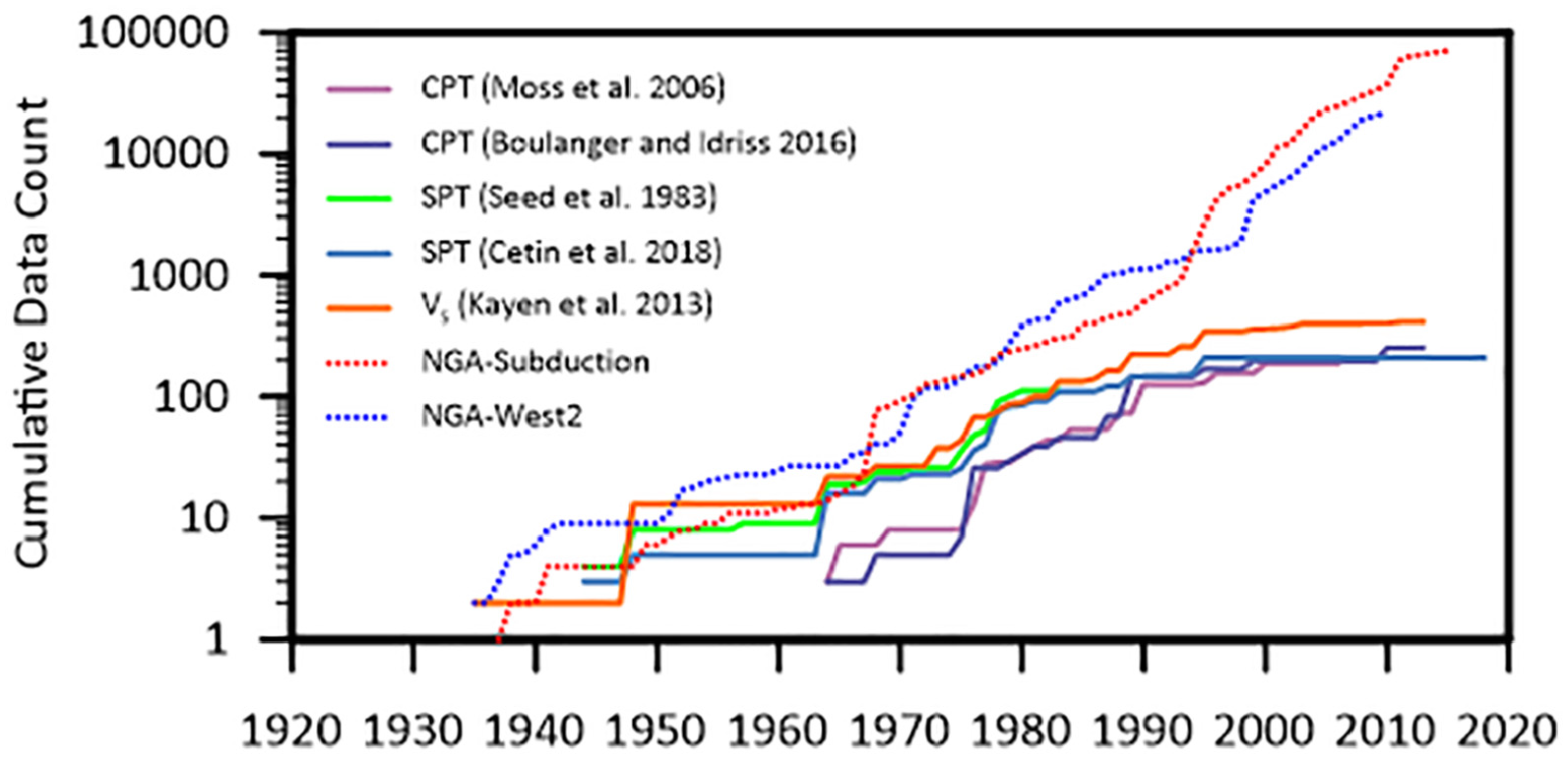
Cumulative number of liquefaction case histories utilized in various triggering models and ground motion records in the NGA-West2 and NGA-Subduction projects.

We believe that liquefaction case history databases have lagged behind the exponential growth exhibited by the ground motion databases because the NGA projects involved a broad community effort surrounding database development, whereas development of liquefaction datasets has largely been undertaken by small research groups (i.e. Seed et al., 1983 and Çetin et al., 2004, 2018 for SPT data, Moss et al., 2006 for CPT data, Kayen et al., 2013 for V_S data, and Zhu et al. 2015 for geospatial data) without a broader organizational framework. A larger community effort is needed to optimize the potential to learn from recent events and grow the liquefaction database both in size and quality. The need for a publicly available liquefaction database was the first recommendation of the committee commissioned by the National Academies of Sciences, Engineering, and Medicine to address the state of the art and practice in assessment of earthquake-induced liquefaction and its consequences (National Academies of Sciences, Engineering, and Medicine, 2016):

Recommendation 1. Establish curated, publicly accessible databases of relevant liquefaction triggering and consequence case history data. Include case histories in which soils interact with built structures. Document the case histories with relevant field, laboratory, and physical model data. Develop the databases with strict protocols and include indicators of data quality.

The NGL project was designed in part to address this clear need. NGL is a multi-year community-based effort consisting of three components: (1) a transparent, open-source liquefaction database; (2) supporting studies for effects that should be captured in models but that cannot be constrained by case history data; and (3) model development (Stewart et al., 2016).

This article presents the structure of the NGL relational database and the graphical user interface (GUI) developed to upload, view, and download data. We also discuss the review process implemented to ensure that uploaded data are consistent with source documents. The GUI allows users to interact with the data in a limited manner, but model developers will need to work with the data in ways that are not implemented in the GUI. For this reason, the database is periodically replicated in DesignSafe, a cyberinfrastructure for the natural hazards community (Rathje et al., 2017a). This allows users to formulate their own queries, perform high-level data analysis, integrate geospatial datasets, and draw conclusions. We discuss several publicly available tools in DesignSafe and provide example queries to extract desired data and show examples of geospatial data integration.

NGL database structure

The NGL database is a relational database, meaning that it has a well-defined data structure and can be queried using structured query language (SQL). The term “database” is often informally applied to file repositories lacking a formal organizational structure. In contrast, a relational database is organized into a schema that describes the tables, fields, and relationships among tables. In this context, a table is a collection of information containing a series of fields (or columns). Database fields are related using keys. Every entry in the database is assigned a primary key that uniquely identifies the field. In some cases, a field from one table might appear in another table to relate the two tables. In this case, the primary key from the host table appears as a foreign key in the other table to map the relationship.

The NGL database schema was developed over a number of years by a database working group and vetted by an interested community of geotechnical earthquake engineers through a series of public workshops. Draft versions of the database were presented during workshops at the University of California, Berkeley, in July 2017 and at the University of California, Los Angeles in September 2018. The database schema presented here is the product of that process. While the database structure is essentially complete, population of the database is ongoing and is anticipated to continue indefinitely as additional data become available.

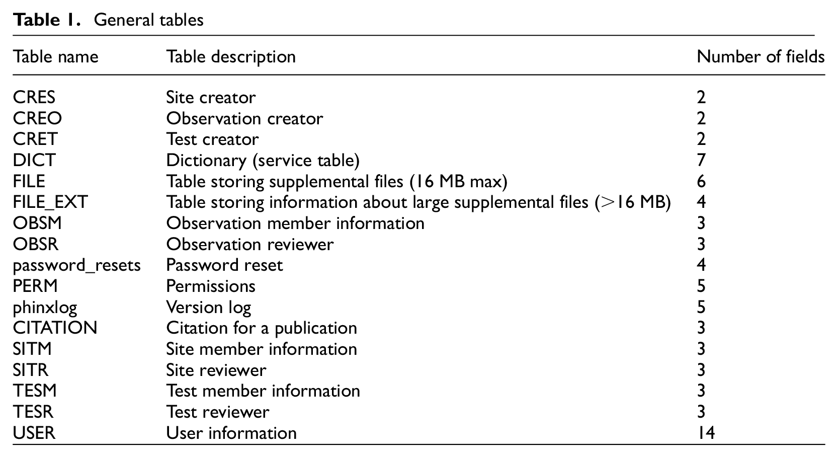
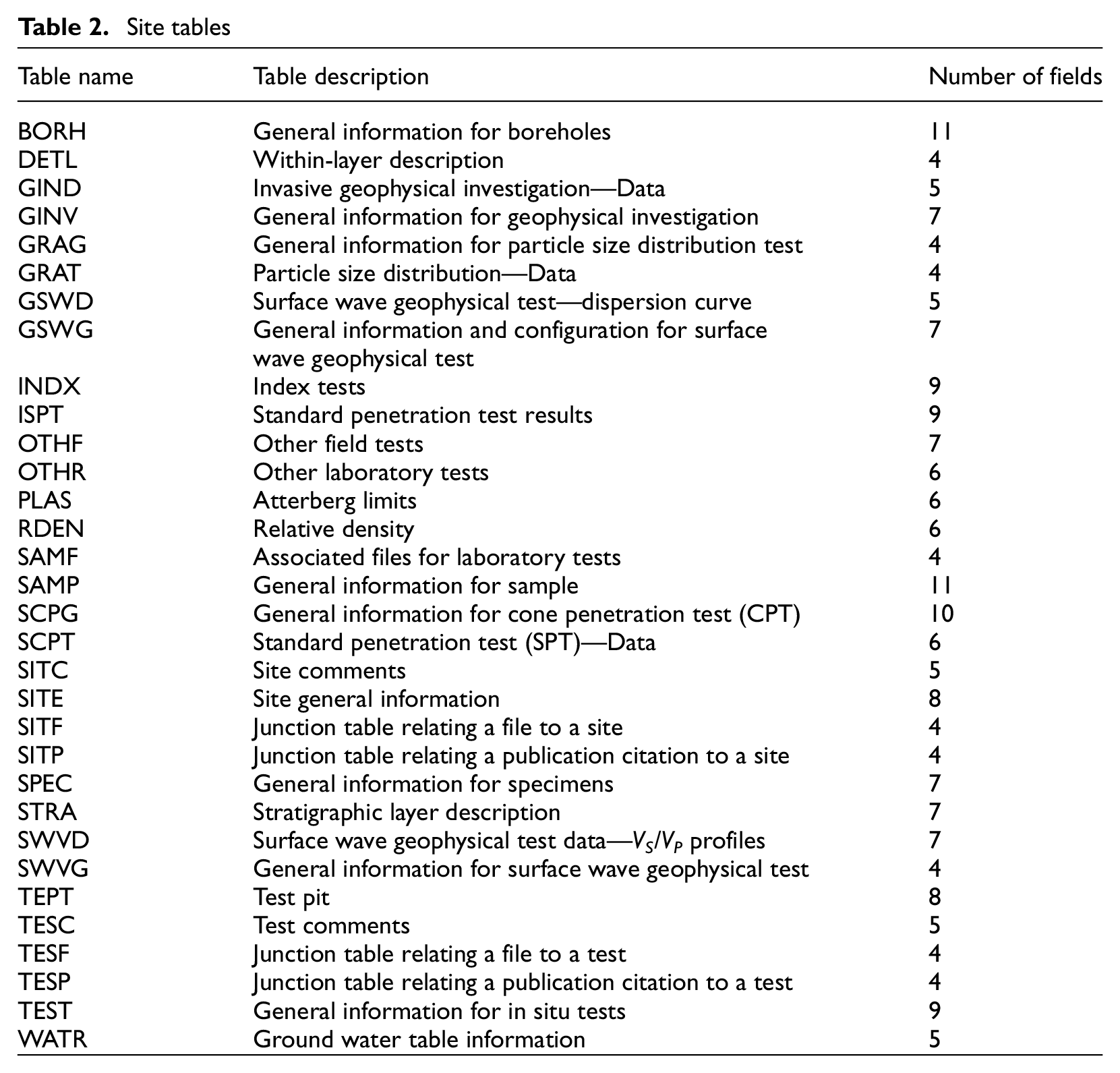
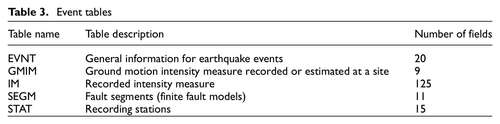
The NGL database consists of 60 tables that can be broadly categorized as general, site, event, and observation (Tables 1 to 4, respectively). The general tables contain fields about the users, reviewers, project team members, and miscellaneous tables related to permissions, password reset requests, and version logs. The general tables also contain fields for file uploads and citations of published datasets or other publications. The site tables contain geotechnical/geological information such as CPT data, SPT data, soil layer descriptions (as in borehole logs), geophysical measurements, laboratory tests, and groundwater table depth. Geospatial data, such as geology maps and digital elevation models, may also be included with or linked to a specific site. The event tables contain information about the earthquake source, recording stations, and ground motion intensity measures from recordings (if available). The observation tables contain results of post-earthquake reconnaissance at the site, which may include photographs, maps, measured ground deformations, commentary on the presence of liquefaction surface manifestation or lack thereof, and links to large datasets such as light detection and ranging (LIDAR), structure from motion (SfM), or geospatial raster files.

Table 1.

General tables

Table name	Table description	Number of fields
CRES	Site creator	2
CREO	Observation creator	2
CRET	Test creator	2
DICT	Dictionary (service table)	7
FILE	Table storing supplemental files (16 MB max)	6
FILE_EXT	Table storing information about large supplemental files (>16 MB)	4
OBSM	Observation member information	3
OBSR	Observation reviewer	3
password_resets	Password reset	4
PERM	Permissions	5
phinxlog	Version log	5
CITATION	Citation for a publication	3
SITM	Site member information	3
SITR	Site reviewer	3
TESM	Test member information	3
TESR	Test reviewer	3
USER	User information	14

Table 2.

Site tables

Table name	Table description	Number of fields
BORH	General information for boreholes	11
DETL	Within-layer description	4
GIND	Invasive geophysical investigation—Data	5
GINV	General information for geophysical investigation	7
GRAG	General information for particle size distribution test	4
GRAT	Particle size distribution—Data	4
GSWD	Surface wave geophysical test—dispersion curve	5
GSWG	General information and configuration for surface wave geophysical test	7
INDX	Index tests	9
ISPT	Standard penetration test results	9
OTHF	Other field tests	7
OTHR	Other laboratory tests	6
PLAS	Atterberg limits	6
RDEN	Relative density	6
SAMF	Associated files for laboratory tests	4
SAMP	General information for sample	11
SCPG	General information for cone penetration test (CPT)	10
SCPT	Standard penetration test (SPT)—Data	6
SITC	Site comments	5
SITE	Site general information	8
SITF	Junction table relating a file to a site	4
SITP	Junction table relating a publication citation to a site	4
SPEC	General information for specimens	7
STRA	Stratigraphic layer description	7
SWVD	Surface wave geophysical test data—V_S /V_P profiles	7
SWVG	General information for surface wave geophysical test	4
TEPT	Test pit	8
TESC	Test comments	5
TESF	Junction table relating a file to a test	4
TESP	Junction table relating a publication citation to a test	4
TEST	General information for in situ tests	9
WATR	Ground water table information	5

Table 3.

Event tables

Table name	Table description	Number of fields
EVNT	General information for earthquake events	20
GMIM	Ground motion intensity measure recorded or estimated at a site	9
IM	Recorded intensity measure	125
SEGM	Fault segments (finite fault models)	11
STAT	Recording stations	15

Table 4.

Observation tables

Table name	Table description	Number of fields
FLDD	Displacement vectors	8
FLDF	Junction table relating a file to an observation	6
FLDP	Junction table relating a publication citation to an observation	4
FLDM	Liquefaction manifestation	11
FLDO	General information for field observation	6
OBSC	Observation comment	5

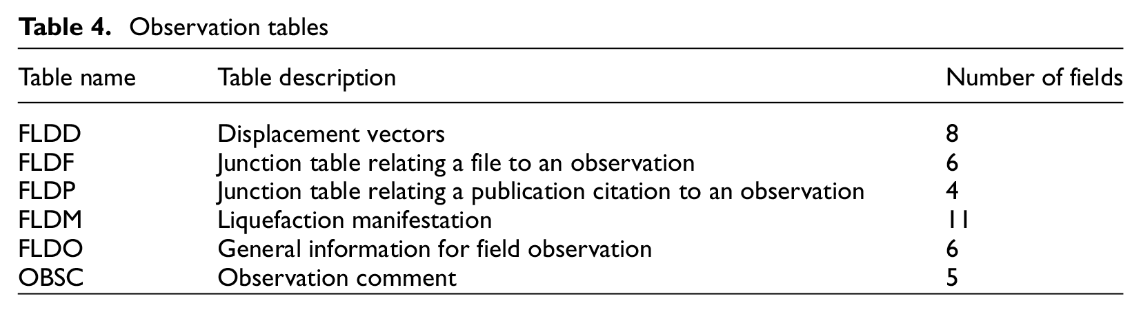
A total of 494 different fields are contained within the tables defined by Tables 1 through 4. A dictionary describing each individual field in these tables is provided in an interactive webpage: http://nextgenerationliquefaction.org/schema/index.html. The current schema at that web page is updated from an earlier version presented by Brandenberg et al. (2018), and any future changes will also be reflected in the online schema. Here, we describe several example tables to illustrate key aspects of database functionality.

Figure 2 shows example site investigation tables and fields, with arrows indicating the primary key/foreign key relationships between tables. A site consists of a primary key (SITE_ID), site name (SITE_NAME), latitude (SITE_LAT), longitude (SITE_LON), description of surface geology (SITE_GEOL), a remark about the site (SITE_REM), a Boolean field indicating whether the site has been submitted for review (SITE_STAT), and a Boolean field indicating whether the site has been reviewed (SITE_REVW). Minimum data requirements for the SITE table are SITE_NAME, SITE_LAT, and SITE_LON.

Figure 2.

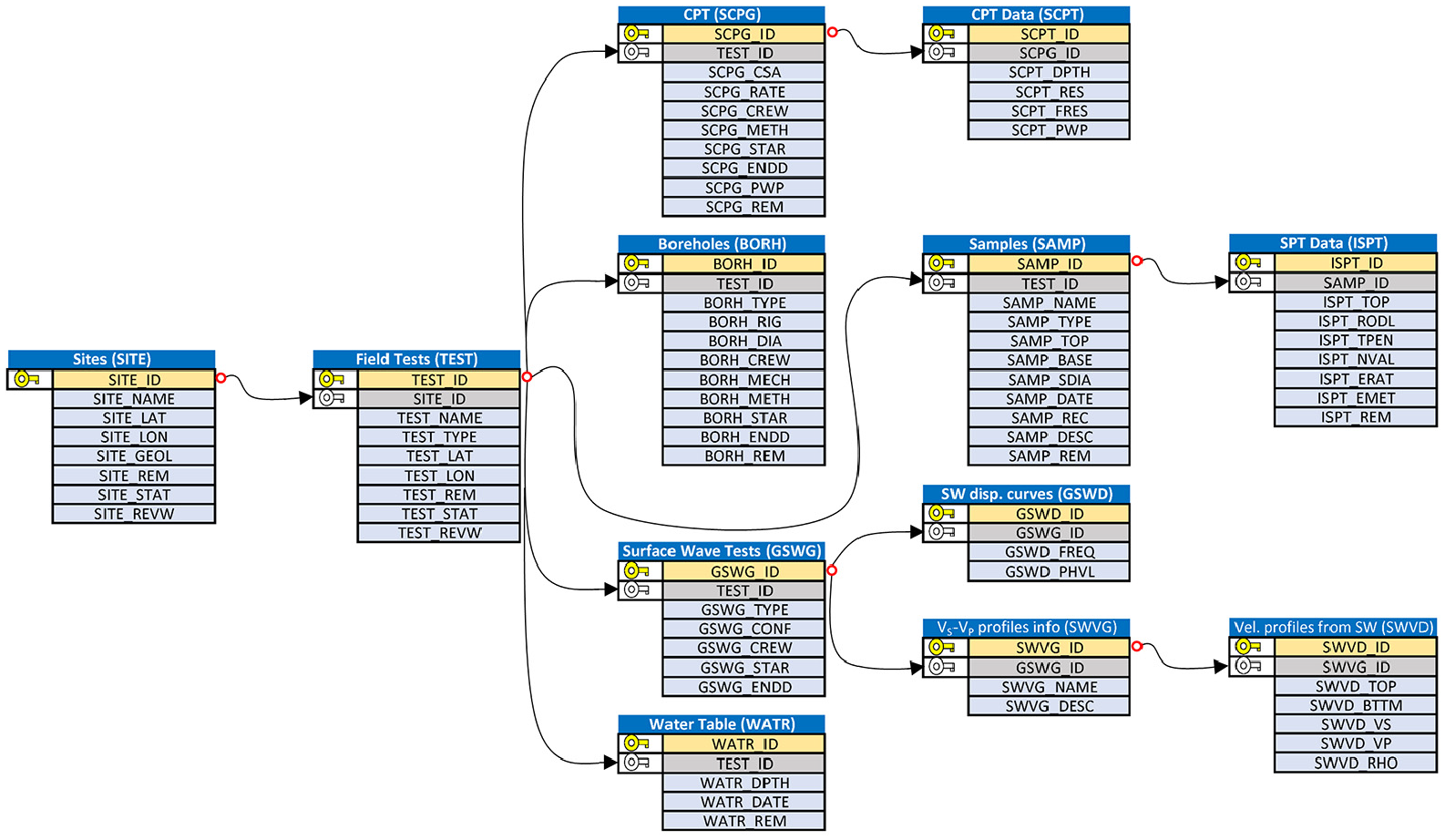
Subset of NGL relational database schema illustrating tables containing site investigation data.

Because the NGL database scheme uses the word “site,” an operational definition is required. A site is a high-level entity into which a team of NGL users organize their data. A site generally represents a contiguous geographical area that has been investigated by the team and for which observations of liquefaction effects have been made for an event or sequence of events. Latitude and longitude fields are required for each site so that the site can be located on the map within the GUI, but that does not mean that a site should be interpreted as a single location in space. Geotechnical conditions and observations of liquefaction effects may vary spatially within a site. Users must exercise judgment in assigning a specific geographical area to a site and are encouraged to provide a remark explaining their rationale for organizing the information with a site.

Once a site has been established, a test or set of tests used to evaluate site conditions may be defined for that site. Note that the TEST table has a SITE_ID field, which is a foreign key that links the TEST table with a particular SITE. In the TEST table TEST_NAME, TEST_TYPE, TEST_LAT, and TEST_LON are required fields. In this manner, multiple tests may be specified for a specific site without the need for repeating information from the site table. The types of tests illustrated in Figure 2 include CPT (SCPG), borehole (BORH), surface wave geophysical test (GSWG), groundwater table measurement (WATR), and sample (SAMP). As shown in Figure 2, an individual test has a location, which does not necessarily align with that of the SITE. Although not shown in Figure 2, additional test types, including stratigraphy (STRA), detailed soil description (DETL), test pit (TEPT), and invasive geophysical tests (GINV), may also be provided. Furthermore, users may upload source materials such as PDF files, photos, and maps as Binary Large Object (BLOB) files. We limit BLOB file size to 16 MB because large files could slow operation of the database and GUI. When a user wishes to include a file larger than 16 MB in the site data, the large data files must be published outside of the NGL database and assigned a digital object identifier (DOI). The DOI for the published data may then be included with the NGL database site data using the CITATION and FILE_EXT tables. We require that external files be published and assigned a DOI to maintain integrity of the data and ensure that the URL created by appending the DOI to http://doi.org/ will always point to the correct data location. For example, the NGL website can be found at http://doi.org/10.21222/C2J040 and will always be accessible through this DOI even if the host location of the website changes.

For CPT data, the SCPG table contains general information about the test, including the cone area (SCPG_CSA), push rate (SCPG_RATE), crew (SCPG_CREW), method (SCPG_METH; e.g. ASTM D5778-12), time stamp at the start and end of the test (SCPG_STAR and SCPG_ENDD, respectively), position of the pore pressure measurement (SCPG_PWP), and remarks (SCPG_REM). The CPT data are contained in the SCPT table, which has SCPG_ID as a foreign key. The fields include depth (SCPT_DPTH), tip resistance (SCPT_RES), sleeve friction (SCPT_FRES), and pore pressure (SCPT_PWP). Minimum data requirements for the SCPT table are SCPT_DPTH and SCPT_RES.

For SPT data, users enter borehole information in the BORH table such as borehole type, rig, diameter, crew, hammer drop mechanism, and start and end dates. Users then also enter information about the samples in the SAMP table, including the sampler type, diameter, and depth of the top and bottom of the sample. SPT blow count data are entered in the ISPT table, which contains SAMP_ID as a foreign key. Users can enter the distance that the sampler was driven, the number of blows required to drive it that distance, hammer energy ratio, method used to obtain hammer energy ratio (i.e. directly measured, calibrated rig, hammer type), and rod length.

Figure 2 also shows the tables for surface wave measurements. In this case, users upload general information about the surface wave measurements in the GSWG table and the surface wave dispersion curve data in the GSWD table. A velocity profile, or multiple velocity profiles, obtained by inversion of the measured dispersion curve may also be uploaded in the SWVG and SWVD tables. We consider a velocity profile from a surface wave measurement to be subjective because the inversion procedure is highly non-unique and many different velocity profiles may provide a good fit to a measured dispersion curve (e.g. Foti et al., 2018). However, the measured dispersion curve is relatively objective, and therefore, the dispersion curve should be included in the database when possible.

Figure 3 illustrates tables associated with observations of liquefaction manifestation or lack thereof. Observations are first organized into a junction table, FLDO, that contains the observation primary key and foreign keys for SITE_ID and EVNT_ID. These foreign keys must be present because they connect the observation to the site and event for which the observation was made. A general description of the observation at the site for the event should be provided (FLDO_DESC). In some cases, an observation is made after a sequence of events and it is not clear the extent to which each event contributed to the observation. In this case, users must use judgment in selecting an event and are encouraged to explain this in the FLDO_DESC field. The ground motion intensity measure for traditional triggering procedures has been peak horizontal acceleration (PGA), although other intensity measures, such as peak ground velocity, peak ground displacement, 5% damped pseudo-spectral acceleration for a range of oscillator periods, significant duration, Arias intensity, and cumulative absolute velocity above 5 cm/s² (CAV₅; Kramer and Mitchell, 2006), can also be input. The method used to estimate the intensity measure (GMIM_METHOD) is a required field and can be accompanied by a standard deviation (GMIM_STDDEV) representing uncertainty in the estimate. Quantifying uncertainty is important because we envision three scenarios for ground motion estimation, in order of increasing uncertainty:

A strong motion record is co-located with a liquefaction observation. Uncertainty is minimized in this case. Currently 23 such sites are available in the NGL database, which have produced 31 total observations. Procedures described by Kramer et al. (2016) and Greenfield (2017) identify the timing of liquefaction triggering from waveforms.

The event is recorded by a network of strong motion stations, but a strong motion record is not co-located with the liquefaction observation. In this case, spatial interpolation techniques can be utilized, ideally with consideration of differences in site conditions at the liquefaction observation site relative to the recording stations (e.g. Stafford, 2012; Kwak et al., 2016).

Strong motion records are sparse or non-existent for a particular event, and shaking intensity is estimated using a ground motion model. This approach involves significant uncertainty and judgment, but is frequently required for case histories used in previous susceptibility, triggering, and/or consequences models.

Figure 3.

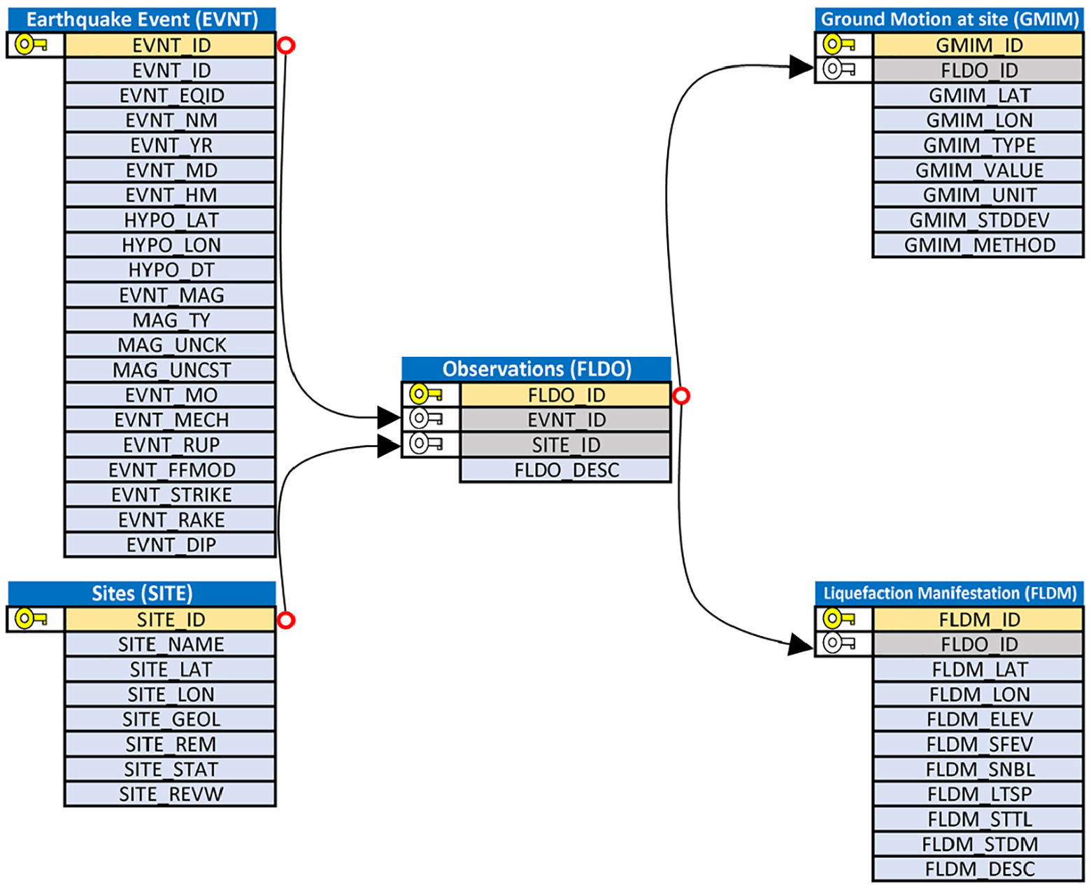
Subset of NGL relational database schema illustrating tables on post-earthquake observations of liquefaction effects.

Users may describe detailed observation(s) of site performance using the FLDM table. The location of the observation is indicated by the FLDM_LAT, FLDM_LON, and FLDM_ELEV fields. The FLDM_SFEV field indicates whether there is surface evidence of liquefaction (0 = no, 1 = yes). It is important to note that FLDM_SFEV = 0 indicates that an observation was made, and surface evidence was confirmed to have not occurred. A lack of surface evidence does not necessarily indicate a lack of liquefaction at some depth within the soil profile. Additional fields include evidence of sand boils (FLDM_SNBL), lateral spreading (FLDM_LTSP), settlement (FLDM_STTL), and structural or foundation damage (FLDM_STDM). Additional data entry options include descriptions of observations, ground displacement vectors uploaded using the FLDD table, and files such as photographs and maps of observations of damage uploaded using the FILE and FLDF tables. Minimum data requirements for the FLDM table are FLDM_LAT, FLDM_LON, and FLDM_SFEV.

Graphical user interface

The web GUI was developed using PHP: Hypertext Preprocessor, Hypertext Markup Language 5, Javascript, and Cascading Style Sheets within the CakePHP web framework. The GUI also utilizes two Application Program Interfaces (APIs) to organize the data geospatially: the Environmental Systems Research Institute Arc Geographic Information System API and the Leaflet Javascript API. The GUI can be used to visualize, upload, and download liquefaction case history data. The homepage of the database provides an overview of the geographic distribution of events, sites, and observations (Figure 4). The NGL database GUI also allows users to interact with the data by means of a list view (Figure 4b), which is convenient for seeing all of the data fields for a particular site, event, or observation in tabular form.

Figure 4.

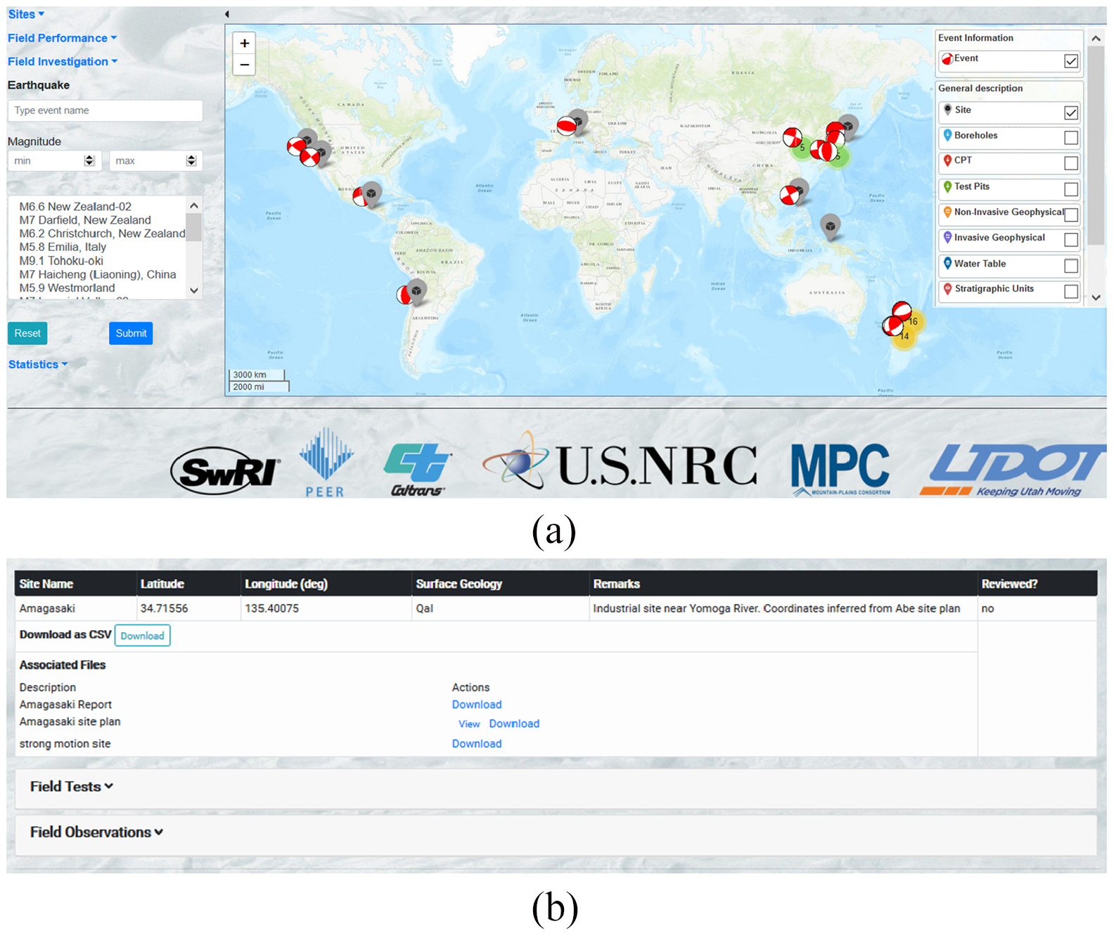
(a) Homepage of the NGL database GUI (map view) and (b) organized list of case histories in the database (list view).

In map view, users can utilize the left panel to filter the data based on earthquake name, magnitude range, or by selecting specific events from the event list. Although not shown in Figure 4, the left panel also enables filtering observed field performance by including or excluding sites that exhibited surface evidence, sand boils, lateral spreading, settlement, and/or structural damage. Case histories can also be filtered based on available field investigation information, including boreholes, CPTs, test pits, geophysical tests, and other tests. The right panel provides viewing options, including the ability to show or hide various database objects and to change the map view to topographic (default), imagery, or terrain.

Users may view site, event, and observation data through the GUI, as illustrated in Figure 5, which shows results from a CPT (CPT_21506) performed in Christchurch, New Zealand after the Canterbury earthquake sequence. The plot shows measured cone tip resistance, sleeve friction, and pore pressure. The figure is not stored in the database as an image, but rather is generated from the data when a user clicks the “Plot” button. This prevents potential inconsistencies between the data stored in the database and the figure. In a similar manner, users can plot borehole data, including stratigraphic details and SPT blow counts, shear wave velocity profiles (and dispersion curves for surface wave measurements), and observations of earthquake damage including photographs, maps, and damage descriptions.

Figure 5.

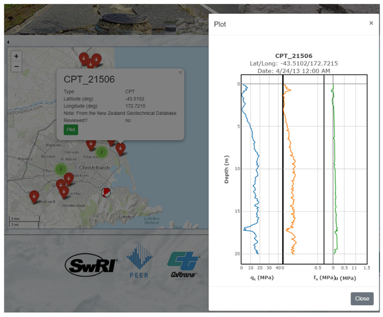
Screenshot of NGL GUI showing data for CPT_21506 in Christchurch, New Zealand.

Data review process and quality control

All data uploaded to the NGL database is reviewed using tools incorporated within the GUI. The NGL Database Working Group provides oversight to the review process. The goals of the review are to (1) ensure consistency between uploaded information and source documents; (2) verify that all required fields are provided; (3) identify ambiguities, or items that require clarification; and (4) check for reasonableness of data to identify errors in data entry such as incorrect unit conversions and inappropriate negative values. The review is intended to be objective; subjective opinions are not part of the review process. For example, a reviewer is justified in requesting clarification when data uploaded to the database do not agree with the same data plotted in a publication or other source documents. However, while a reviewer may believe that SPT data without hammer energy ratio measurements are not valuable and should not be included in development of a liquefaction model, data cannot be declined based on this subjective opinion. The NGL project has been structured in such a way that subjective judgments of this type are not made during database development, instead being reserved for the model development phase. Two independent reviewers must formally review each individual piece of information uploaded to the database.

Database population is usually performed in two steps. During the first step, users and research teams upload data, which is flagged as un-submitted and un-reviewed, and are only available to project team members in the NGL GUI. Once the user or team believes the data are ready, they submit it to the review team, at which point the data are flagged as submitted, but un-reviewed and is made available to all NGL users through the NGL GUI. After all components of a case history have been reviewed and accepted, the case history is flagged as reviewed. At this stage, users may request a DOI for their dataset. A case history is complete only if includes at least the minimum required data components, and the original source of each individual piece of information is provided. Source documents are often journal or conference publications, technical reports, theses, or dissertations. It is also possible for users to upload original (not previously published) data for which the source documents can be given as field and/or laboratory minutes or notes. In such cases, the assignment of a DOI is recommended to associate the data with the user.

Within the NGL GUI, review functions are only accessible to users having appropriate permissions. As a result, regular users are not able to access the review section of the GUI. Case history components are reviewed using three separate panels in the NGL GUI. Figure 6a shows a list of post-earthquake observations under review, while Figure 6b shows the review form for a specific observation entry in the NGL database. Similar forms are available for site information and field investigation data. The review process for an example case history and additional information on the quality control process implemented in the NGL project are provided by Zimmaro et al. (2019b).

Figure 6.

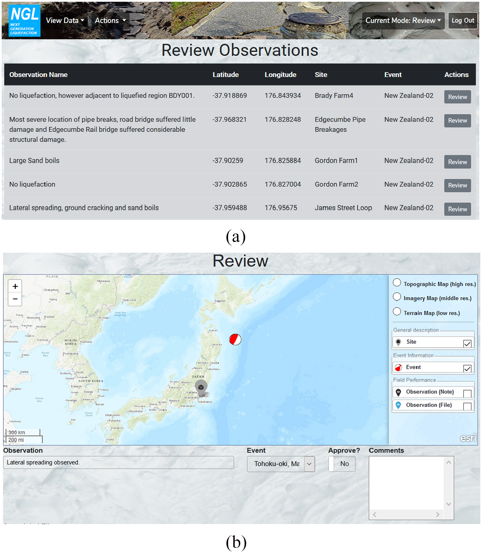
(a) Review observation panel showing post-earthquake observations under review and (b) review form for post-earthquake observations.

Cloud-based database interaction via DesignSafe

The NGL database GUI allows users to upload, visualize, and download data from the NGL database, but users cannot use the GUI to perform calculations on the data. If, for example, a user wished to compute a liquefaction index such as LPIish (Maurer et al. 2014b) for a specific CPT sounding or perform geospatial liquefaction analysis (e.g. Zhu et al., 2015, 2017), they could not do so through the GUI. One option for such analyses is to download CPT data and perform calculations on local computers. However, we anticipate that the size of the database will eventually render this approach infeasible.

To permit users to interact with the NGL database in the cloud and integrate the NGL data into their custom workflows, we periodically replicate the NGL database in DesignSafe. The significance of this replication is that users can interact with the DesignSafe version of the database via applications available through the DesignSafe Workspace, such as Jupyter notebooks, QGIS, and the Potree point cloud viewer. A Jupyter notebook is a server–client application that allows editing and running notebook documents via a web browser. It combines rich text elements (equations, figures, HTML, LaTeX) and computer code executed by a Python kernel (Pérez and Granger, 2007). These Jupyter notebooks utilize Python libraries for performing SQL queries to extract data from the database, where the extracted data may then be processed using custom computer code. Five example Jupyter notebooks that perform basic tasks that we anticipate users might perform during model development have been published in DesignSafe (Brandenberg et al., 2019b). For example, one notebook provides queries that extract various data into tables data (Brandenberg and Zimmaro, 2019a, DOI: 10.17603/ds2-xvp9-ag60.). Notebooks are also available for viewing CPT data (Brandenberg and Zimmaro, 2019b, DOI: 10.17603/ds2-99kp-rw11), boring logs and SPT data (Lee et al., 2019, DOI: 10.17603/ds2-sj7t-av93), and invasive and non-invasive geophysical test data (Zimmaro and Brandenberg, 2019, DOI: 10.17603/ds2-tq39-kp49 and Brandenberg and Zimmaro, 2019c, DOI: 10.17603/ds2-cmn0-h864).

Example SQL queries

Figure 7 shows an example SQL query that extracts CPT data at the Wildlife Array site. The query is actually a single-text string, but is broken into five lines here for clarity. The query begins on Line (6) of the Jupyter notebook, where the SELECT command queries TEST_ID, TEST_NAME, SCPT_DPTH, SCPT_RES, and SCPT_FRES. Note that data are queried from two different tables (TEST and SCPT), and the table name is prepended to the field name with a “.” separator. Line (7) utilizes an INNER JOIN command, which synthesizes two tables into a single table based on a common shared key. In this case, the SCPT and SCPG tables are combined based on a common value of SCPG_ID, which is the primary key for SCPG and a foreign key for SCPT. In line (8), another INNER JOIN adds the TEST table based on the TEST_ID key, and in line (9), the final INNER JOIN adds the SITE table based on the SITE_ID key. In line (10), the WHERE statement indicates that the requested data should be included in the query result for sites where SITE_NAME = “Wildlife Array.” The output from the query shown in Figure 7 is a small excerpt of the overall resulting data table. Note that different CPT soundings are indicated by different TEST_ID values.

Figure 7.

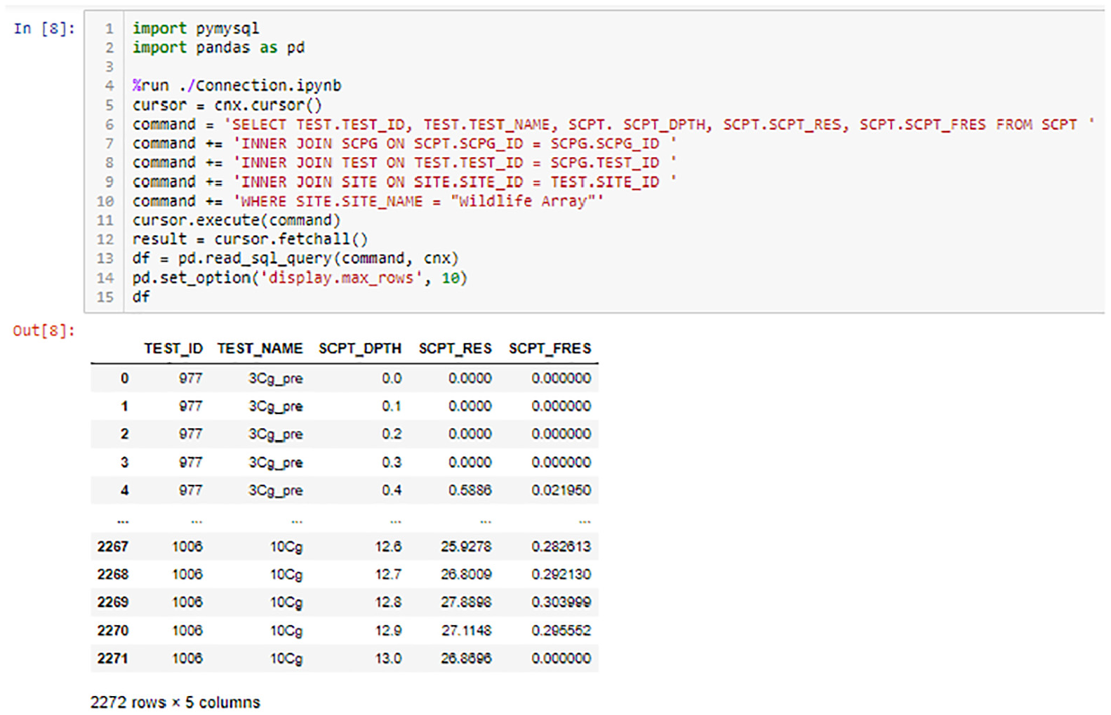
Example SQL query to extract CPT data from Wildlife Array site and output table showing truncated result.

Figure 8 shows an example query of Event and Observation data for the Wildlife Array site. In this case, the query extracts earthquake magnitude (EVNT_MAG), name (EVNT_NAME), and year (EVNT_YEAR), along with observation latitude (FLDM_LAT), longitude (FLDM_LON), whether surface evidence of liquefaction was observed (FLDM_SFEV), and a description of the observation (FLDM_DESC). 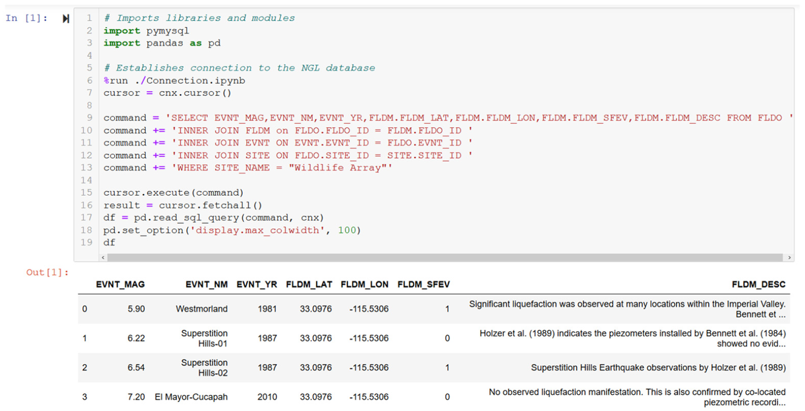Observations are available at the Wildlife Array site for four different events, two of which produced surface evidence of liquefaction (1981 M5.9 Westmorland and 1987 M6.54 Superstition Hills-02) and two of which produce no evidence of surface manifestation (1987 M6.2 Superstition Hills-01 and 2010 M7.2 El Mayor-Cucapah).

Figure 8.

Example SQL query to extract Event and Observation data from Wildlife Array site, and output table showing truncated result.

Visualization tools for geotechnical site investigation data

Figure 9 shows a Jupyter notebook for visualizing CPT data. Users select a site from a dropdown menu, and the tool populates the Test box with CPT profiles for that site. The script used to create this tool combines SITE and SCPT table entries using the INNER JOIN command. It facilitates visualization of cone tip resistance (q_c ) and sleeve friction (f_s ) for CPT profiles, along with cumulative distribution functions (CDFs) for user-specified depth ranges (full-profile or narrower depth intervals). On the right side of the visualization panel, a box labeled “Show inverse filtered data” provides a filtered q_c profile based on the Boulanger and DeJong (2018) procedure. This feature is useful for analyzing profiles with thinly interbedded soils.

Figure 9.

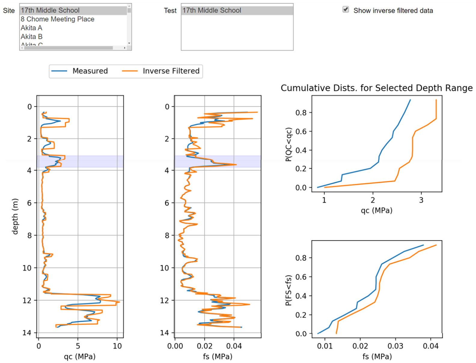
Output from the NGL CPT viewer available on DesignSafe.

Figure 10 shows a tool developed to visualize boring logs and SPT data. This tool allows users to select a site from a dropdown menu only populated with sites having boring logs and/or SPT data. This tool combines SITE, STRA, and ISPT table data entries using the INNER JOIN command. After selecting a site, the tool automatically populates the Remarks field (which shows available remarks for that site) and the TEST box with all available boring logs and SPT profiles for the site. After selecting a test, the tool plots SPT profiles (N-value versus depth) and boring logs side-to-side on the same vertical scale. The tool also plots the CDF for SPT data over user-specified depth ranges. Two additional visualization tools are available on DesignSafe: (1) a tool showing dispersion curves and inverted V_S profiles (if available) for non-invasive geophysical tests (i.e. surface wave methods) and (2) a tool showing shear wave velocity profiles and CDFs from invasive geophysical tests (e.g. cross hole, down hole, and suspension logging). The visualization tool for non-invasive geophysical tests combines SITE, GSWG, GSWD, SWVG, and SWVD table entries, while the visualization tool for invasive geophysical tests combines SITE and GIND table entries. In both cases, table entries are combined using the INNER JOIN command.

Figure 10.

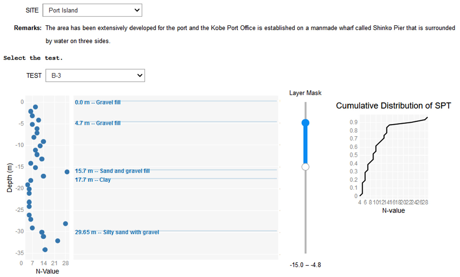
Output from the NGL SPT viewer available on DesignSafe.

Visualization tools for geospatial data

Observations of liquefaction manifestation are increasingly utilizing techniques such as LIDAR (e.g. Imakiire and Koarai, 2012; Konagai et al., 2013; Olsen et al., 2012 and Rathje et al., 2017b), SfM applied to digital photos collected using unmanned aerial vehicles (UAVs; e.g. Franke et al., 2017; Stewart et al., 2019; Winters et al., 2019), and correlation analysis of satellite images (Rathje et al., 2017b). Furthermore, geospatial products such as maps of surface geology, bodies of water, and digital elevation models provide useful information for liquefaction triggering evaluation and have been used to supplement geotechnical data in regional liquefaction assessment procedures (e.g. Zhu et al., 2015, 2017). These geospatial data objects are important to include in the NGL database.

An example application of linking geospatial data with the NGL database is provided for observations in Trona and Argus after the 2019 Ridgecrest earthquake sequence. A Geotechnical Extreme Events Reconnaissance Association (GEER) team visited these sites after the earthquakes (Stewart et al., 2019) to perform ground-based observations using GPS trackers, digital cameras, and hand-held measuring devices, and subsequently a team visited these sites to fly UAVs and gather image data. Data from these reconnaissance missions were published in DesignSafe (Brandenberg et al., 2019a; Winters et al., 2019) and assigned DOIs that are included as citations in the CITATION table and linked to the observation through the FLDP table. Orthomosaic images obtained from the UAV survey (Winters et al., 2019) are superposed on a surface geology map (Smith, 2009) using QGIS in DesignSafe in Figure 11. Three different orthomosaics are shown, and a zoomed-in view of one orthomosaic shows a railroad that required repair due to liquefaction effects near the intersection of three different geologic units (sdg (gravel and sand), oal (older alluvium), and sd (sand and silt)).

Figure 11.

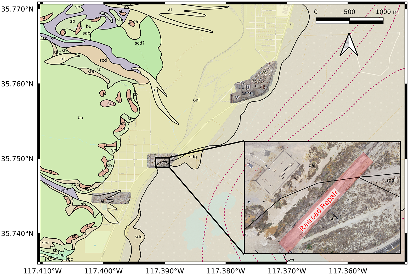
Map of Trona and Argus where liquefaction effects were observed after the Ridgecrest earthquake sequence. The map includes orthomosaic images obtained from UAV SfM surveys (Winters et al., 2019), and a surface geology map by Smith (2009).

A point cloud generated by SfM processing of the UAV images shows surface evidence of liquefaction at the site of the Family Dollar store in Trona, CA in Figure 12. The image is a screenshot from the Potree point cloud viewer available in DesignSafe. Sand ejecta originating from a utility pole near the left side of the image flowed over the gravel and parking lot toward the sign on the right of the image.

Figure 12.

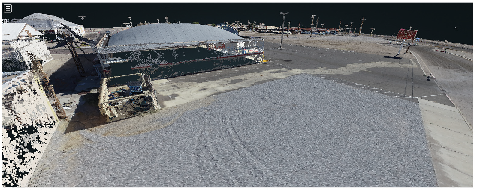
Point cloud from SfM processing of UAV images at the Family Dollar building in Trona, CA (Winters et al., 2019).

Conclusion

In this article, we present the NGL database (Zimmaro et al., 2019a, DOI: 10.21222/C2J040). The NGL database is an open-source tool that results from a multi-year, ongoing community effort. We describe the NGL database organizational structure (i.e. the schema describing relationships among tables) and provide information about selected tables in the database, including minimum data requirements. The NGL database contains objective information about liquefaction, or lack thereof, during past earthquake events. Each individual site and observation component is reviewed through a formal vetting process coordinated by the NGL Database Working Group.

The NGL database is accessible through a GUI that allows users to upload, visualize, and download data. The database is also replicated onto DesignSafe where users can write queries and utilize Jupyter notebooks to interact with the data in the cloud and integrate geospatial data into their workflow. We envision these cloud-based tools to be particularly useful for data analysis in support of development of future liquefaction susceptibility, triggering, and consequences models.

Footnotes

Acknowledgements

The authors acknowledge the contributors of datasets, input on the schema during workshops, and/or input during database working group meetings by Russel Green and Kristin Ulmer (Virginia Tech); Ross Boulanger (UC Davis); Robert Kayen (USGS/UC Berkeley); Kyle Rollins (BYU); Sjoerd van Ballegooy and Mike Liu (Tonkin + Taylor); Mike Greenfield (Greenfield Geotechnical); Christine Beyzaei and Sean Ahdi (Exponent); Jonathan Bray (UC Berkeley); James Gingery (Hayward Baker); Eric Thompson (USGS); Yousef Bozorgnia (UCLA); Miriam Juckett (SwRI); Roy Mayfield (Consulting Engineer); Steve Bartlett and Massoud Hosseinali (University of Utah); Mahyar Sharifi-Mood, Tim Cockerill, Christopher Jordan, and Steve Mock (Texas Advanced Computing Center); Ellen Rathje, Maria Giovanna Durante, and Michael Little (University of Texas); Laurie Baise (Tufts University); Silas Nichols (FHWA); Derrick Wittwer (Bureau of Reclamation); Ahmed Elgamal (UCSD); Lelio Mejia (Geosyntec); Robert Pyke (Consulting Engineer); Albert Kottke (PG&E); Yi Tyan Tsai (GeoEngineers Inc.); Tom Shantz (Caltrans); Zia Zafir (Kleinfelder); Esam Abraham (Southern California Edison); Khaled Chowdhuri (USACE); Harold Magistrale (FM Global); Marty Hudson (Wood); Jianping Hu (LADWP); Craig Davis (recently retired LADWP); Joseph Weber (Loyola Marymount University); Tim Ancheta (RMS); Ariya Balakrishnan (California Division of Safety of Dams); and Allison Lee, Honor Fisher, Omar Issa, Wyatt Iwanaga, Arielle Sanghvi, Christopher Nicas, Jared Rivera, Michael A. Winders, Naoto Inagaki, Sahil Sibal, Siddhant Jain, Trini Inouye, Bryan Ong, Anjali Swamy, Tristan Buckreis, and Chukwuebuka Nweke (UCLA). The web-based graphical user interface was developed by Joey Mukherjee, Zachary Murphy, and Steven Ybarra (SWRI).

Declaration of conflicting interests

The author(s) declared no potential conflicts of interest with respect to the research, authorship, and/or publication of this article.

Funding

The author(s) disclosed receipt of the following financial support for the research, authorship, and/or publication of this article: Financial support for the NGL project is provided by California Department of Transportation (Caltrans) through the Pacific Earthquake Engineering Research Center (PEER) and by the US Nuclear Regulatory Commission (NRC) through the Southwest Research Institute (SWRI). Neither the US Government nor any agency thereof, nor any of their employees, makes any warranty, expressed or implied, or assumes any legal liability or responsibility for any third party’s use, or the results of such use, of any information, apparatus, product, or process disclosed in this paper, or represents that its use by such third party would not infringe privately owned rights. The views expressed in this paper are not necessarily those of the US Nuclear Regulatory Commission.

ORCID iD

Scott J. Brandenberg

References

Andrus

Stokoe

II (2000) Liquefaction resistance of soils from shear-wave velocity. Journal of Geotechnical & Geoenvironmental Engineering 126(11): 1015–1025.

Boulanger

DeJong

(2018) Inverse filtering procedure to correct cone penetration data for thin-layer and transition effects. In: Proceedings of the 4th international symposium on cone penetration testing (CPT’18), Delft, 21–22 June.

Boulanger

Idriss

(2012) Probabilistic standard penetration test-based liquefaction-triggering procedure. Journal of Geotechnical & Geoenvironmental Engineering 138: 1185–1195.

Boulanger

Idriss

(2016) CPT-based liquefaction triggering procedure. Journal of Geotechnical & Geoenvironmental Engineering 142(2): 04015065.

Bozorgnia

Abrahamson

Al Atik

, et al. (2014) NGA-West2 research project. Earthquake Spectra 30: 973–987.

Bozorgnia

Stewart

Abrahamson

, et al. (2020). Chapter 1: Introduction, in Data Resources for NGA-Subduction Project, Stewart

J.P.

(editor), Report PEER 2020/02, Pacific Earthquake Engineering Research Center, UC Berkeley (headquarters).

Brandenberg

Zimmaro

(2019a) Next Generation Liquefaction (NGL) Partner Dataset—Cone Penetration Test (CPT) Viewer, DesignSafe-CI, Dataset. DOI: 10.17603/ds2-99kp-rw11.

Brandenberg

Zimmaro

(2019b) Next Generation Liquefaction (NGL) Partner Dataset—Sample Queries, DesignSafe-CI, Dataset. DOI: 10.17603/ds2-xvp9-ag60.

Brandenberg

Zimmaro

(2019c) Next Generation Liquefaction (NGL) Partner Dataset—Surface Wave Viewer, DesignSafe-CI, Dataset. DOI: 10.17603/ds2-cmn0-h864.

10.

Brandenberg

Goulet

Wang

, et al. (2019a) Ridgecrest, CA earthquake sequence, July 4 and 5, 2019. DesignSafe-CI. DOI: 10.17603/ds2-4thk-d514.

11.

Brandenberg

Kwak

Zimmaro

, et al. (2018) Next-Generation Liquefaction (NGL) case history database structure. In: Fifth decennial GEESD conference (Geotechnical Special Publication), Austin, TX, 10–13 June, vol. 290, pp. 426–433. Reston, VA: American Society of Civil Engineers.

12.

Brandenberg

Zimmaro

Lee

, et al. (2019b) Next Generation Liquefaction (NGL) Partner Dataset, DesignSafe-CI, Dataset. DOI:10.17603/ds2-2xzy-1y96.

13.

Çetin

Seed

Der Kiureghian

, et al. (2004) SPT-based probabilistic and deterministic assessment of seismic soil liquefaction potential. Journal of Geotechnical & Geoenvironmental Engineering 130(12): 1314–1340.

14.

Çetin

Seed

Kayen

, et al. (2018) SPT-based probabilistic and deterministic assessment of seismic soil liquefaction triggering hazard. Soil Dynamics and Earthquake Engineering 115: 698–709.

15.

Cubrinovski

Rhodes

Ntritsos

Van Ballegooy

(2019) System response of liquefiable deposits. Soil Dynamics and Earthquake Engineering 124: 212–229.

16.

Foti

Hollender

Garofalo

, et al. (2018) Guidelines for the good practice of surface wave analysis: A product of the InterPACIFIC project. Bulletin of Earthquake Engineering 16: 2367–2420.

17.

Franke

Rollins

Ledezma

, et al. (2017) Reconnaissance of two liquefaction sites using small unmanned aerial vehicles and structure from motion computer vision following the April 1, 2014 Chile earthquake. Journal of Geotechnical & Geoenvironmental Engineering 143(5): 04016125.

18.

Goulet

Bozorgnia

Abrahamson

, et al. (2018) Central and Eastern North America Ground—Motion Characterization—NGA-East Final Report (PEER Report 2018/08). Berkeley, CA: Pacific Earthquake Engineering Research Center.

19.

Greenfield

(2017) Effects of long-duration ground motions on liquefaction hazards. PhD Dissertation, University of Washington, Seattle, WA.

20.

Imakiire

Koarai

(2012) Wide-area land subsidence caused by the 2011 off the Pacific Coast of Tohoku earthquake. Soils and Foundations 52: 842–855.

21.

Kayen

Moss

RES

Thompson

, et al. (2013) Shear-wave velocity–based probabilistic and deterministic assessment of seismic soil liquefaction potential. Journal of Geotechnical & Geoenvironmental Engineering 139: 407–419.

22.

Konagai

Kiyota

Suyama

, et al. (2013) Maps of soil subsidence for Tokyo bay shore areas liquefied in the March 11th, 2011 off the Pacific Coast of Tohoku earthquake. Soil Dynamics and Earthquake Engineering 53: 240–253.

23.

Kramer

Mitchell

(2006) Ground motion intensity measures for liquefaction hazard evaluation. Earthquake Spectra 22: 413–438.

24.

Kramer

Sideras

Greenfield

(2016) The timing of liquefaction and its utility in liquefaction hazard evaluation. Soil Dynamics and Earthquake Engineering 91: 133–146.

25.

Kwak

Stewart

Brandenberg

, et al. (2016) Characterization of seismic levee fragility using field performance data. Earthquake Spectra 32: 193–215.

26.

Lee

Fisher

Zimmaro

, et al. (2019) Next Generation Liquefaction (NGL) Partner Dataset—Boring Log Viewer, DesignSafe-CI, Dataset. DOI: 10.17603/ds2-sj7t-av93.

27.

Lewis

Arango

Kimball

, et al. (1999) Liquefaction resistance of old sand deposits. In: Proceedings of the 11th PanAmerican conference on soil mechanics and geotechnical engineering, Foz do Iguassu, Brasil, 8–12 August, pp. 821–829. London: ISSMGE [International Society for Soil Mechanics and Geotechnical Engineering]

28.

Maurer

Green

Taylor

O-DS

(2014a) Moving towards an improved index for assessing liquefaction hazard: Lessons from historical data. Soils and Foundations 55: 778–787.

29.

Maurer

Green

Cubrinovski

, et al. (2014b) Evaluation of the liquefaction potential index for assessing liquefaction hazard in Christchurch, New Zealand. Journal of Geotechnical and Geoenvironmental Engineering 140: 04014032.

30.

Moss

RES

Seed

Kayen

, et al. (2006) CPT-based probabilistic and deterministic assessment of in situ seismic soil liquefaction potential. Journal of Geotechnical & Geoenvironmental Engineering 132: 1032–1051.

31.

National Academies of Sciences, Engineering, and Medicine (2016) State of the Art and Practice in the Assessment of Earthquake-Induced Soil Liquefaction and Its Consequences. Washington, DC: The National Academies Press.

32.

Obermeier

Jacobson

Smoot

, et al. (1990) Earthquake-Induced Liquefaction Features in the Coastal Setting of South Carolina and in the Fluvial Setting of the New Madrid Seismic Zone (U.S. Geological Survey professional paper 1504). Washington, DC: U.S. Government Printing Office.

33.

Olsen

Cheung

Yamazaki

, et al. (2012) Damage assessment of the 2010 Chile earthquake and tsunami using terrestrial laser scanning. Earthquake Spectra 28(Suppl. 1): S179–S197.

34.

Pérez

Granger

(2007) IPython: A system for interactive scientific computing. Computing in Science and Engineering 9(3): 21–29.

35.

Rathje

Dawson

Padgett

, et al. (2017a) DesignSafe: A new cyberinfrastructure for natural hazards engineering. Natural Hazards Review 18(3): 06017001-1–06017001-7.

36.

Rathje

Secara

Martin

, et al. (2017b) Liquefaction-induced horizontal displacements from the Canterbury earthquake sequence in New Zealand measured from remote sensing techniques. Earthquake Spectra 33: 1475–1494.

37.

Robertson

Wride

(1998) Evaluating cyclic liquefaction potential using the cone penetration test. Canadian Geotechnical Journal 35(3): 442–459.

38.

Seed

Idriss

Arango

(1983) Evaluation of liquefaction potential using field performance data. Journal of Geotechnical & Geoenvironmental Engineering 109(3): 458–482.

39.

Smith

(2009) Late Cenozoic Geology and Lacustrine History of Searles Valley, Inyo and San Bernardino Counties (Professional paper 1727). Menlo Park, CA: U.S. Geological Survey.

40.

Stafford

(2012) Evaluation of structural performance in the immediate aftermath of an earthquake: A case study of the 2011 Christchurch earthquake. International Journal of Forensic Engineering 1: 58–77.

41.

Stewart

(ed.), Brandenberg

Wang

, et al. (2019) Preliminary Report on Engineering and Geological Effects of the July 2019 Ridgecrest Earthquake Sequence (Report GEER-064). Geotechnical Extreme Events Reconnaissance Association. DOI: 10.18118/G6H66K

42.

Stewart

Kramer

Kwak

, et al. (2016) PEER-NGL project: Open source global database and model development for the next-generation of liquefaction assessment procedures. Soil Dynamics and Earthquake Engineering 91: 317–328.

43.

van Ballegooy

Malan

Lacrosse

, et al. (2014) Assessment of liquefaction-induced land damage for residential Christchurch. Earthquake Spectra 30: 31–55.

44.

Winters

Delisle

M-PC

Lucey

JTD

, et al. (2019) UCLA UAV Imaging in Ridgecrest, CA Earthquake Sequence, July 4 and 5, 2019, DesignSafe-CI, Dataset. DOI: 10.17603/ds2-wfgc-a575.

45.

Youd

Hoose

(1978) Historic Ground Failures in Northern California Triggered by Earthquakes (Professional paper 993). U.S. Geological Survey. Available at: http://pubs.usgs.gov/pp/1978/pp0993/ (accessed December 2019).

46.

Youd

Perkins

(1978) Mapping liquefaction-induced ground failure potential. Journal of the Geotechnical Engineering Division 104(4): 433–446.

47.

Zhu

Baise

Thompson

(2017) An updated geospatial liquefaction model for global application. Bulletin of the Seismological Society of America 107: 1365–1385.

48.

Zhu

Daley

Baise

, et al. (2015) A geospatial liquefaction model for rapid response and loss estimation. Earthquake Spectra 31: 1813–1837.

49.

Zimmaro

Brandenberg

(2019) Next Generation Liquefaction (NGL) Partner Dataset—Invasive Geophysical Test Viewer, DesignSafe-CI, Dataset. DOI: 10.17603/ds2-tq39-kp49.

50.

Zimmaro

Brandenberg

Bozorgnia

, et al. (2019b) Quality control for next-generation liquefaction case histories. In: VII international conference on earthquake geotechnical engineering (ed Silvestri

Moraci

, Earthquake Geotechnical Engineering for Protection and Development of Environment and Constructions), Rome, Italy, 17–20 June, pp. 5905–5912. Italy: Associazione Geotecnica Italiana.

51.

Zimmaro

Brandenberg

Stewart

, et al. (2019a) Next-Generation Liquefaction Database. Next-Generation Liquefaction Consortium. DOI: 10.21222/C2J040