Study on normalization of residual displacements for single-degree-of-freedom systems

Abstract

Residual displacement spectrum is one of the most important means to predict the permanent deformation of structures after the earthquake, and various normalizations of residual displacements have generally been used for construction of the spectrum. However, the issue regarding the merits and drawbacks of each normalization has not yet been investigated thoroughly. A comparison between two normalizations that relate the residual displacements to the elastic and inelastic displacements is made in terms of the effect of ground motion and structural characteristics by means of the results of nonlinear time history analysis. The statistical results reveal that the residual-to-peak-inelastic displacement ratios have the advantages of small dispersion, samples without any outliers, and relatively symmetric distribution, which benefits from the strong correlation between residual and peak inelastic displacements. Moreover, the residual-to-peak-inelastic displacement ratios are almost independent of site conditions, significant duration, and natural periods. Consequently, the peak inelastic displacements are superior to the elastic ones as an intermediate step for residual displacements estimation, provided that the peak inelastic displacements are estimated with a low uncertainty. For providing alternatives to estimate residual displacement demands, the constant-strength residual displacement spectra are developed for both normalizations.

Keywords

SDOF systems residual displacements normalization linear correlation constant-strength residual displacement spectra

Introduction

Past earthquake reconnaissance observations (Eguchi et al., 1998; Fujino et al., 2005; Paterson et al., 2008; Ramirez and Miranda, 2012) show that the total economic losses during a damaging earthquake event include not only the direct losses associated with demolition and reconstruction of the collapsed buildings but also the indirect losses related to the costs of repairing, and even removing and rebuilding the lifelines and other essential infrastructures without collapsing but sustaining certain permanent deformations. In particular, the economic losses at the intermediate levels of ground motion intensity are often dominated by losses due to residual drifts (Ramirez and Miranda, 2012). Therefore, in addition to the collapse prevention, sufficient attention should also be paid to the post-earthquake reparability of structures. The former is mainly controlled by the peak inelastic displacement, while the latter generally uses the residual displacement as an important criterion. For example, after the 1995 Kobe earthquake (Fujino et al., 2005), as many as 88 single reinforced concrete (RC) piers were forced to replace or remove simply because of the excessive permanent deformation resulting in technical difficulties and elevated costs.

Recognizing the importance of controlling residual displacements, several investigations have focused on assessing the factors influencing the residual displacement demands, and some empirical equations have also been proposed to estimate the residual displacement demands of structures that can be simplified to single-degree-of-freedom (SDOF) systems. Mahin and Bertero (1981) found that for elastoplastic systems, the mean residual displacements are more than 40% of the peak inelastic displacements. Moreover, the coefficients of variation (COVs) of the residual displacements are nearly twice the value associated with the peak inelastic displacements. MacRae and Kawashima (1997) and Kawashima et al. (1998) statistically analyzed the residual displacements normalized by the maximum possible residual displacements of bilinear oscillators, respectively, subjected to 11 and 63 ground motions and then proposed a residual displacement spectrum to be used in the design of new bridge piers in Japan (Japan Road Association, 2002). Borzi et al. (2001) assessed the effect of the softening behavior (negative post-yield stiffness) on the ratios of residuals to peak inelastic displacements for the elastoplastic model. Christopoulos et al. (2003) investigated the effect of hysteretic characteristics, post-yield stiffness as well as maximum ductility on the residual displacements normalized by peak inelastic displacements for four SDOF oscillators representative of RC frame buildings with different stories. To facilitate the estimation of residual displacement demands, a simplified equation for the elastoplastic system was proposed by Ruiz-García and Miranda (2006b), where the residual displacements were normalized by the elastic spectral displacements. Liossatou and Fardis (2015, 2016) examined the influence of near-fault ground motions with and without distinct velocity pulses on the residual displacements of SDOF systems having various hysteretic rules representing a range of typical RC structures. The authors found that the residual displacements came out on average equal to about a constant fraction of the peak inelastic displacements, regardless of the presence of a velocity pulse in the ground motions. Recently, Guerrero et al. (2017), Ji et al. (2018), and Ruiz-García and Guerrero (2017) studied the residual displacements normalized by the elastic spectral ones for SDOF systems subjected to ground motions recorded at soft-soil sites. The spectral trend of residual displacement ratios for the soft-soil sites was found to be different from the spectral trend for firm sites. Particularly, residual displacement ratios significantly decrease when the natural period is close, or equal, to the predominant period of the ground motion recorded in soft-soil site. Very recently, Quinde et al. (2020) developed a simplified relation between the residual and peak inelastic displacement demands for soft soils. For estimation of the residual displacements of structures under the mainshock-aftershock sequences, an average residual displacement spectrum was proposed by Amiri and Bojórquez (2019), where the residual displacements were normalized with respect to the elastic spectral ones. Girija and Gupta (2020) conducted a comprehensive statistical estimation of residual displacement spectrum via normalization with respect to inelastic and elastic spectral displacements, and the expressions were proposed for both types of normalization.

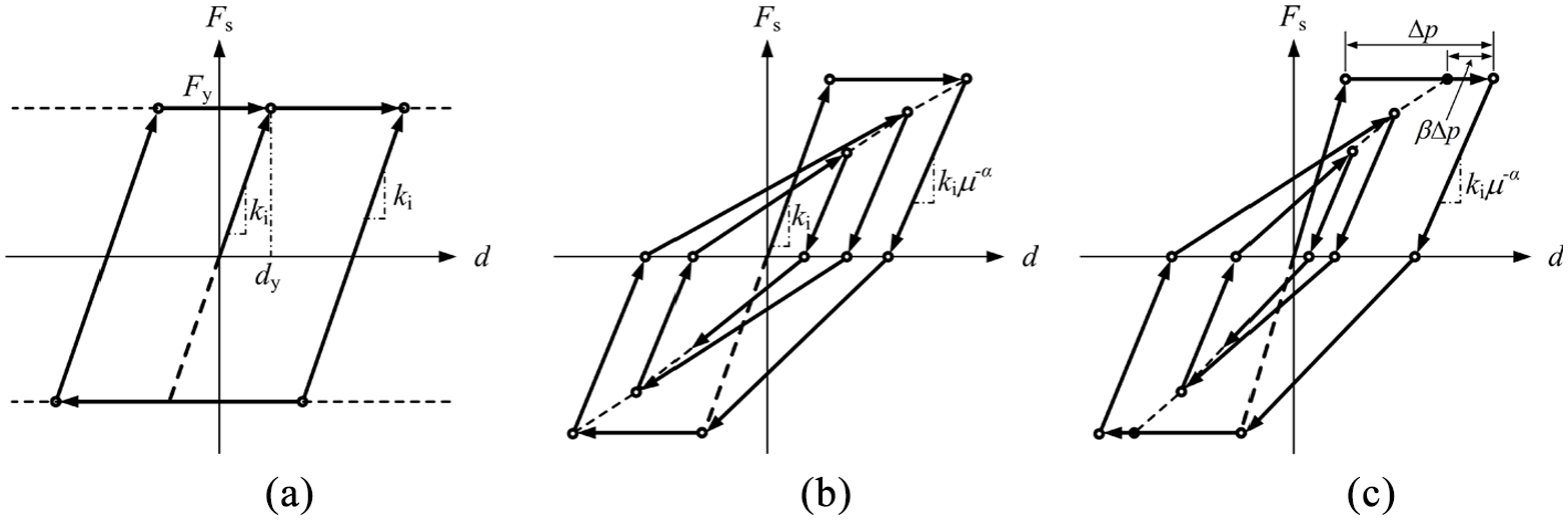
From the literature survey, it is apparent that the average response spectrum has been recognized as one of the most important means to estimate the residual displacement demands to date, and mainly three different definitions of the residual displacement ratios were used in construction of the spectra, that is, the residual displacements normalized with respect to the maximum possible residual displacements (d_r,m, quasi-statically unloading from the peak inelastic displacement to the line of zero lateral force), elastic spectral displacements (S_d), and peak inelastic displacements (d_m), respectively. As a matter of fact, the use of various definitions of residual ratios will inevitably result in discrepancies in terms of both simplicity and accuracy in the estimation of residual displacement demands. For instance, the maximum possible residual displacements as the upper limit of residual displacements cannot be always obtained simply by linear quasi-static unloading from the peak inelastic displacements and the extra computational burden will be introduced, such as nonlinear response of structures having bilinear Takeda hysteretic rules with negative reloading stiffness parameters, or structures having smooth hysteretic models (e.g. BWBN and Ramberg–Osgood), as illustrated in Figure 1. Furthermore, the maximum possible residual displacements are unnecessary in the routine seismic design process. As a result, such normalization will evidently lead to a redundant procedure and is not recommended for residual displacements estimation. Note, however, that most of the existing studies generally state the residual displacement demands to be normalized by a certain displacement demand. The pros and cons of each normalization format used in residual displacement demands estimation have not yet been systematically reported.

Figure 1.

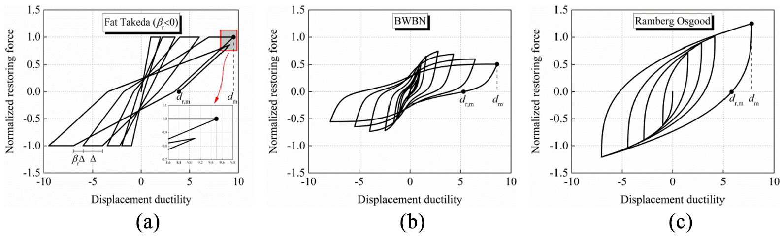
(a) Takeda hysteretic model with negative reloading stiffness parameter, (b) BWBN model, and (c) Ramberg–Osgood model.

The objective of this article is to investigate the impact of the choice of normalization parameters on residual displacements estimation. Meanwhile, the merits and drawbacks of different types of normalization used for estimation are analyzed. For these purposes, the residuals are, respectively, normalized by elastic spectral and peak inelastic displacements. A comparison of the effect of local site conditions, ground motion durations, natural periods, yield strength reduction factors, and hysteretic rules on two different definitions of residual displacement ratios is made by means of the results of nonlinear time history analysis (NTHA) under 240 ground motions. The constant-strength residual displacement spectra, which allow the estimation of residual displacement demands in terms of both elastic spectra and peak inelastic displacements, are finally constructed for three typical hysteretic models.

Earthquake ground motions

To obtain the post-earthquake residual displacement demands, an ensemble of 240 earthquake records drawn from the Ground Motion Database of the Pacific Earthquake Engineering Research Center (PEER, 2019) was used as seismic input in this study. All ground motions satisfy the following requirements: (1) surface-wave magnitudes (M_s) are greater than or equal to 5.0; (2) gathered from rock or firm sites with average shear-wave velocities (v_s,30) greater than 180 m/s in the upper 30 m of the site profile; (3) at least one of the two horizontal components has a peak ground acceleration (PGA) larger than 20 cm/s²; and (4) without velocity pulse characteristics or directivity effects. Details of all ground motion records can be found in Feng and Gong (2020).

In accordance with the site classification specified in FEMA-450 (Federal Emergency Management Agency (FEMA), 2003), the records considered in this study were divided into three groups. Each contains 80 ground motions, corresponding to rock with 760 m/s < v_s,30 ≤ 1500 m/s (site class B), very dense soil and soft rock with 360 m/s < v_s,30 ≤ 760 m/s (site class C), and stiff soil with 180 m/s < v_s,30 ≤ 360 m/s (site class D), respectively. The ranges of M_s are 5.3–7.6, 5.1–7.4, and 5.0–7.4, respectively, for site classes B, C, and D, and the average PGA for each site class is 72.33, 147.16, and 114.33 cm/s².

Figure 2 shows the average elastic response spectra, where the spectral ordinates are computed for each earthquake record and then averaged for different components. Note that the ground acceleration of each record is divided by its PGA, which anchors the zero-period ordinate for a standard spectral shape. Evidently, the shapes of the spectra for three site groups are different in terms of the predominant periods (the period at which the maximum spectral acceleration amplitude is concentrated) and the spectral acceleration amplitudes. Figure 3 depicts the distribution of distances to horizontal projection of rupture (R_rup), surface-wave magnitudes (M_s), and peak ground accelerations (PGA) for all ground motions considered in this study. The R_rup ranges from 2.9 to 151.1 km and the PGA ranges from 15.26 to 645.38 cm/s². About 90% ground motions were recorded from earthquake events having M_s greater than 5.5. To have a look at the distribution of ground motion duration, the significant duration defined by Trifunac and Brady (1975) is computed for all ground motions, and the histogram is presented in Figure 4. The significant duration ranges from 3.5 to 35.1 s, 2.4 to 36.4 s, and 3.8 to 34.9 s, respectively, for site classes B, C, and D. Since the dataset considered in this study does not include far-field long-duration ground motions or enough motions from large-magnitude earthquakes, the findings as well as the response spectra developed in this study cannot be reliably applied to these extreme cases.

Figure 2.

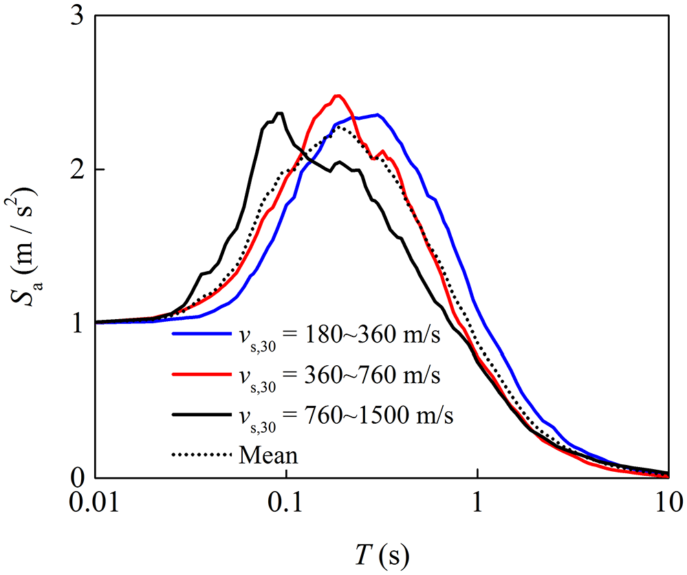
Average elastic acceleration response spectra with 5% damping ratio.

Figure 3.

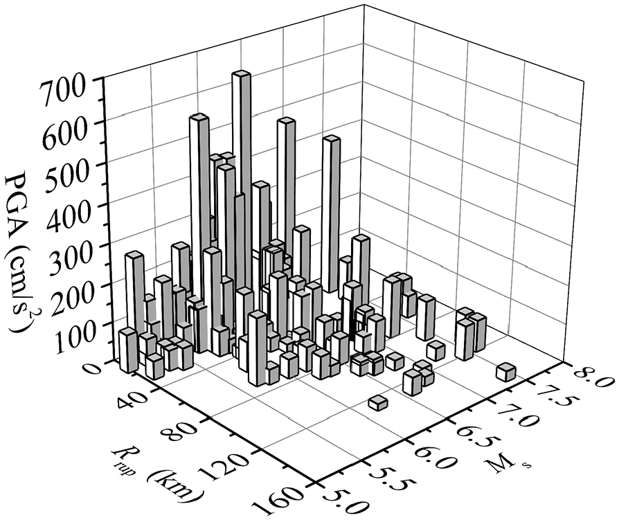
Distribution of R_rup-M_s-PGA for all ground motions.

Figure 4.

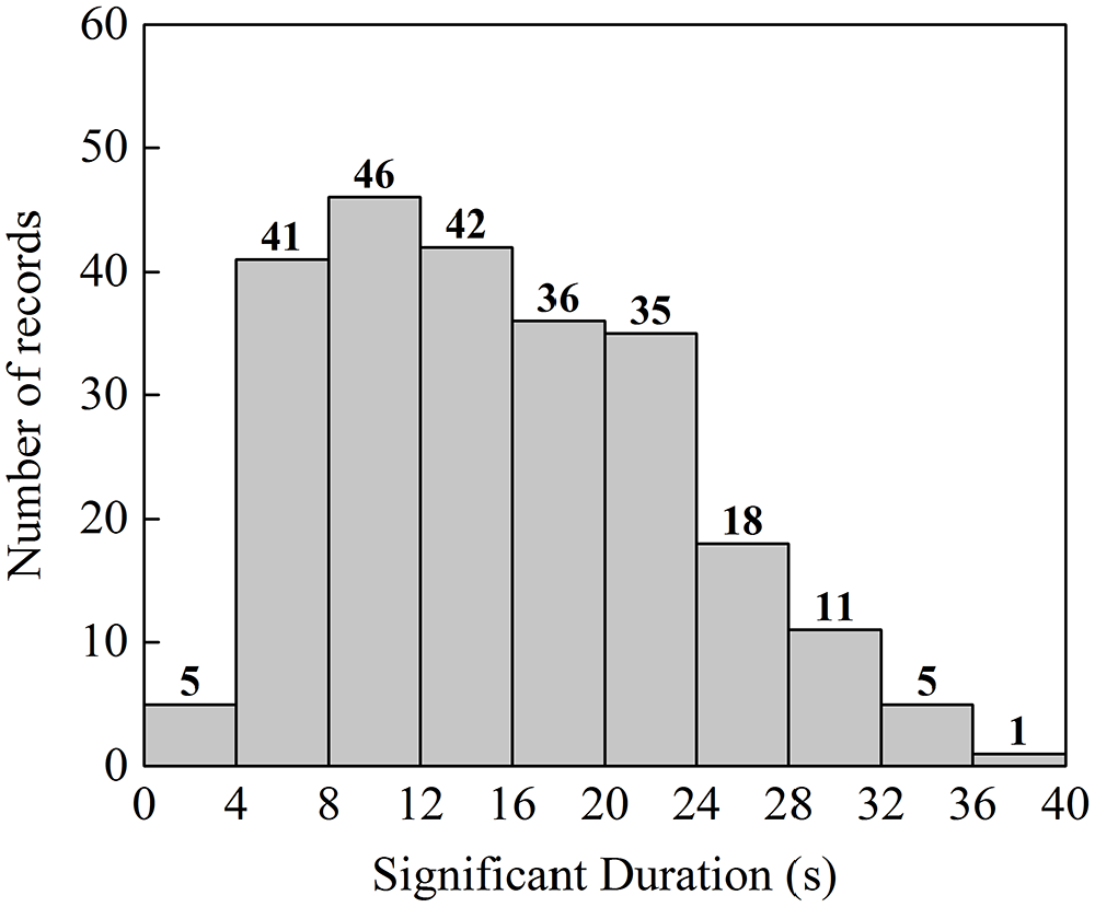
Histogram of significant duration.

Hysteretic models

The hysteretic rules have been demonstrated to be one of the most important factors affecting the residual displacement demands (Christopoulos et al., 2003; Dazio, 2004; Liossatou and Fardis, 2015). In view of this, three typical hysteretic models were selected for this study as illustrated in Figure 5. The elastoplastic model in Figure 5a can be considered an adequate approximation to the steel-framed structures and seismic isolation systems. The Thin Takeda (Otani, 1974) and Fat Takeda (Kanaan and Powell, 1973) models in Figure 5b and c represent a range of hysteresis shapes appropriate for RC and reinforced masonry structures. The former is a representative of RC members with significant axial load, such as building columns, bridge column piers, and walls (Priestley et al., 2007) and can also be used elsewhere for simulation of nonlinear dynamic behaviors of rubble-stone masonry structures (Ali et al., 2013). For this model, the unloading stiffness degrading factor (as defined in the figure) α = 0.3 is assumed as a typical value of these structures. The latter, who incorporates the former as a special case, is a representative of a series of RC beams. For well-detailed beams, the parameters α = 0.3 and β = 0.6 are generally considered to be appropriate.

Figure 5.

Hysteretic models used in this study: (a) elastoplastic, (b) thin Takeda, and (c) fat Takeda.

Analysis methodology

Residual displacement ratios

To investigate the impact of the choice of normalization formats on the residual displacement estimation, the residual displacement demands are normalized by two different displacements in this study, respectively, defined as follows:

C_{e} = \frac{d_{r}}{S_{d}}

(1)

and

C_{p} = \frac{d_{r}}{d_{m}}

(2)

where S_d is the elastic spectral displacement under an acceleration time history; d_m and d_r are the peak inelastic displacement and the residual displacement, respectively, computed using NTHA of SDOF systems with constant relative lateral strength subjected to the same acceleration time history. The relative lateral strength is measured by the yield strength reduction factor, R, which is defined as

R = \frac{m S_{a}}{F_{y}}

(3)

where m and F_y are the mass and the yield strength of the structures, respectively; S_a is the elastic spectral pseudo-acceleration.

Initial viscous damping models

The NTHA has already been widely used for describing the behavior of structures under seismic actions. It is apparent that the reliability of NTHA results is largely dependent on the modeling choice, of which the modeling of viscous damping forces is a crucial aspect. To date, a great deal of research has been carried out focusing on this topic (Charney, 2008; Chopra and McKenna, 2016; Hall, 2006, 2017; Hardyniec and Charney, 2015, 2017; Jehel et al., 2014; Petrini et al., 2008; Priestley and Grant, 2005; Smyrou et al., 2011). However, even for simple SDOF systems, the modeling of damping forces is still controversial.

The initial-stiffness proportional damping (ISPD), also termed the mass proportional damping, was shown to produce unrealistically high amount of damping energy dissipation (Priestley and Grant, 2005) and large damping forces (Hall, 2006), thus resulting in an analytical results being unconservative.

The tangent-stiffness proportional damping (TSPD), advocated by Priestley and Grant (2005), was demonstrated to effectively eliminate such unrealistic response quantities. Nevertheless, this model was criticized for lacking a physical basis and having conceptual issues (Chopra and McKenna, 2016; Hall, 2006, 2017). However, in analyses performed by Hardyniec and Charney (2017), no detrimental influences associated with the conceptual issues were observed. Furthermore, the shake-table tests (Otani, 1980; Petrini et al., 2008) confirmed that TSPD provided the best agreement with the experimental observations, while ISPD would result in an underestimation of the displacement demand. Hence, the TSPD assumption has been implemented by many researchers for NTHA. In this work, the TSPD with a damping ratio of 5% was used in nonlinear dynamic analysis.

Analytical parameters

Two different residual displacement ratios, C_e and C_p as defined in Equations 1 and 2, were computed for SDOF systems having a set of 30 natural periods (T, from 0.1 to 3.0 s), three hysteretic rules (elastoplastic, Thin Takeda, and Fat Takeda), and 10 levels of yield strength reduction factors (R, from 1.5 to 10) when subjected to an ensemble of 240 ground motions recorded at three different firm sites.

Correlation analysis

Before making a comparison between two methodologies that relate the residual displacements with the elastic and inelastic displacement demands, it is desirable to first look at the correlation between residuals and each of these two intermediate demands. To this end, the residual displacement d_r, elastic spectral displacement S_d, and peak inelastic displacement d_m are computed for each of 240 ground motions.

As an example, Figure 6 shows the scatter plots of d_r versus S_d and d_r versus d_m for elastoplastic systems with typical combinations of T and R. Note that the d_r, S_d, and d_m are, respectively, normalized by their maximum values max(d_r), max(S_d), and max(d_m), which allows all subplots to have the same scales. A comparison of Figure 6a and b suggests that the residual displacements have a better linear relation with the peak inelastic displacements. This reveals that the structures undergoing large peak inelastic displacements are more prone to sustain excessive residual displacements.

Figure 6.

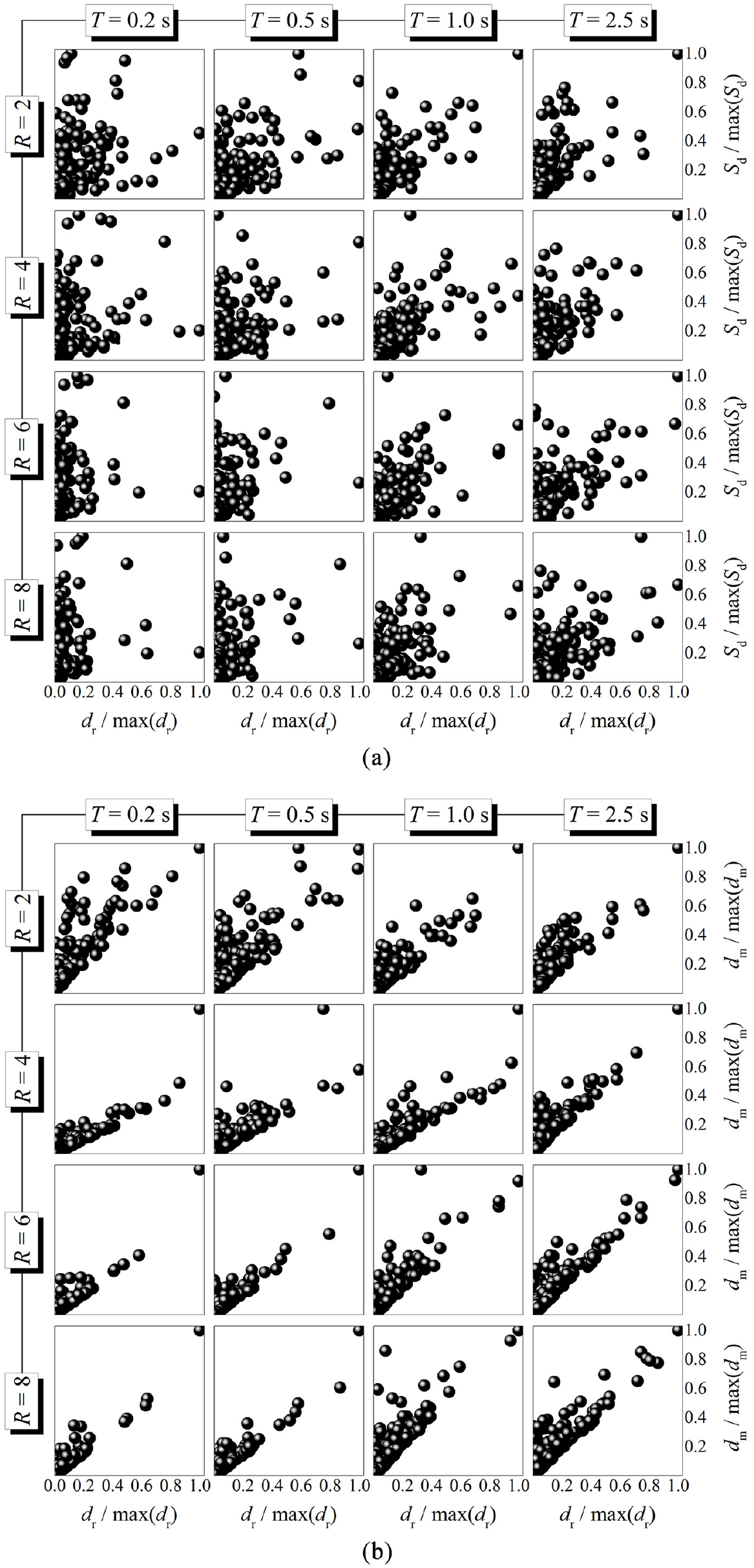
Scatter plots of residual displacements versus (a) elastic spectral displacements and (b) peak inelastic displacements.

To quantify this linear relationship, Pearson’s correlation coefficients ρ between the residual displacements and the intermediates (S_d or d_m) were computed as presented in Figure 7. It can be seen that, regardless of hysteretic rules, the residual displacements have a stronger correlation with the peak inelastic displacements than with the elastic spectral ones, particularly for short to intermediate period ranges (T < 1.0 s). In general, the linear correlation between the residual displacements and the peak inelastic displacements is not significantly influenced by T and R, and the averaged correlation coefficients neglecting the effect of T and R are roughly 0.89, 0.86, and 0.76, respectively, for elastoplastic, Thin Takeda, and Fat Takeda systems. In view of this stronger correlation, the peak inelastic displacement appears to be a better intermediate step for residual displacement demands estimation, since the residual displacement normalized by peak inelastic displacement is expected to exhibit lower dispersion. To confirm this, a comparison between two residual displacement ratios in terms of their dispersion is carried out next.

Figure 7.

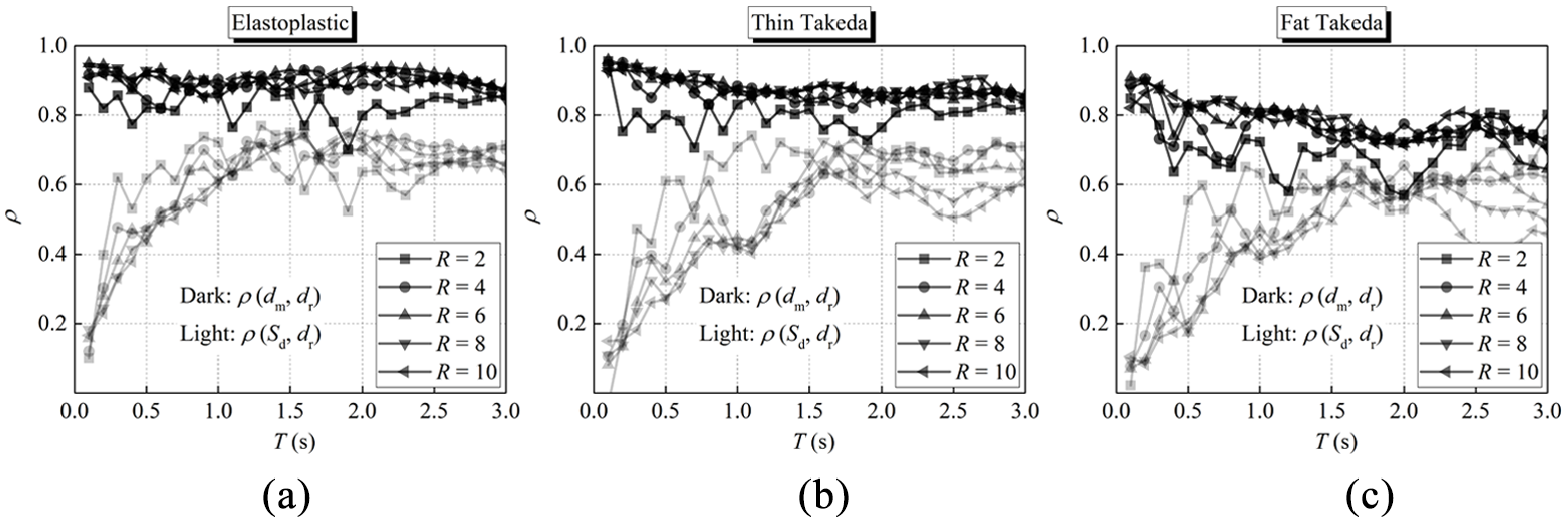
Correlation between residual displacements and elastic spectral displacements as well as peak inelastic displacements for (a) elastoplastic, (b) thin Takeda, and (c) fat Takeda systems.

Dispersion of residual displacement ratios

The dispersion of residual displacement ratios was quantified by computing their COV. Figure 8 presents the COV of residual displacement ratios, C_e and C_p, for elastoplastic, Thin Takeda, and Fat Takeda hysteretic SDOF systems under 240 ground motions.

Figure 8.

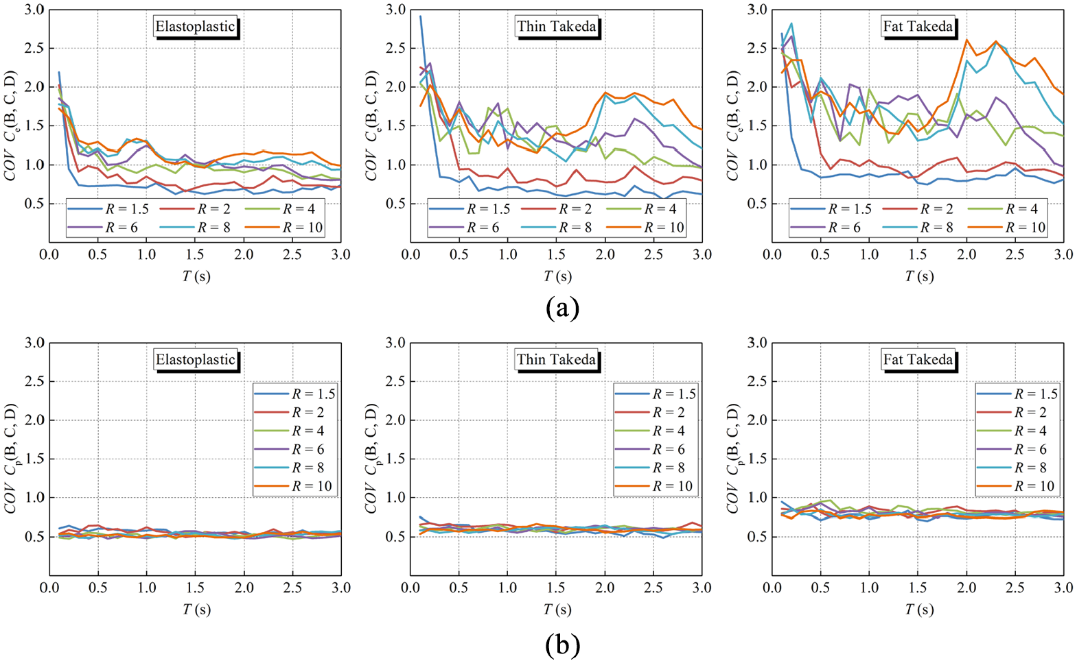
Coefficients of variation of (a) C_e and (b) C_p computed from all 240 ground motions.

By comparing Figure 8a and b, it can be observed that the COV of C_e and C_p shows different tendencies in statistical sense. In general, dispersion of C_e tends to increase as the relative lateral strength increases. For very short period ranges (T < 0.3 s), dispersion of C_e is especially high regardless of relative lateral strength. However, dispersion of C_p is almost independent of T and R, and the averaged COV of C_p neglecting the effects of T and R is about 0.53, 0.60, and 0.80 for elastoplastic, Thin Takeda, and Fat Takeda hysteretic systems. It is thus concluded that for a given T and R, the estimation of C_e involves larger uncertainty than the estimation of C_p. This is particularly true for high levels of relative lateral strength or for very short period ranges. For instance, for R > 4, the COV of C_e is more than twice the COV of C_p, and is, on average, nearly triple for T < 0.3 s.

To provide a visual representation about the variation, or spread of samples, Figure 9 shows the vertically aligned boxplots of C_e (in red) and C_p (in blue) for elastoplastic systems with combinations of R = 2, 4, and 6 and T = 0.3, 1.0, and 2.5 s. Details of a typical boxplot are illustrated in the first subplot, and its implementation is available in Montgomery and Runger (2014). It can be observed that the distribution of C_e is highly right-skewed with a considerable number of outliers, especially for short period ranges and for high levels of relative lateral strength. Nevertheless, the distribution of C_p seems to be fairly symmetric without any outliers. Note that the C_p does not follow a strictly symmetric distribution. Actually, the Kolmogorov–Smirnov (K-S) test suggests that the C_p can be reasonably characterized by a beta distribution bounded between 0 and 1, and the C_e follows a lognormal distribution, which is consistent with those in Liossatou and Fardis (2015).

Figure 9.

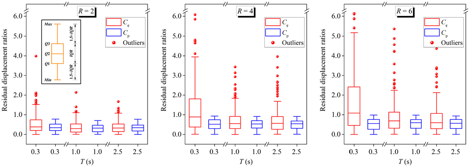
Boxplots for residual displacement ratios computed for elastoplastic systems.

Typically, the response spectrum has been recognized as a conventional approach for the estimation of residual displacement demands. However, such a response spectrum, constructed based on the statistical average of a large number of NTHA results, is particularly susceptible to the outliers, and is not an appropriate representative of the samples with large dispersion or with skewed distribution as well. As previously mentioned, the residual-to-peak-inelastic displacement ratios C_p have the advantages of small dispersion, fairly symmetric distribution, and samples without any outliers, which make C_p more appropriate for construction of the average residual displacement spectrum. This affirmation, however, is based on the premise that the d_m is predicted with reasonable accuracy. Conversely, if d_m is estimated with a higher uncertainty than S_d, the residual displacement ratio C_p may no longer be a preferable option.

With the objective of making a comparison between two methodologies in terms of the convenience of engineering application and thus developing reasonable response spectra, the following sections focus on the dependence of residual displacement ratios on ground motion and structural characteristics.

Effects of ground motion and structural characteristics

Effect of local site conditions

As is known to all, the local site conditions have a profound effect on the elastic response spectra (as illustrated in Figure 2). This effect is generally considered by specifying different shapes of spectra in the current seismic specifications or standards, such as ASCE 7-10 (American Society of Civil Engineers (ASCE), 2013), FEMA-450 (FEMA, 2003), and GB 50011-2010 (National Standard of the People’s Republic of China, 2010). There is, however, no consensus concerning the influence of site conditions on residual displacement demands. For instance, Kawashima et al. (1998) concluded that the residual displacements are almost independent of soil conditions. On the contrary, Ruiz-García and Miranda (2006b) suggested that such effect is large and need to be considered while estimating residual displacement demands. Therefore, a further look at the effect of local site conditions on residual displacement demands is pertinent.

Mean residual displacement ratios for different firm sites

The residual displacement ratios, C_e and C_p, corresponding to the three groups of local site conditions considered herein were computed for SDOF systems using TSPD model. Figure 10 presents the mean residual displacement ratios for elastoplastic and Thin Takeda systems. The results of Fat Takeda systems are not given, since they show a similar trend with those of Thin Takeda. As can be seen, the influence of site conditions on C_e is significantly larger than that on C_p, which is mainly embodied in two aspects.

Figure 10.

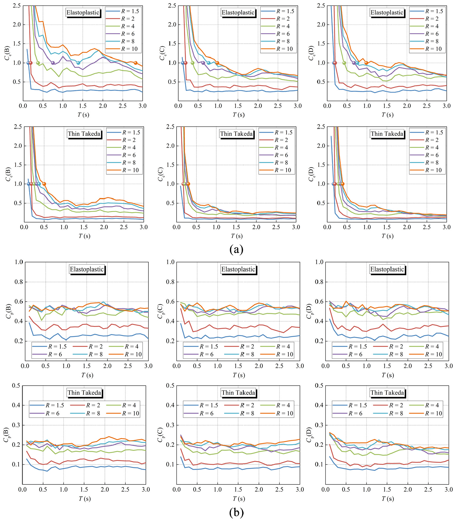
Mean residual displacement ratios (a) C_e and (b) C_p corresponding to site classes B, C, and D.

On the one hand, the limiting period, where the residual displacement exactly equals to the elastic spectral one (i.e. C_e = 1), is longer for rock sites than for soft sites, which is particularly true for high levels of R or for non-degrading hysteretic systems. For instance, for elastoplastic systems with R = 10, site class B corresponds to a limiting period of about 2.82 s, while site class C (or D) corresponds to a limiting period of merely about 0.98 s.

On the other hand, to quantify the effect of local site conditions, the mean residual displacement ratios computed from each site class are normalized by the mean residual displacement ratios computed from all 240 ground motions, and the obtained normalized residual displacement ratios are presented in Figure 11. As can be inferred, the normalized residual displacement ratio less than one implies that for a certain site class neglecting the effect of site conditions will lead to an overestimation of residual displacement demands. However, the normalized residual displacement ratio greater than one means an underestimation. Exactly, the normalized residual displacement ratio equal or very close to one indicates that the effect of site conditions may be negligible. Moreover, the greater the extent to which normalized residual displacement ratios deviate from one, the larger the errors produced by neglecting the effect of site conditions.

Figure 11.

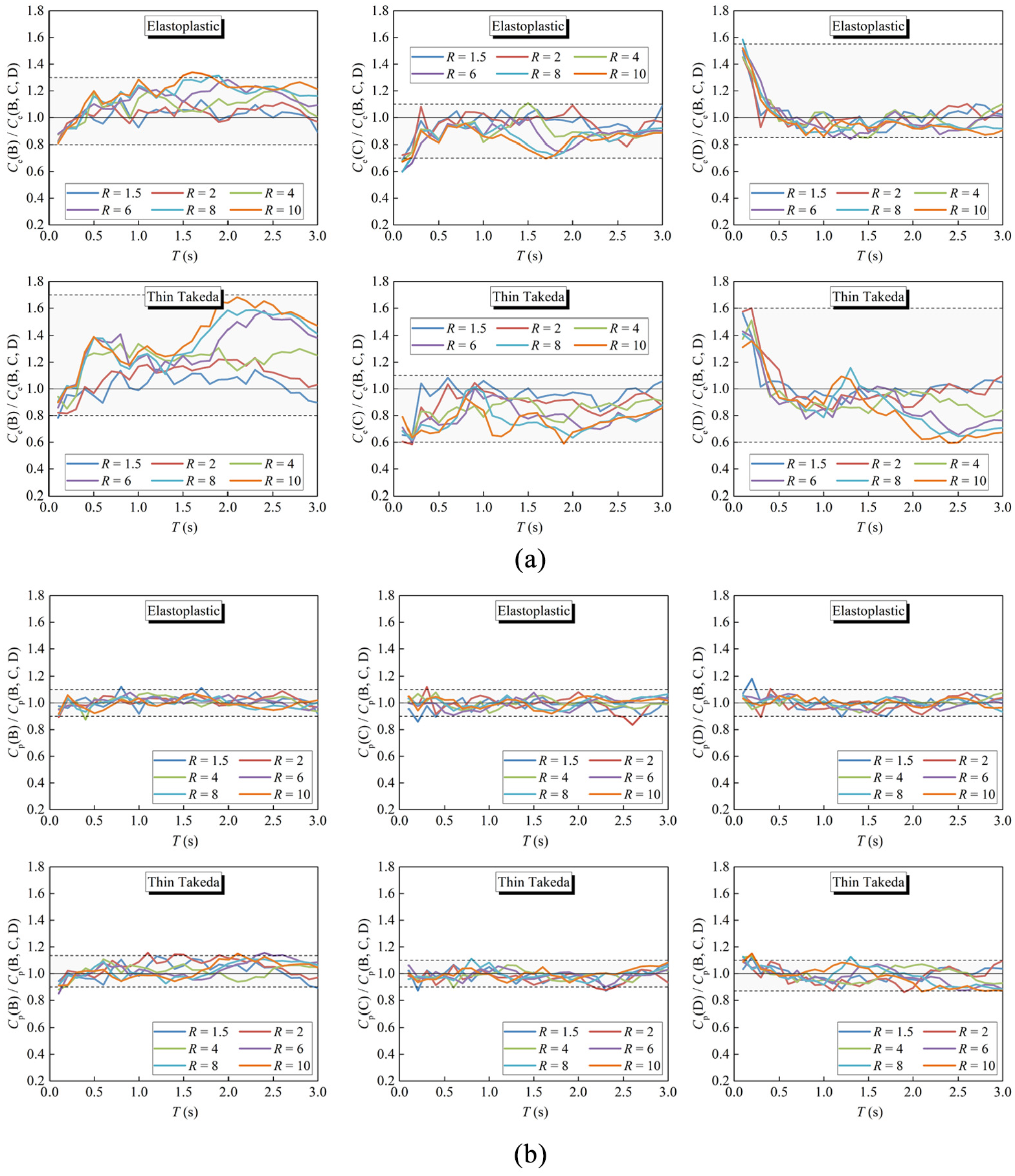
Mean residual displacement ratios (a) C_e and (b) C_p computed from each site condition normalized by mean residual ratios computed from all 240 ground motions.

A comparison of Figure 11a and b shows that, in general, the use of C_e will introduce much greater errors than the use of C_p, provided that the residual displacement demands for a certain site condition (e.g. sites B, C, or D) are estimated directly by using the results from all 240 ground motions. This observation is particularly pronounced for structures with degrading hysteretic rules (e.g. Thin/Fat Takeda) or with weak strength. A typical case is that, for very high levels of relative lateral strength (R ≥ 6), the normalized C_e spectra for Takeda systems are locally amplified over the long period range, which, however, is not observed in elastoplastic systems. In general, neglecting the site effects would, on average, result in an underestimation of residual displacement ratios, C_e, up to about 23%, 45%, and 56%, respectively, for elastoplastic, Thin Takeda, and Fat Takeda systems with R = 10 and periods larger than 0.5 s constructed at site class B. However, for residual displacement ratios, C_p, the errors (underestimation or overestimation) produced by neglecting the effect of local site conditions are, in general, smaller than 10%, regardless of the natural periods, the levels of lateral strength, and the hysteretic rules.

For practical application situations, the effect of site conditions on the mean residual displacement ratios, C_p, is relatively small and can be neglected. This observation, however, does not necessarily apply to far-field long-duration earthquake ground motions with different frequency contents, and its validity requires further investigation.

Dispersion of residual displacement ratios for different firm sites

Figure 12 presents the COV of residual displacement ratios, C_e and C_p, corresponding to site classes B, C, and D. It can be seen that the COV of C_p is almost independent of the local site conditions over the whole period range considered, while the COV of C_e is largely affected by the site conditions. In particular, for short period ranges, the C_e ratios corresponding to site class C exhibit larger dispersion. For longer period ranges, the C_e ratios corresponding to site class B tend to produce larger dispersion.

Figure 12.

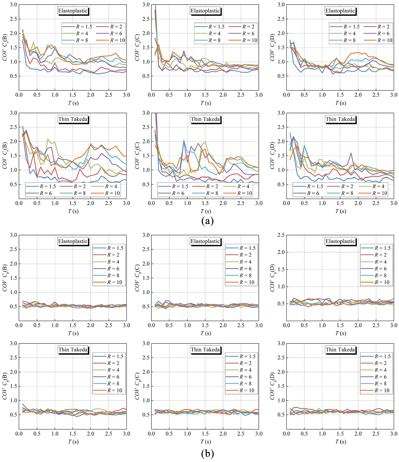
Coefficients of variation of (a) C_e and (b) C_p for systems corresponding to site classes B, C, and D.

Residual displacements, peak inelastic displacements, and elastic spectral displacements for different firm sites

From the above analysis, the effect of local site conditions is largely dependent on which intermediate is used for normalizing the residual displacement demands. To understand this dependence, a brief look at the effect of site conditions on residual displacements and on each intermediate (S_d or d_m) may be helpful. To this end, the residual displacement (d_r), peak inelastic displacement (d_m), and elastic spectral displacement (S_d) are computed for each earthquake record, of which the ground acceleration is scaled in the same way as in Figure 2 (i.e. the PGA of each record is 1 m/s²). Figure 13 presents the counted median spectra of d_r, d_m, and S_d for elastoplastic systems, among which the first two spectra (d_r and d_m) correspond to the case of R = 6.

Figure 13.

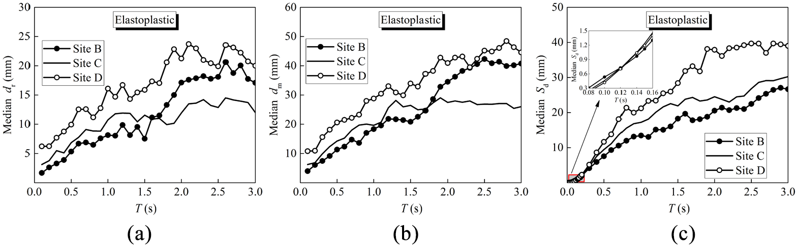
(a) Residual displacements, (b) peak inelastic displacements, and (c) elastic spectral displacements corresponding to site classes B, C, and D.

A comparison of Figure 13a and b shows that, the effect of local sites on d_m spectra is very similar to that on d_r spectra. For instance, for periods less than about 1.6 s, the structures on site class B tend to produce the smallest d_r and d_m, while for periods greater than about 1.6 s, the structures on site class C tend to produce the smallest d_r and d_m. Moreover, the structures located on site class D are prone to experience larger d_m as well as d_r than those on other sites (site classes B and C), regardless of natural periods. It appears that such similarity between d_m and d_r spectra would weaken the effect of site conditions on d_m normalized residual displacements (i.e. C_p) in terms of not only central tendencies but also dispersions, which provides a good explanation of how the effect of site conditions depends on the normalization of residual displacements.

Estimation of residual displacements for different firm sites

In general, when Equation 1 is employed, the absolute values of residual displacements can be determined by the multiplication of S_d to C_e, both of which, however, are significantly affected by local site conditions. Therefore, the local site influence should be, respectively, taken into account while determining S_d and C_e. The current seismic specifications or standards generally specify many site classifications. For instance, up to four firm site classifications have been specified in FEMA-450 (FEMA, 2003) and ASCE 7-10 (ASCE, 2013). As a result, the approach to estimate the residual displacements using Equation 1 has to repeatedly consider the influence of local site conditions, which results in a cumbersome work. Similarly, when Equation 2 is used, the absolute values of residual displacements can be determined by the multiplication of d_m to C_p, among which the C_p is almost independent of local site conditions. Consequently, only the effect of site conditions on d_m needs to be considered when the residual displacements are estimated by Equation 2. To sum up, for the convenience of engineering application, the C_p is superior to the C_e for residual displacements prediction.

Effect of ground motion duration

In this section, the effect of ground motion duration on residual displacement ratios is examined using the significant duration defined by Trifunac and Brady (1975). To isolate the influence of local site conditions, the ground motions used for analysis should be recorded in the same site. As an example, the records in site class C are considered as the database. According to the computed significant duration, these records are averagely divided into two subsets (each contains 40 records), respectively, having short duration (SD), ranging between 2.4 and 11.0 s, and long duration (LD), between 11.3 and 36.4 s. A comparison of mean C_e and C_p computed from each subset is presented in Figure 14 for three levels of relative lateral strength.

Figure 14.

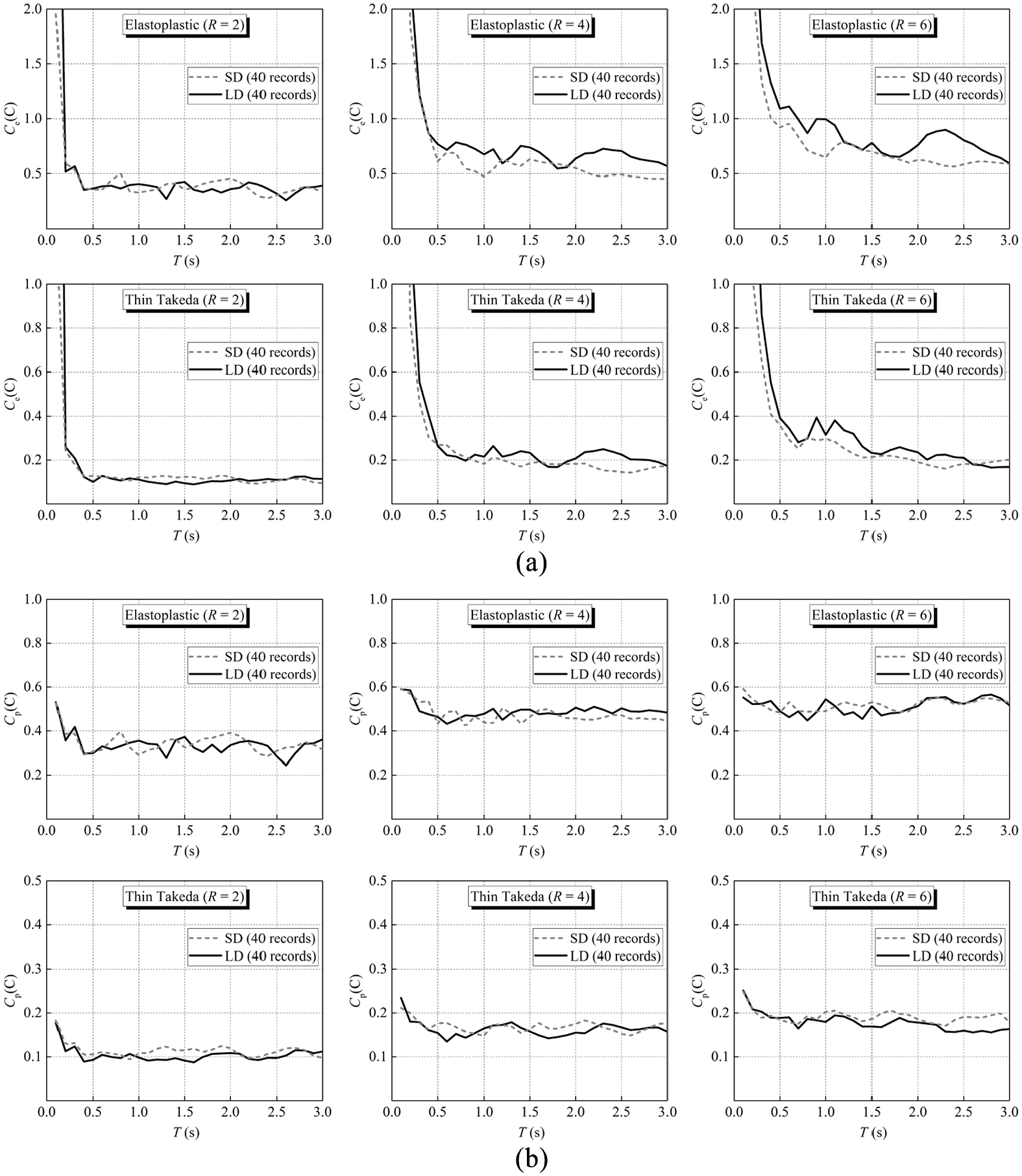
Effect of ground motion duration on mean residual displacement ratios (a) C_e and (b) C_p for three levels of relative lateral strength.

It can be seen that the influence of significant duration on C_e is larger than that on C_p. In general, the effect of significant duration on C_e depends on relative lateral strength. For low levels of relative lateral strength, ground motion duration has less effect on C_e, while for higher levels of relative lateral strength (i.e. R ≥ 4), LD ground motions will produce larger C_e ordinates than SD ground motions in the mean sense. This is consistent with the findings of Ruiz-García (2010). In addition, the effect of significant duration is larger for elastoplastic systems than for Takeda systems. For instance, for elastoplastic and Thin Takeda systems with R = 6, C_e ordinates computed from LD ground motions are on average 22% and 15% greater than those from SD ground motions, respectively. However, the mean C_p spectra computed from two sets of records (SD and LD) are fairly close to each other, regardless of relative lateral strength, and ground motion duration does not appear to have significant effect on C_p ratios.

Effect of structural characteristics

A statistical analysis is carried out to investigate the effect of structural characteristics, such as hysteretic rules, periods of vibration and relative lateral strength, on residual displacement ratios. For simplicity, the influence of ground motion characteristics is not included, and the following section focuses on residual displacement ratios computed for ground motions recorded on firm site conditions ( $v_{s, 30} \geq 180 m / s$ ).

Figure 15 shows the mean residual displacement ratios for elastoplastic, Thin Takeda, and Fat Takeda hysteretic SDOF systems subjected to all 240 ground motions. It can be seen that the residual displacement ratios computed for non-degrading (elastoplastic) and degrading (Thin/Fat Takeda) systems show similar trends, but with the significant difference in ordinates. In particular, for a given period of vibration and yield strength reduction factor, the elastoplastic systems always produce the largest residual displacement ratios, followed by the Thin Takeda systems and last the Fat Takeda systems. Note that these observations hold true both for C_e and C_p. However, the dependence of C_e on hysteretic rules indicates that residual displacements decrease from elastoplastic to Thin Takeda, and further to Fat Takeda, which does benefit from re-centering hysteretic characteristics. This observation is qualitatively in line with those in Christopoulos et al. (2003), Liossatou and Fardis (2015), and Ruiz-García and Miranda (2006b).

Figure 15.

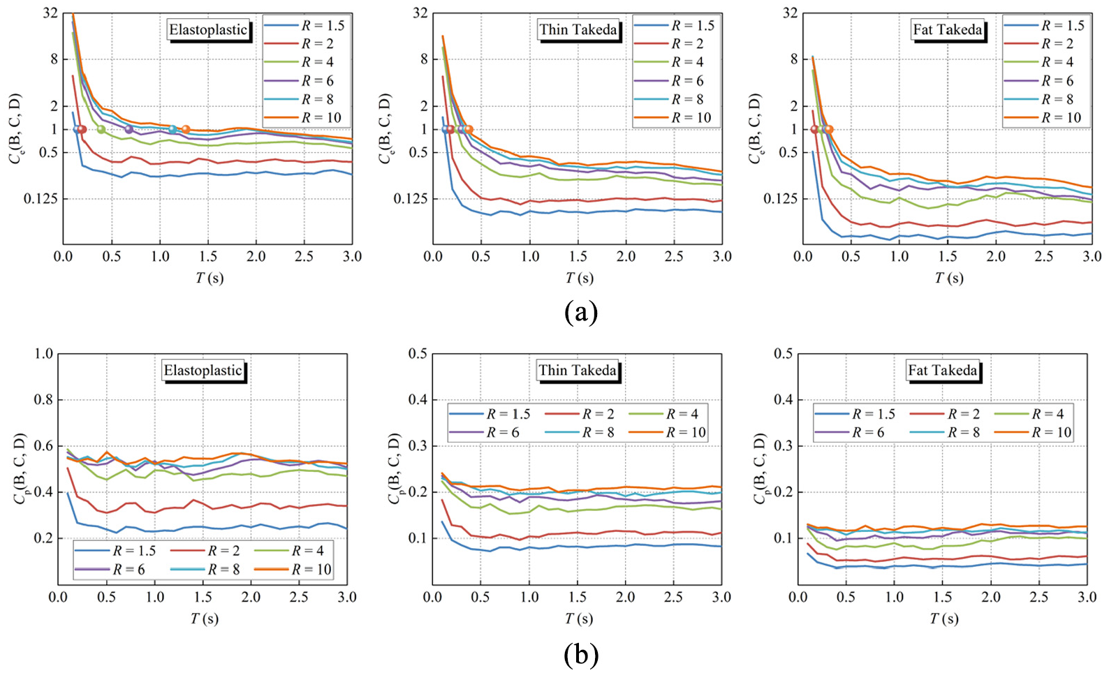
Mean residual displacement ratios (a) C_e and (b) C_p computed from all 240 records.

By comparing Figure 15a and b, it can be observed that the C_e and C_p spectra exhibit somewhat different tendencies in the mean sense. The first difference is related to the dependence of natural periods. In general, the mean C_e ordinates sharply increase as the natural periods decrease for T < 0.5 s, regardless of the relative lateral strength. For instance, for elastoplastic systems with R = 4, the mean C_e ordinate at T = 0.1 s is roughly 20 times that at T = 0.5 s. However, with the exception of strong structures with very short periods (i.e. R < 4 and T < 0.3 s), the C_p spectra are almost independent of natural periods.

Another difference between C_e and C_p spectra is associated with the dependence of relative lateral strength. To facilitate the discussion, Figure 16 depicts the mean residual displacement ratios, C_e and C_p, as a function of R for three different hysteretic models. As can be seen from Figure 16a, the longer the natural period, the slower the rate at which the mean C_e increases with the increase of R. In particular, for the long period structure (i.e. T ≥ 1.0 s), the mean C_e tends to saturate as the R increases. Note, however, that such observations do not always hold true for the mean C_p as shown in Figure 16b, where two spectral regions can be identified, regardless of natural periods and hysteretic rules. In the first region (R < 4), the mean C_p increases as the R increases. In the second region (R ≥ 4), the mean C_p is almost independent of R.

Figure 16.

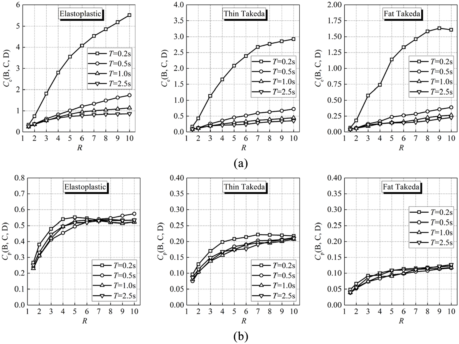
Effect of yield strength reduction factors on mean residual displacement ratios (a) C_e and (b) C_p.

Overall, the independence of residual displacement ratios C_p on T and on R beyond a value of about 4 makes C_p more convenient for engineering application. Moreover, this observation has important implications in seismic engineering. Recall that the statistical results indicate that the inelastic displacement ratios (defined as ratios of peak inelastic to elastic spectral displacements) are almost independent of T and R in certain spectral regions, which give rise to the well-known “equal displacement rule” (Veletsos and Newmark, 1960). By analogy, the residual displacement ratios C_p can relate the residual and peak inelastic displacements together without any influence of T and of R for R ≥ 4. Therefore, for medium to high values of R, the residual displacement follows the “(proportionally) equal residual displacement rule.” The similar rule has also been reported by Hatzigeorgiou et al. (2011).

Constant-strength residual displacement spectra

The C_p methodology is preferred over the C_e for the residual displacement demands estimation in terms of not only accuracy but also convenience of engineering application, provided that the peak inelastic displacement is estimated with a low uncertainty. However, if the peak inelastic displacements are indirectly estimated from elastic spectral ones (i.e. via inelastic displacement ratios) that are known a prior, additional uncertainty due to this intermediate step could be introduced. Particularly, if such uncertainty in the estimation of the peak inelastic displacements is far larger than that of the elastic spectral displacements, then the residual displacement ratios C_p may no longer be a preferred option. For providing alternatives to estimate the residual displacement demands, both two normalizations (C_e and C_p) are considered in this study for development of the average residual displacement spectra.

According to the statistical results, the following uniform functional forms, which can reasonably describe the dependence of the estimated parameters on various independent variables, are respectively proposed to predict the mean residual displacement ratios, C_e and C_p, for the three typical hysteretic systems. Note that the proposed equations for both two types of normalizations satisfy the fundamental condition of $C_{e} (R = 1) = 0$ and $C_{p} (R = 1) = 0$ , which, evidently, results from the fact that the structures behaving elastically do not sustain any permanent deformations. In addition, the influence of significant duration is not included in the mean C_e spectra because of the insufficient dataset.

C_{e} = (R - 1) [\frac{aR}{T^{b} \exp (T)} + \frac{c}{R^{d}}]

(4)

and

C_{p} = \frac{R - 1}{aR + b}

(5)

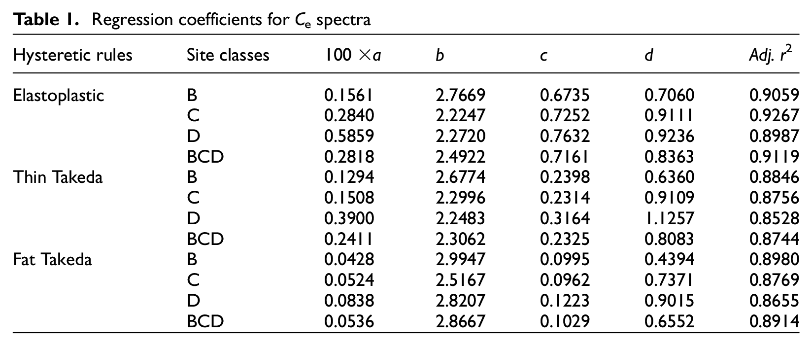
where a, b, c, and d in Equation 4 are the constants depending on the local site conditions and hysteretic rules, and the constants a and b in Equation 5 only depend on hysteretic rules. The values of these constants can be determined by the nonlinear regression analysis using the Levenberg–Marquardt iteration algorithm. The final determined regression coefficients for both two residual displacement spectra are summarized in Tables 1 and 2, where the adjusted determination coefficients (Adj. r²) are also provided.

Table 1.

Regression coefficients for C_e spectra

Hysteretic rules	Site classes	100 ×a	b	c	d	Adj. r ²
Elastoplastic	B	0.1561	2.7669	0.6735	0.7060	0.9059
	C	0.2840	2.2247	0.7252	0.9111	0.9267
	D	0.5859	2.2720	0.7632	0.9236	0.8987
	BCD	0.2818	2.4922	0.7161	0.8363	0.9119
Thin Takeda	B	0.1294	2.6774	0.2398	0.6360	0.8846
	C	0.1508	2.2996	0.2314	0.9109	0.8756
	D	0.3900	2.2483	0.3164	1.1257	0.8528
	BCD	0.2411	2.3062	0.2325	0.8083	0.8744
Fat Takeda	B	0.0428	2.9947	0.0995	0.4394	0.8980
	C	0.0524	2.5167	0.0962	0.7371	0.8769
	D	0.0838	2.8207	0.1223	0.9015	0.8655
	BCD	0.0536	2.8667	0.1029	0.6552	0.8914

Table 2.

Regression coefficients for C_p spectra

Hysteretic rules	a	b	Adj. r ²
Elastoplastic	1.7074	−0.5560	0.9389
Thin Takeda	4.3687	0.0284	0.9175
Fat Takeda	7.1313	3.2500	0.9306

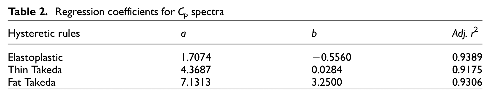
A comparison of statistical mean residual displacement ratios with those computed using the proposed equations is presented in Figures 17 and 18, respectively, for C_e and C_p spectra. The figures and the Adj. r² values all demonstrate that the proposed response spectra provide reasonably accurate estimates of mean residual displacement ratios.

Figure 17.

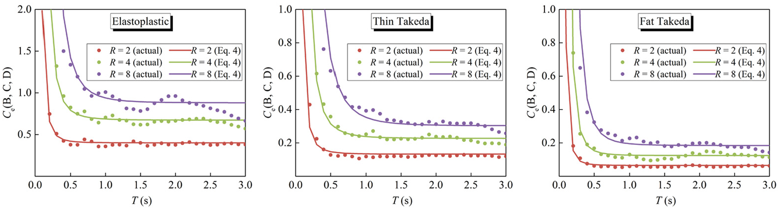
Comparison of actual (NTHA results) and estimated C_e for three typical hysteretic systems.

Figure 18.

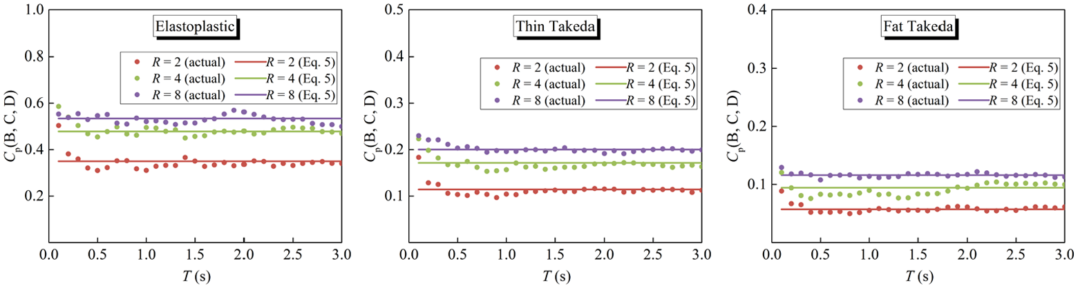
Comparison of actual (NTHA results) and estimated C_p for three typical hysteretic systems.

It is interesting to note that Ruiz-García and Miranda (2006b) proposed the mean C_e spectrum to estimate the residual displacement demands. This spectrum, however, is based on statistical results of the nonlinear dynamic analysis using ISPD assumption. Hence, with the objective of having a look at the effect of viscous damping models on residual displacement demands, a comparison of their results with those developed in this work may be helpful.

Figure 19 shows a comparison of mean C_e spectra from Ruiz-García and Miranda (2006b) with those from Equation 4 for elastoplastic systems with R = 4. It can be observed that the C_e ordinates computed from Equation 4 are larger than those from Ruiz-García and Miranda (2006b) over the whole period range considered, indicating that the TSPD will lead to larger residual displacement ratios C_e and, in consequence, in larger residual displacement demands than the ISPD. Note that Priestley and Grant (2005) obtained the similar findings in investigating the influence of damping models on peak inelastic displacements. Regarding the effect of initial viscous damping models on residual displacement demands, a comprehensive study has been carried out by Feng and Gong (2020), and further details are available in that study.

Figure 19.

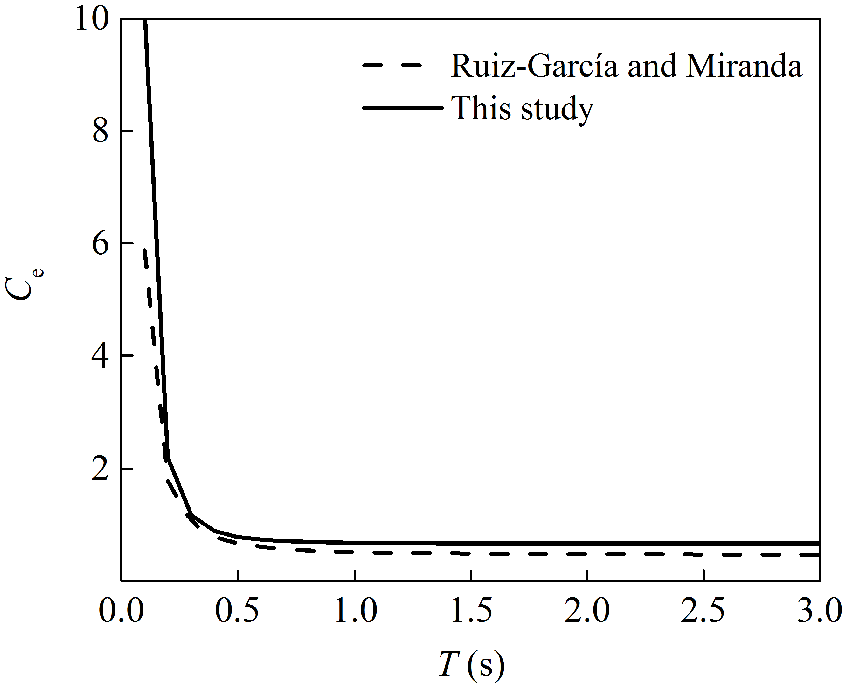
Comparison of mean C_e spectra from Ruiz–García and Miranda with those from Equation 4 for R = 4.

Discussion on extension to MDOF systems

Although this study clarifies the applicability of various normalizations and develops simple expressions, it is still restricted to the structures that can be simplified to SDOF systems. For more complex multi-degree-of-freedom (MDOF) structures, the residual displacement demands or residual story drift demands largely depend on additional factors (Christopoulos and Pampanin, 2004; Pampanin et al., 2003; Ruiz-García and Miranda, 2006a), among which the following are expected to matter more:

(1) P-Δ effects

For generic frame structures exhibiting relatively high levels of inelastic behavior, the maximum story drift demands are found to be concentrated at the bottom stories (Medina and Krawinkler, 2003). As a consequence, the structural P-Δ effects may become of particular importance to these lower stories, which can reduce the post-yield stiffness to a pretty small or even negative value, thus resulting in a large residual drift being unrecoverable.

(2) Failure mechanism

The frame structures are generally designed according to the strong-column and weak-beam philosophy. In this way, the structures are expected to adhere to an ideal beam-hinge mechanism, which would be beneficial to avoid damage on the columns or damage concentration. As a result, the beam-hinge frames are more prone to recover from inelastic excursion than frames developing other undesirable failure types such as column-hinge and full-hinge mechanisms. More specifically, it seems that the beam-hinge mechanism would exhibit the re-centring hysteretic characteristics that restrain the permanent deformations (Ruiz-García and Miranda, 2006a).

(3) Higher modes

As previously mentioned, the beam-hinge frames are expected to yield more uniform distribution of story drift along the height, whereas the column-hinge frames lead to a story drift concentration at lower stories (Medina and Krawinkler, 2003). Hence, it can be inferred that the frames developing column-hinge mechanism would be more influenced by higher modes than those with beam-hinge mechanism.

The aforementioned aspects may largely restrict the application of the observations and relations to more complex MDOF systems. However, these aspects can be approximately considered by using the amplification factors, which is analogy to those adopted for the evaluation of maximum displacement/drift demands (Gupta and Krawinkler, 2000). By this way, the proposed equations for SDOF systems can be extended to the estimation of residual drift demands of MDOF frame structures. The development of amplification factors in MDOF structures is the subject for further investigation and the results will be available in the future.

Conclusion

A comprehensive study is implemented to clarify the pros and cons of each normalization format for the estimation of residual displacements. The residual-to-peak-inelastic displacement ratios are preferred over the residual-to-elastic-spectral displacement ratios for the following reasons, provided that the peak inelastic displacement is estimated with a low uncertainty:

The residual displacements have a stronger linear correlation with the peak inelastic displacements than with the elastic spectral ones, especially for short to medium period structures (T ≤ 1.0 s).

The residual-to-peak-inelastic displacement ratios have the advantages of small dispersion, samples without any outliers and relatively symmetric distribution, which make the residual-to-peak-inelastic displacement ratios more appropriate for development of the average residual displacement spectrum.

The residual-to-peak-inelastic displacement ratios are almost independent of the local site conditions, natural periods, significant duration, and yield strength reduction factors beyond a value of about 4, which is convenient for engineering application.

The residual-to-peak-inelastic displacement ratios that allow the estimation of residual displacement demands from peak inelastic displacement demands emphasize that the post-earthquake reparability assessment should be based on the premise of no collapse, which consequently matches well with the current seismic performance assessment procedures.

However, if the peak inelastic displacement is estimated with a much higher uncertainty than the elastic spectral displacement, then the residual-to-peak-inelastic displacement ratios may no longer be a preferred option. Finally, the residual displacement spectra, which allow the estimation of residual displacements in terms of both elastic spectra and peak inelastic displacements are developed for three typical hysteretic systems.

Footnotes

Authors’ note

Any opinions, findings, and conclusions or recommendations expressed in the study are those of the authors and do not necessarily reflect the views of the National Natural Science Foundation of China.

Declaration of conflicting interests

The author(s) declared no potential conflicts of interest with respect to the research, authorship, and/or publication of this article.

Funding

The author(s) disclosed receipt of the following financial support for the research, authorship, and/or publication of this article: The authors acknowledge the financial support from the National Natural Science Foundation of China under Grant Nos 51678104 and 51978125.

ORCID iD

Zhibin Feng

References

Ali

Khan

Ashraf

Ahmed

(2013) Seismic performance of stone masonry buildings used in the Himalayan Belt. Earthquake Spectra 29(4): 1159–1181.

American Society of Civil Engineers (ASCE) (2013) Minimum Design Loads for Buildings and Other Structures, ASCE/SEI 7-10. Reston, VA: ASCE.

Amiri

Bojórquez

(2019) Residual displacement ratios of structures under mainshock-aftershock sequences. Soil Dynamics & Earthquake Engineering 121: 179–193.

Borzi

Calvi

Elnashai

Faccioli

Bommer

(2001) Inelastic spectra for displacement-based seismic design. Soil Dynamics & Earthquake Engineering 21(1): 47–61.

Charney

(2008) Unintended consequences of modeling damping in structures. Journal of Structural Engineering 134(4): 581–592.

Chopra

McKenna

(2016) Modeling viscous damping in nonlinear response history analysis of buildings for earthquake excitation. Earthquake Engineering & Structural Dynamics 45(2): 193–211.

Christopoulos

Pampanin

(2004) Towards Performance-based seismic design of MDOF structures with explicit consideration of residual deformations. ISET Journal of Earthquake Technology 41(1): 53–73.

Christopoulos

Pampanin

Priestley

MJN

(2003) Performance-based seismic response of frame structures including residual deformations. Part I: Single-degree of freedom systems. Journal of Earthquake Engineering 7(1): 97–118.

Dazio

(2004) Residual displacements in capacity designed reinforced concrete structures, Paper No. 2399. In: Proceedings 13th world conference on earthquake engineering, Vancouver, BC, Canada, 1–6 August.

10.

Eguchi

Goltz

Taylor

Chang

Flores

Johnson

Seligson

Blais

(1998) Direct economic losses in the Northridge earthquake: A three-year post-event perspective. Earthquake Spectra 14(2): 245–264.

11.

Federal Emergency Management Agency (FEMA) (2003) NEHRP Recommended Provisions for Seismic Regulations for New Buildings and Other Structures—Part 1: Provisions, Tech. Rep. FEMA-450. Washington, DC: FEMA.

12.

Feng

Gong

(2020) Investigation on residual displacements for SDOF systems with various initial viscous damping models. Structures 28: 1831–1844.

13.

Fujino

Hashimoto

Abe

(2005) Damage analysis of Hanshin Expressway viaducts during 1995 Kobe earthquake. I: Residual inclination of reinforced concrete piers. Journal of Bridge Engineering 10(1): 45–53.

14.

Girija

Gupta

(2020) Scaling of constant-ductility residual displacement spectrum. Earthquake Engineering & Structural Dynamics 49: 215–233.

15.

Guerrero

Ruiz-García

(2017) Residual displacement demands of conventional and dual oscillators subjected to earthquake ground motions characteristic of the soft soils of Mexico City. Soil Dynamics & Earthquake Engineering 98: 206–221.

16.

Gupta

Krawinkler

(2000) Estimation of seismic drift demands for frame structures. Earthquake Engineering & Structural Dynamics 29(9): 1287–1305.

17.

Hall

(2006) Problems encountered from the use (or misuse) of Rayleigh damping. Earthquake Engineering & Structural Dynamics 35(5): 525–545.

18.

Hall

(2017) Discussion on “an investigation into the effects of damping and nonlinear geometry models in earthquake analysis” by Andrew Hardyniec and Finley Charney. Earthquake Engineering & Structural Dynamics 46(2): 341–342.

19.

Hardyniec

Charney

(2015) An investigation into the effects of damping and nonlinear geometry models in earthquake engineering analysis. Earthquake Engineering & Structural Dynamics 44(15): 2695–2715.

20.

Hardyniec

Charney

(2017) Response to Professor John Hall’s discussion of Hardyniec and Charney’s paper, “An investigation into the effects of damping and nonlinear geometry models in earthquake engineering analysis.” Earthquake Engineering & Structural Dynamics 46(2): 343–346.

21.

Hatzigeorgiou

Papagiannopoulos

Beskos

(2011) Evaluation of maximum seismic displacements of SDOF systems from their residual deformation. Engineering Structures 33(12): 3422–3431.

22.

Japan Road Association (JRA) (2002) Design Specifications of Highway Bridges. Part V: Seismic Design. Tokyo, Japan: JRA.

23.

Jehel

Léger

Ibrahimbegovic

(2014) Initial versus tangent stiffness-based Rayleigh damping in inelastic time history seismic analyses. Earthquake Engineering & Structural Dynamics 43(3): 467–484.

24.

Wen

Zhai

Katsanos

(2018) Residual displacement ratios of SDOF systems subjected to ground motions recorded on soft soils. Soil Dynamics & Earthquake Engineering 115: 331–335.

25.

Kanaan

Powell

(1973) A General Purpose Computer Program for Dynamic Analysis of Inelastic Plane Structures, Tech. Rep. DRAIN-2D. Berkeley, CA: Earthquake Engineering Research Center, University of California.

26.

Kawashima

MacRae

Hoshikuma

Nagaya

(1998) Residual displacement response spectrum. Journal of Structural Engineering 124(5): 523–530.

27.

Liossatou

Fardis

(2015) Residual displacements of RC structures as SDOF systems. Earthquake Engineering & Structural Dynamics 44(5): 713–734.

28.

Liossatou

Fardis

(2016) Near-fault effects on residual displacements of RC structures. Earthquake Engineering & Structural Dynamics 45(9): 1391–1409.

29.

MacRae

Kawashima

(1997) Post-earthquake residual displacements of bilinear oscillators. Earthquake Engineering & Structural Dynamics 26(7): 701–716.

30.

Mahin

Bertero

(1981) An evaluation of inelastic seismic design spectra. Journal of Structural Division 107(9): 1777–1795.

31.

Medina

Krawinkler

(2003) Seismic demands for nondeteriorating frame structures and their dependence on ground motions. Report No. 144. Stanford, CA: John A. Blume Earthquake Engineering Center.

32.

Montgomery

Runger

(2014) Applied Statistics and Probability for Engineers. 6th ed. Hoboken, NJ: John Wiley & Sons, Inc.

33.

National Standard of the People’s Republic of China (2010) GB 50011-2010: Code for Seismic Design of Buildings. Beijing, China: China Architecture and Building Press.

34.

Otani

(1974) SAKE: A computer program for inelastic response of R/C frames to earthquakes. Report UILU-ENG-74-2029. Urbana, IL: University of Illinois at Urbana-Champaign.

35.

Otani

(1980) Nonlinear dynamic analysis of reinforced concrete building structures. Canadian Journal of Civil Engineering 7(2): 333–344.

36.

Pacific Earthquake Engineering Research Center (PEER) (2019) PEER Strong Ground Motion Database. Available at: https://peer.berkeley.edu/peer-strong-ground-motion-databases (accessed 9 September 2019).

37.

Pampanin

Christopoulos

Priestley

MJN

(2003) Performance-based seismic response of frame structures including residual deformations. Part II: Multi-degree of freedom systems. Journal of Earthquake Engineering 7(1): 119–147.

38.

Paterson

Wang

(2008) The 2008 Wenchuan Earthquake: Risk Management Lessons and Implications. Beijing, China: Risk Management Solutions.

39.

Petrini

Maggi

Priestley

MJN

Calvi

(2008) Experimental verification of viscous damping modeling for inelastic time history analyzes. Journal of Earthquake Engineering 12(S1): 125–145.

40.

Priestley

MJN

Grant

(2005) Viscous damping in seismic design and analysis. Journal of Earthquake Engineering 9(spec. 02): 229–255.

41.

Priestley

MJN

Calvi

Kowalsky

(2007) Displacement-based Seismic Design of Structures. Pavia: IUSS Press.

42.

Quinde

Terán-Gilmore

Reinoso

(2020) Residual displacement estimation for soft soils: Application to Mexico city lake-bed. Soil Dynamics & Earthquake Engineering 130: 105970.

43.

Ramirez

Miranda

(2012) Significance of residual drifts in building earthquake loss estimation. Earthquake Engineering & Structural Dynamics 41(11): 1477–1493.

44.

Ruiz-García

(2010) On the influence of strong-ground motion duration on residual displacement demands. Earthquakes & Structures 1(4): 327–344.

45.

Ruiz-García

Guerrero

(2017) Estimation of residual displacement ratios for simple structures built on soft-soil sites. Soil Dynamics & Earthquake Engineering 100: 555–558.

46.

Ruiz-García

Miranda

(2006a) Evaluation of residual drift demands in regular multi-storey frames for performance-based seismic assessment. Earthquake Engineering & Structural Dynamics 35(13): 1609–1629.

47.

Ruiz-García

Miranda

(2006b) Residual displacement ratios for assessment of existing structures. Earthquake Engineering & Structural Dynamics 35(3): 315–336.

48.

Smyrou

Priestley

MJN

Carr

(2011) Modelling of elastic damping in nonlinear time-history analyses of cantilever RC walls. Bulletin of Earthquake Engineering 9(5): 1559–1578.

49.

Trifunac

Brady

(1975) A study on the duration of strong earthquake ground motion. Bulletin of the Seismological Society of America 65(3): 581–626.

50.

Veletsos

Newmark

(1960) Effect of inelastic behavior on the response of simple systems to earthquake motions. In: Proceedings 2nd world conference on earthquake engineering, vol. 2, pp. 895–912, Tokyo, Japan, 11–18 July.