Dataset from the shake table tests of a rocking podium structure

Abstract

Conventional validation of analytical and numerical models in Earthquake Engineering involves the comparison of numerically simulated response time histories to experimentally obtained benchmark responses to the same earthquake excitations. As the seismic design problem is inherently stochastic, an alternative, statistical, and easier-to-pass validation procedure has been suggested. As an example, numerical and analytical models may fail to predict the planar rocking response of a rigid block to a specific ground motion, but they can be proven quite successful in predicting the statistical distribution of the maxima of that response to an ensemble of ground motions. This article describes the publicly available data obtained from a series of 226 shake table tests of a 3D rocking podium structure, designed at ETH Zurich and carried out at EQUALS Lab, University of Bristol. This well-documented dataset is the largest one involving a shake table and can be used to statistically validate analytical and numerical models of rocking structures.

Keywords

Rocking wobbling shake table testing uplifting structures statistical model validation

Introduction

Rocking structures are the ones that can uplift from their base when subjected to an earthquake. The uplift works as a mechanical fuse limiting the design forces of both the superstructure and the foundation. This isolation property led researchers to propose rocking as a seismic design method for both buildings (Bachmann, 2018; Bachmann et al., 2017, 2019b; Cherepinskiy, 2004; Ríos-García and Benavent-Climent, 2020; Uzdin et al., 2009) and bridges (Agalianos et al., 2017; Dimitrakopoulos and Giouvanidis, 2015; Makris and Vassiliou, 2013, 2014; Vassiliou et al., 2017b). However, planar rocking is notoriously unpredictable by analytical or numerical models, while shake table tests of such systems have often proven to be non-repeatable (Bachmann et al., 2018; Anagnostopoulos et al., 2019 among others). Wobbling, a three-dimensional (3D) motion on a horizontal plane characterized by simultaneous uplift from the ground (rocking) and change of the contact point with the ground (nutation) without spinning or sliding out of its original position, like Euler’s disk (van den Engh et al., 2000; Vassiliou, 2018; Vassiliou et al., 2017a) is even harder to predict than planar rocking. Thus, developing seismic wobbling models is challenging, yet useful to further develop seismic design of realistic rocking structures expected to respond in all three dimensions, as well as to understand the seismic behavior of non-structural elements such as unanchored equipment (Bao and Konstantinidis, 2020; Dar et al., 2016, 2018; Di Egidio et al., 2015; Di Sarno et al., 2019; Konstantinidis and Makris, 2010; Sextos et al., 2017; Voyagaki et al., 2018; Wittich and Hutchinson, 2015).

Validation of wobbling models is a key step in this development process. Bachmann et al. (2018, 2019a) and Del Giudice et al. (2020) have suggested a statistical validation approach: they claimed that model validation in Earthquake Engineering should involve the prediction of the statistics of the response to an ensemble of ground motions (e.g. the cumulative distribution function of the maxima of the time history responses) rather than a prediction of the time history response to a specific excitation. This is a weaker (but still sufficient, given the probabilistic basis of seismic design acceptance criteria) validation procedure. It requires repeated shake table tests of an undamaged specimen under multiple earthquake excitations.

This data paper contains the results of multiple shake table tests of a 3D rocking podium structure, designed at ETH Zurich and built in Bristol. The tests were performed at the Earthquake and Large Structures Laboratory (EQUALS) of University of Bristol in the framework of the research project “Statistical verification and validation of 3D seismic rocking motion models (3DROCK),” which was selected for the Transnational Access part of the European Research Council Horizon 2020 project SERA. This article presents the conducted tests and the obtained dataset intended for statistical validation of numerical models of the seismic response of rocking and wobbling structures.

Specimen description

In order for the specimen to serve the purpose of the tests, it had to fulfill two criteria: (1) it should not accumulate damage (to enable statistical validation) and (2) it should be easy to reset after overturning as well as after a test that does not cause overturn. Therefore, the specimen shown in Figure 1 was designed. It comprises a slab supported on four wobbling circular columns resting on the shake table platform. The slab is made of 6082-T6 aluminum with a modulus of elasticity equal to 71 GPa. The total weight supported by the columns (i.e. of the aluminum slab and the restrainers) was computed equal to 605 kg, assuming steel and aluminum densities equal to 7850 and 2.7 kg/m³, respectively. The columns were made of S275 steel with a modulus of elasticity equal to 210 GPa. Their height, diameter, and wall thickness were 1000, 244.5, and 8 mm, respectively (Figure 2), giving them a slenderness ratio tan(α) = 0.2445. The size of the wobbling model is not representative of the size of a prototype bridge or a prototype podium building. Given that planar and 3D rocking response is size-dependent, the ground motion excitations used in the shake table experiments were scaled to preserve acceleration scaling (as discussed later in this data paper) so that the model represents a structure with a height similar to a real bridge.

Figure 1.

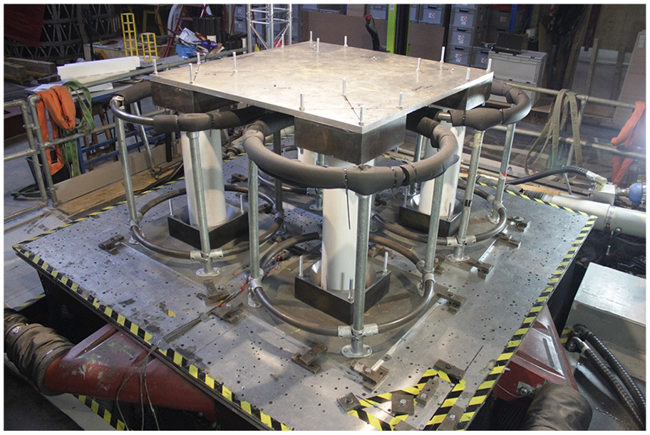
Wobbling specimen on the University of Bristol shake table.

Figure 2.

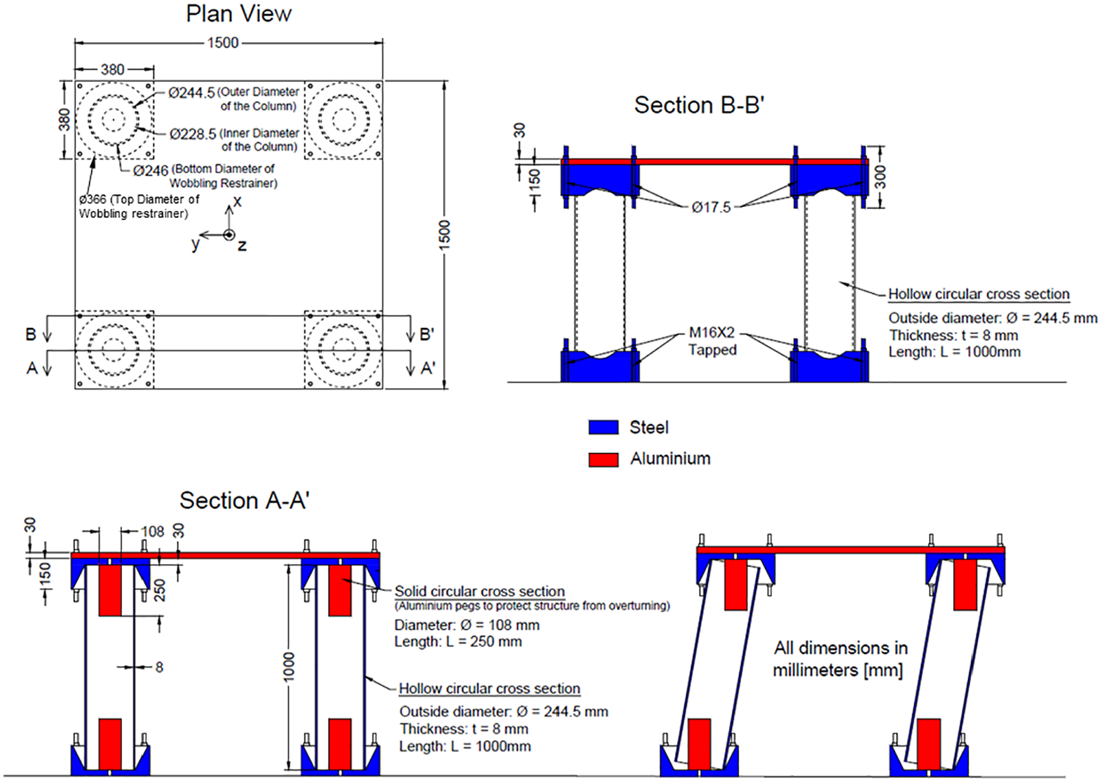
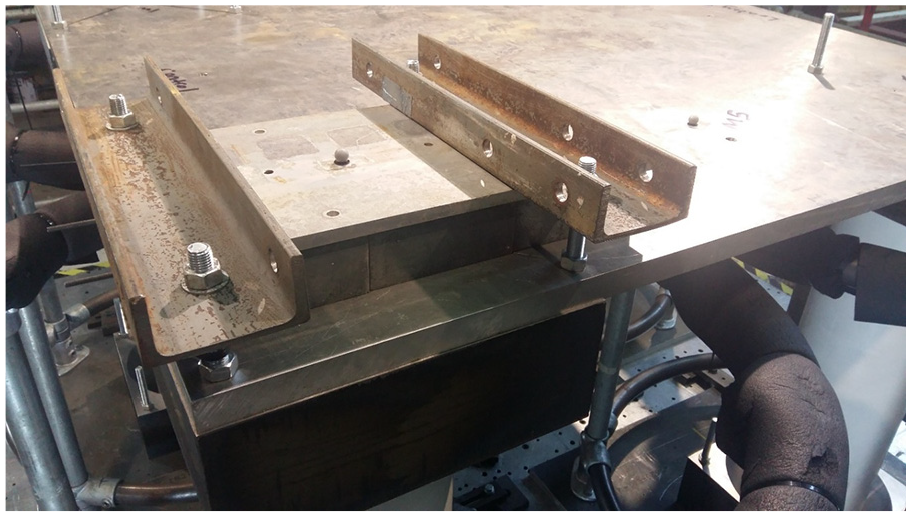
Details of the wobbling specimen.

The intention of wobbling model design was to mimic the assumptions of the “wobbling bridge” analytical model developed by Vassiliou et al. (2017a; Vassiliou, 2018), namely, that the structure is rigid and that the columns wobble without sliding or spinning about their longitudinal axis. To achieve this, the ends of the columns were machined (lathed) to ensure they are right angled to their longitudinal axis. Conical end-restrains were placed on each end of each column to stop the columns from wobbling out of their original position (Figure 3). Furthermore, aluminum pegs were installed inside the columns (Figure 3) with enough clearance to enable unrestrained wobbling up to overturning, and also engage early enough to enable easy recovery of the specimen to its original position after a test that resulted in overturning. Padded frames were placed under the specimen to protect the shake table platform (Figure 1).

Figure 3.

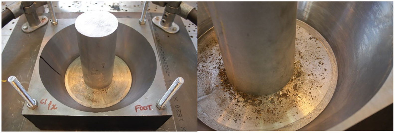
Conical restraint and an aluminum peg at the bottom of the wobbling specimen column before installation (left). Metal shavings found after the shake table tests show that the steel column scratched against the conical restrainer during the tests (right).

Specimen excitation using a shake table

The wobbling response of the specimen was induced by a dynamic bidirectional (two orthogonal horizontal components only) excitation of its base. This was achieved by placing the specimen on the top of the 6DOF 3 m × 3 m shake table of the University of Bristol (Shaking Table Specifications, n.d.). The stroke of the table is ±150 mm, and the maximum horizontal velocity is 1200 mm/s. The maximum acceleration of the table is 3.7 g and 1.6 g under 0 and 10,000 kg of payload, respectively.

Ground motions

There are several challenges related to ground motion selection and scaling that led us to use two particular recorded motions, namely, the 1940 El Centro and the 1999 Chi-Chi ground motion records. Two options were considered. One option was to select low-to-moderate amplitude ground motions based on the M-R pairs defined by the disaggregation of seismic hazard (to claim that the records were “site-specific”) and then scale them several times in amplitude to produce stronger motions. The problem with this option is that spectral matching is ill-defined, since the frequency range within which the mean spectrum needs to match the target one (e.g. (0.2 T₁to 1.5 T₁) in most seismic codes) depends on the fundamental period of the structure T₁, which, in the case of rocking and wobbling structures, evolves with ground motion intensity amplification and changes during the motion. The other option was to use a large sample of site-compatible (natural) records. Again, there is no specific T₁ for spectral matching or for procedure based on a conditional mean spectrum.

For the above reasons, the response spectra of two widely used (and scaled) recorded ground motions were used, and the motion-to-motion variability was introduced by generating compatible synthetic motions. The motions were synthesized using a spectral version of the Rezaeian and Der Kiureghian stochastic ground motion model (Broccardo and Dabaghi, 2017; Broccardo and Der Kiureghian, 2014; Rezaeian and Der Kiureghian, 2008). The generated synthetic motions are target-spectrum compatible − in other words, consistent with a given elastic acceleration response spectrum. A stochastic method to generate ground motions with similar power spectral density was adopted as the best-available precondition for a statistical comparison of the benchmark and model response datasets, even though motions with similar elastic spectra could have very different overturning potential (Bachmann et al., 2018). This is because the objective of this work is not to account for the full record-to-record ground motion variability at a given site, but to limit the analysis to ground motions that have a degree of spectral consistency (by matching the power spectral density) while retaining their stochastic properties in terms of amplitude and phase (given the target frequency content and the fixed pulse duration).

Note that such an approach serves the purpose of the conducted tests, that is, to explore the ability of numerical models to predict the mechanics of the prototype and at the same time to avoid complicated ground motion selection processes for a rocking system whose dynamic characteristics evolve in time.

Along these lines, two recorded ground motions, the 1940 El Centro Array #9 record and the 1999 Chi-Chi CHY080 record, were used as the “seed” ground motions for the experimental campaign (Figure 4a, b, g, and h). Next, two bidirectional (two orthogonal horizontal components) ground motion ensembles, each comprising 100 synthetic ground motions, were generated from the two seed ground motions. These two ground motion ensembles were used to drive the shake table during the tests after appropriate “training” of the table. Vertical ground motion and the three rotational excitations along the horizontal and vertical axes were not considered.

Figure 4.

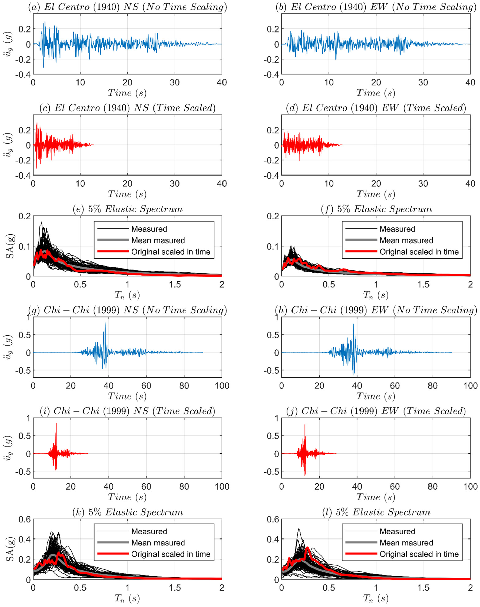
(a), (b), (g), and (h) 1940 El Centro and 1999 Chi-Chi CHY080 recorded ground motions. (c), (d), (i), and (j) Recorded ground motions’ scaled in time by 3.11. (e), (f), (k), and (l) Measured, mean measured, and original ground motions’ 5%-damped elastic acceleration response spectra.

Ground motion scaling

The mass of the rocking body originates both the stabilizing (self-weight) and the destabilizing (inertia) elements of Housner’s rocking body model (Housner, 1963), which is dimensionally analogous to the elementary pendulum model. Thus, the acceleration scale must be preserved to design the experiments, implying that the time scale, S_T, should be equal to the square of the geometrical scaling of the specimen S_L (i.e. $S_{T} = \sqrt{S_{L}}$ ). Since the ground motion ensembles were generated to be consistent with the target elastic response spectra of two “seed” recorded ground motions, the size of the wobbling specimen was related to the size of the columns in a bridge prototype structure (taken here as 9.67 m) to determine a length scale S_L (equal to 1/9.67 in this case). This means that the time component of the generated ground motions was scaled by a factor of $\sqrt{9.67}$ = 3.11, that is, the frequency of ground motions was increased without changing the amplitude. Figure 4 (e, f, k, and l) plots the 5%-damped elastic response spectra of the motions, as applied by the shake table and measured using an accelerometer installed on the shaking table platform. Note that for this plot, the measured acceleration recordings of the offered dataset were further processed so that they have zero final velocity: the mean of the record was subtracted from each element of that record.

It should be noted that the wobbling specimen at hand is only a distorted model of a prototype structure because stress similitude is not preserved. This is typical in scaling problems where similitude cannot be retained for all problem variables. Thus, the elastic modulus of the material and the natural frequencies of the prototype are not faithfully scaled. In addition, the wobbling specimen columns are not perfectly rigid, as Vassiliou (2018) assumes, while compliant foundation conditions and the associated soil–structure interaction effects are ignored (e.g. kinematic interaction, radiation damping, rotational base excitation, permanent settlement, and tilting) (NEHRP Consultants Joint Venture, 2012). However, it has been shown that the deformability of large structures does not qualitatively change their rocking behavior (Acikgoz and DeJong, 2012; Chopra and Yim, 1985; Ma, 2010; Oliveto et al., 2003; Psycharis, 1991; Truniger et al., 2015; Vassiliou et al., 2014, 2015). Furthermore, the ends of the columns of a real rocking podium structure would be protected from localized damage, and are likely to remain elastic during seismic response. Ultimately, the conducted experiments are deemed adequately realistic for studying the statistical properties of wobbling columns and create a useful and reliable benchmark dataset for wobbling seismic response model validation without aiming to represent the nuances of a prototype structure without distortion.

Testing protocol

The first 100 El Centro tests are denoted as N1 to N100. Within this subset, the tests that seem to have excited the system the most were N79, N83, N92, N96, and N97. The next 100 Chi-Chi tests are denoted as N101 to N200. In this subset, the following tests caused the most substantial excitation in the table top: N113, N114, N174, N180, N181, N188, N189, N190, N195, N196, N197, and N199.

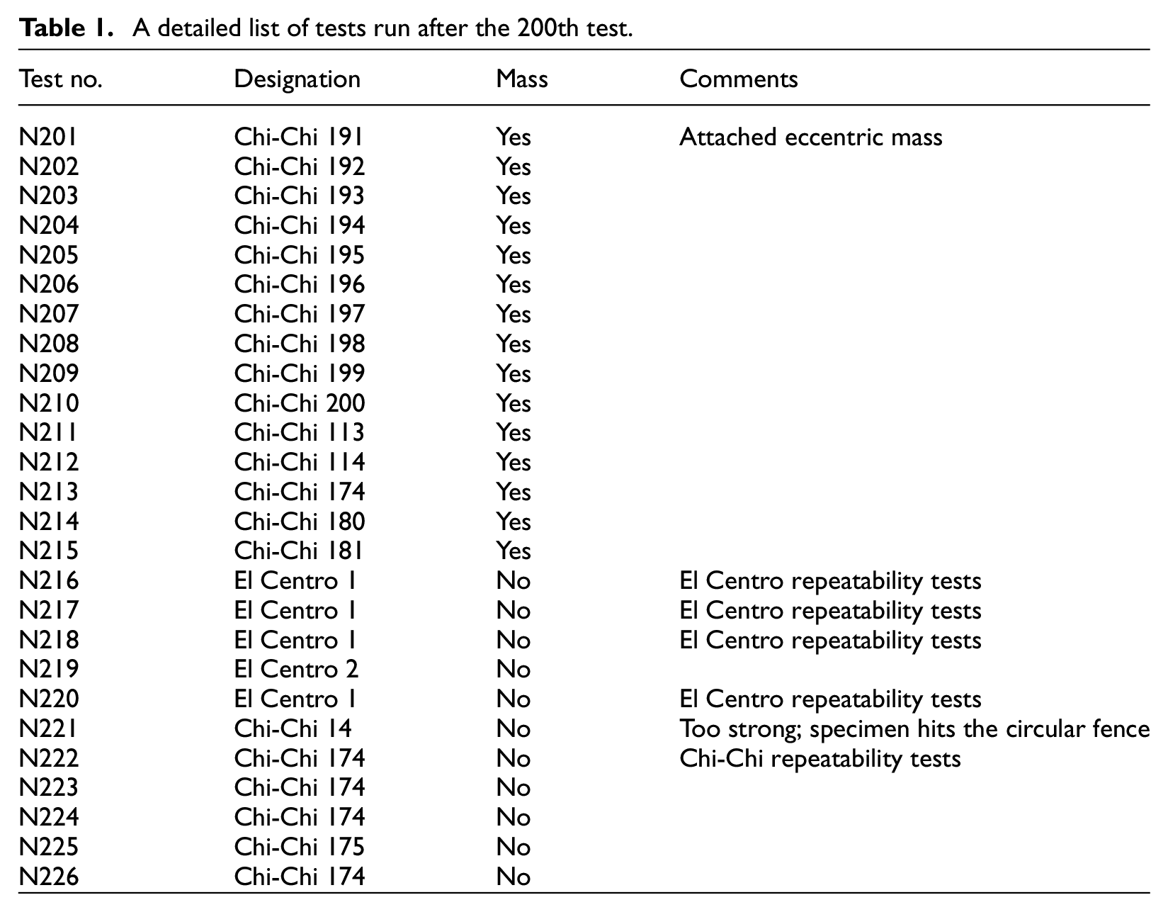
After running these 200 ground motions, a mass of 80 ± 0.25 kg (which corresponds to a 13% increase of the mass supported by the columns) was attached above column 4 (Figure 5). This column is the right one shown in Figure 6 below point M6. The purpose of the added mass is to alter the inertia distribution and create a degree of eccentricity. In practice, this eccentricity aims to represent the case of eccentrically distributed live load on the deck of a bridge, which is quite common when earthquakes occur during operational conditions. Tests denoted as N201–N215 were run with the mass attached. As some of the largest motions were observed in tests N191–N200, these 10 motions were applied in the eccentric model. In addition, motions N113, N114, N174, N180, and N181 were also run, because they induced some of the largest specimen motions in this testing campaign. Table 1 summarizes the excitations used for the eccentric specimen. Following the tests of the wobbling specimen with the eccentric mass, the mass was removed and repeatability tests using the original symmetric wobbling specimen, denoted as N216–N226 in Table 1, were conducted. It is worth noting that at no point was the structure reconfigured, repaired, or resettled.

Table 1.

A detailed list of tests run after the 200th test.

Test no.	Designation	Mass	Comments
N201	Chi-Chi 191	Yes	Attached eccentric mass
N202	Chi-Chi 192	Yes
N203	Chi-Chi 193	Yes
N204	Chi-Chi 194	Yes
N205	Chi-Chi 195	Yes
N206	Chi-Chi 196	Yes
N207	Chi-Chi 197	Yes
N208	Chi-Chi 198	Yes
N209	Chi-Chi 199	Yes
N210	Chi-Chi 200	Yes
N211	Chi-Chi 113	Yes
N212	Chi-Chi 114	Yes
N213	Chi-Chi 174	Yes
N214	Chi-Chi 180	Yes
N215	Chi-Chi 181	Yes
N216	El Centro 1	No	El Centro repeatability tests
N217	El Centro 1	No	El Centro repeatability tests
N218	El Centro 1	No	El Centro repeatability tests
N219	El Centro 2	No
N220	El Centro 1	No	El Centro repeatability tests
N221	Chi-Chi 14	No	Too strong; specimen hits the circular fence
N222	Chi-Chi 174	No	Chi-Chi repeatability tests
N223	Chi-Chi 174	No
N224	Chi-Chi 174	No
N225	Chi-Chi 175	No
N226	Chi-Chi 174	No

Figure 5.

Extra mass added on top of column 4 to create eccentricity.

Figure 6.

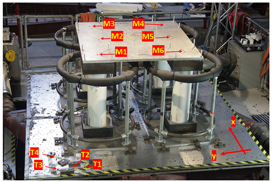
Marker positions on top of the aluminum slab (M1–M6) and on the shake table (T1–T4) used for wobbling specimen displacement measurements.

Instrumentation

Infrared vision tracking and acceleration measurements

The displacements were measured using a set of 10 infrared markers shown in Figure 6, including the coordinate system. The position of the markers was tracked using a Qualisys AB (2006) high-resolution infrared tracking system comprising five infrared cameras. Four of these were mounted around the table and the fifth one was on the overhanging beam, making it possible to capture each marker with at least two infrared cameras at all times. Six markers were installed on the top of the aluminum slab of the wobbling specimen.

These six markers can capture the motion along the six degrees of freedom of the slab (three translations and three rotations), assuming it remains rigid, which is a fair assumption for the case studied. Markers M1, M3, M4, and M6 lie on the axial projections of columns C1, C2, C3, and C4 axes, respectively. Markers M2 and M5 are redundant intermediate markers. When the extra mass was added to create eccentricity, Marker M6 was placed on top of the mass again at the projection of the column axis. The shaking table motion is tracked with four markers denoted as T1, T2, T3, and T4. The sampling rate was 100 Hz.

The acceleration of the shaking table was monitored by a block of mutually orthogonal accelerometers. The acquired acceleration data, sampled at 5000 Hz, was filtered using a low-pass 8-pole Butterworth filter with a cut-off frequency set at 1400 Hz. The two data acquisition systems, for displacements and accelerations, are triggered and synchronized via a common clock signal.

Photos and videos

Photos of the specimen were taken before, during, and after the tests (i.e. at rest) to record the potential damage caused by uplifting, minor sliding, and impact of the specimens. Videos of all tests were also recorded.

Test observations

A noteworthy observation made is that the bevels (conic end restraints) had a very fine layer of steel dust after the Chi-Chi test series, as seen in Figure 3. It seems that the steel dust was caused by the “climbing” of the columns on the incline of the bevels. Some markings on the inner surface of the bevels were observed, and some of those markings were very close to the top of the bevels. This observation was made for the bevels attached to the table top, suggesting that the table top was lifted at times as much as 110 mm. There were no visible indentations on the inclined surfaces except for some very fine lines or scratches (Figure 3). It is notable that, no such markings or ground-down steel materials were found after the first 100 El Centro tests.

Upon completion of tests and disassembly of the experimental model, it was noticed that the top pegs (aluminum circular stoppers) had detached from the conical end restraints (Figure 7). The peg height and diameter (Figure 2) were designed such that they do not engage until the tilt angle of the columns, computed assuming that the columns do not “climb” on the conical bevels, is larger than the static overturning angle of the wobbling specimen. Thus, the only conceivable way that the pegs could have engaged is the case where the columns indeed “climbed” on the bevels and changed the specimen geometry—as confirmed by the markings observed on the conical restraints (Figure 3). Therefore, it is not clear whether not observing overturning is a consequence of possible pegs engagement, the columns climbing on the conical bevels, or the insufficiently high intensity of the applied ground motions.

Figure 7.

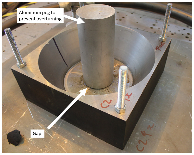
The gap between the aluminum peg and the bottom of the conical end restraint, observed after the tests, indicates the column engaged the peg.

During the test, the table was commanded to move only in the horizontal plane. However, due to the workings of the shaking table control system, there are small and unavoidable vertical motions. This is why the recorded accelerations in the vertical (z) direction are not zero.

However, the spikes in the vertical acceleration graphs (Figures 9 and 10, bottom-right) are significantly larger than the vertical accelerations induced by the shaking table. These spikes might correspond to vertical accelerations caused by the impact of the specimen on the table during rocking.

Test data

Organization of the data

The test data can be downloaded from the publicly accessible ETH Research Collection platform (Vassiliou et al., 2020b), where they are indefinitely maintained.

The dataset comprises four files, compressed using the ZIP format, containing (1) the measurements of the position of the markers (from which the displacements can be computed), (2) the acceleration measurements, (3) the test videos, and (4) photos of the specimens. It should be noted that for tests N3 and N158, the accelerometers did not start, so there was no recording of the acceleration for these tests. Therefore, there are 224 complete, acceleration and position, files. The structure of the data files is summarized in Figure 8.

Figure 8.

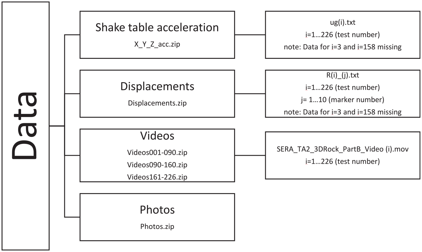
Data organization and file naming convention.

Displacement data

Marker position time histories are provided as ASCII files named Ri_j.txt. Each file comprises three columns, corresponding to the position of the marker along the x, y, and z directions of the coordinate system shown in Figure 6. The table platen is horizontal, and in the x–y plane of this coordinate system. The position units are millimeters. Index i denotes the test number. Index j denotes the marker/target number: j = 1–4 are the markers placed on the shake table (i.e. targets Tj in Figure 6), while markers j = 5–10 are placed on the aluminum slab (i.e. M(j-4) in Figure 6). The data are sampled at 100 Hz and processed by the Qualisys system.

Acceleration data

The filtered acceleration time histories record in 224 (226 minus tests N3 and N158) tests are provided as ASCII files, named i.txt, where i ={test number}. Within each file, the first, second, and third columns are the accelerations in the x, y, and z directions of the coordinate system shown in Figure 6, respectively, in units of acceleration of gravity (g). The acceleration data were not corrected in any way.

Data synchronization

The date and time data for each test are provided in ASCII files named TimeStampi.txt, where i = {test number}. The two data acquisition systems, for displacements and accelerations, are triggered and synchronized via a common clock signal.

Examples of derived data

Throughout this section, the displacements of the shake table were computed using the position of target T1 (Figure 6). The displacement of target T1 should, in theory, be equal to the position of targets T2, T3, and T4, as no rotations were commanded to the shake table. However, unavoidably, the table did experience some small rotations that resulted in small deviations between displacements of targets T1, T2, T3, and T4.

Figures 9 and 10 plot the orbits of the horizontal displacements of markers M1, M3, M4, and M6 relative to the shake table displacement for the N1 (El Centro #1) and the N101 (Chi-Chi #1) tests, respectively. It also plots the three components of the acceleration, as recorded and filtered with a low-pass filter, but without correcting them for non-zero mean. Had the wobbling specimen and the shake table excitation been perfect, the displacements of all markers, M1–M6, would have been the same. However, the unavoidable imperfections present in the tests resulted in rotations of the wobbling specimen slab around the vertical axis (twisting of the specimen).

Figure 9.

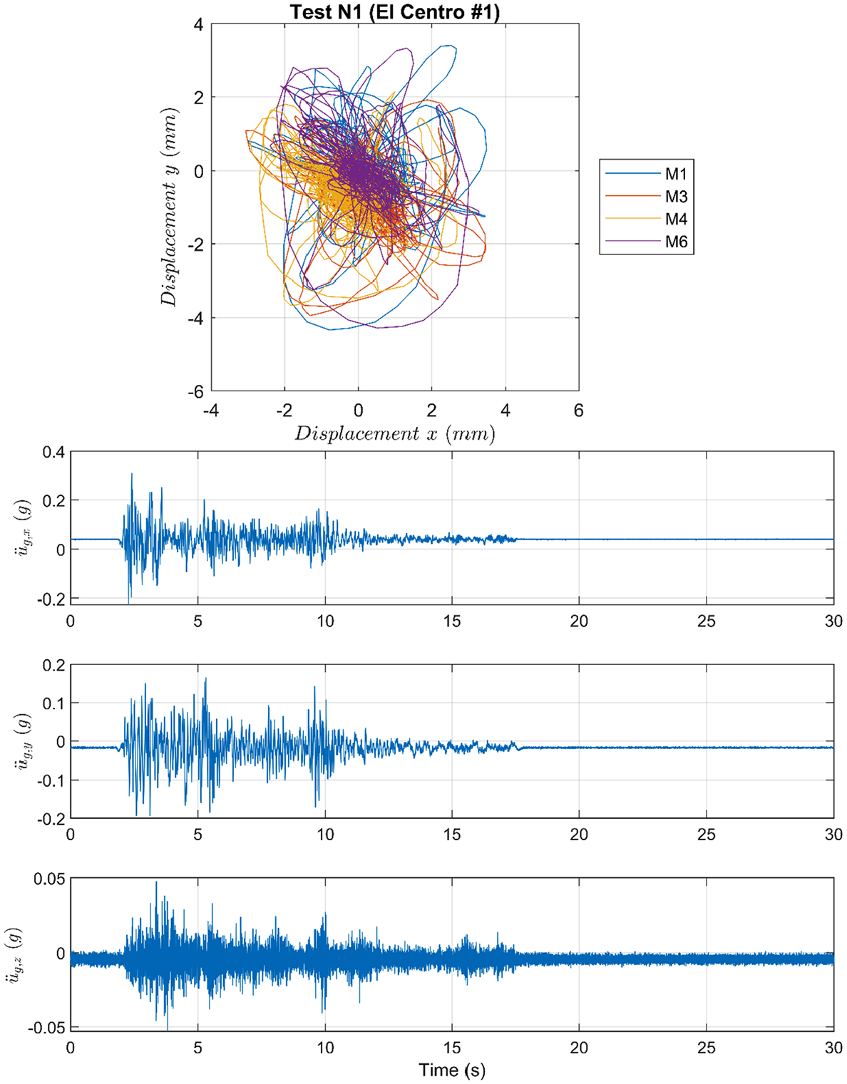
Row 1: Orbits of the horizontal displacements of markers M1, M3, M4, and M6; Rows 2–4: Recorded acceleration in x, y, and z directions; Test N1.

Figure 10.

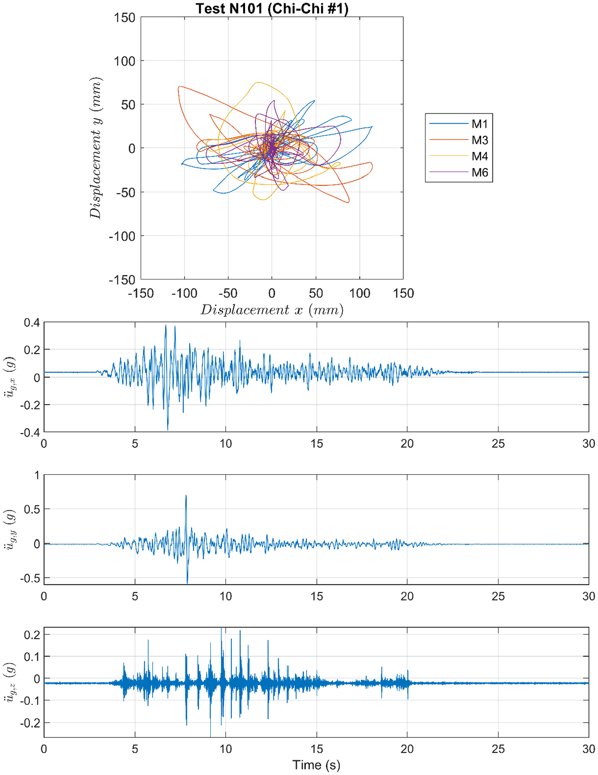
Row 1: Orbits of the horizontal displacements of markers M1, M3, M4, and M6; Rows 2–4: Recorded acceleration in x, y, and z directions; Test N101.

It is also notable that both the maximum and the residual displacements and maximum accelerations induced by the El Centro #1 ground motions are significantly smaller than those induced by the Chi-Chi #1 motion. This is why different scales are used in the two sets of plots.

Figure 11 plots the same marker displacement quantities for tests N192 and N202 to show the influence of the added eccentric mass. It seems that the addition of the mass does not significantly influence the response (at least in terms of maximum quantities), because the center of mass and the center of rigidity are affected similarly.

Figure 11.

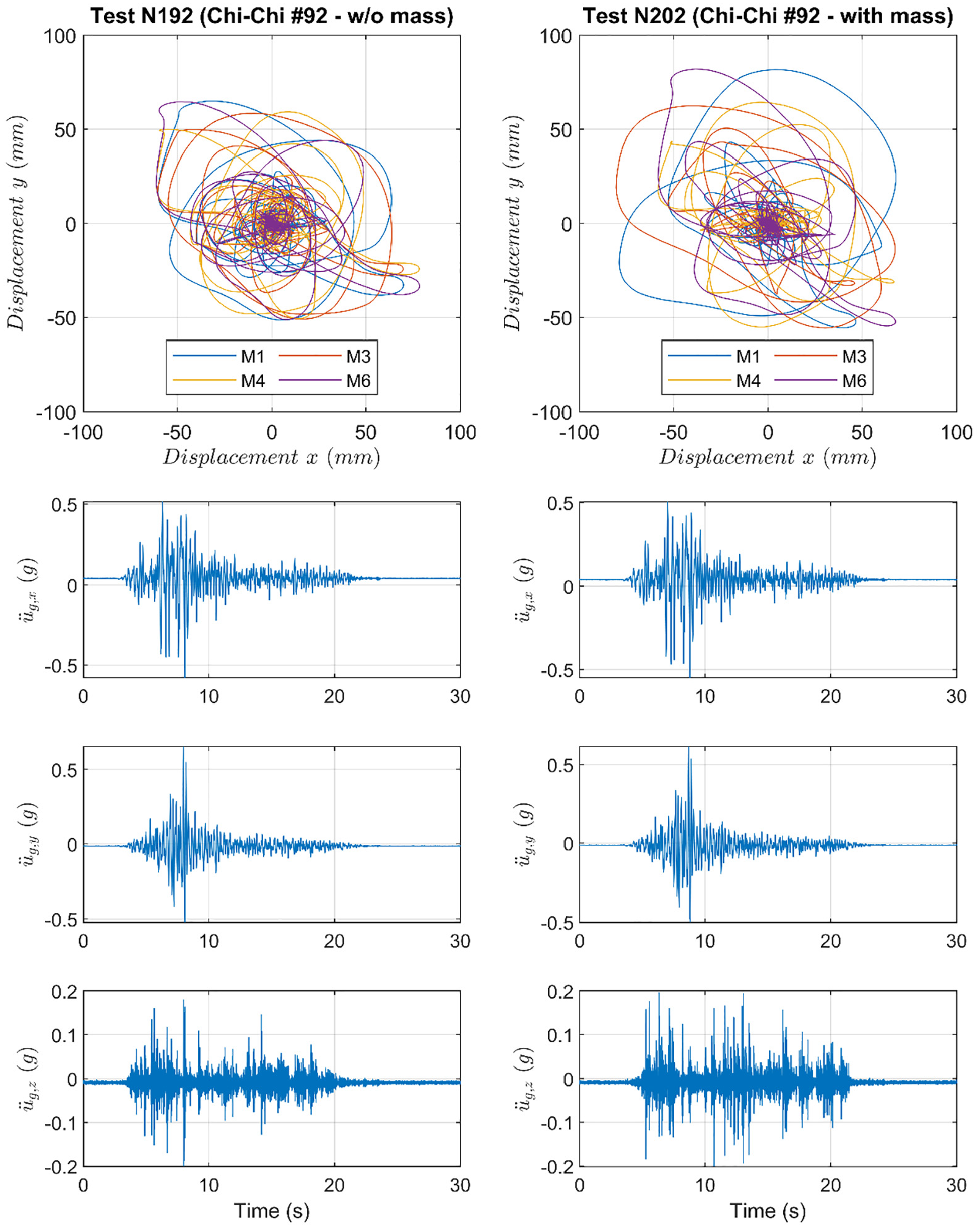
Row 1: Orbits of the horizontal displacements of markers M1, M3, M4, and M6; Rows 2–4: Recorded acceleration in x, y, and z directions; Left: Test N192 (w/o eccentric mass); Right Test N101 (with eccentric mass).

Figures 12 and 13 plot the outcomes of four repeatability tests for the El Centro #1 (left column) and Chi-Chi #174 (right column) ground motions. Repeatability is not observed.

Figure 12.

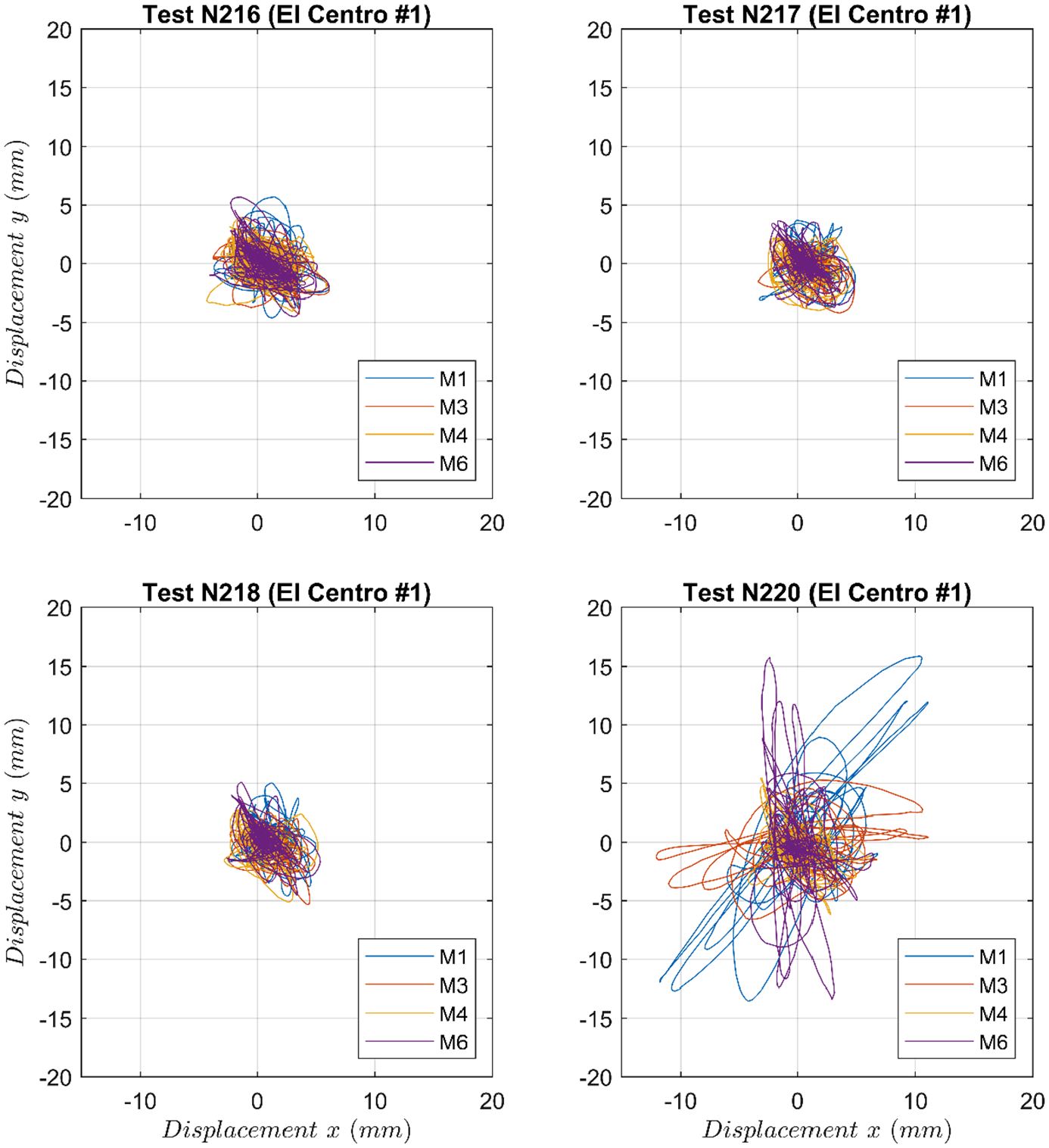
Repeatability test for El Centro #1 excitation: Orbits of the horizontal displacements of markers M1, M3, M4, and M6.

Figure 13.

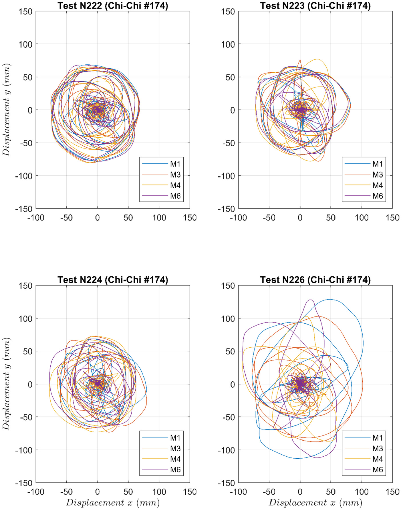
Repeatability test for Chi-Chi #1 excitation: Orbits of the horizontal displacements of markers M1, M3, M4, and M6.

Data use

The main purpose of the generated dataset is to enable the validation of analytical and numerical models for seismic response of 3D uplifting structures that wobble, that is, 3D motion characterized by simultaneous uplift from the ground (rocking) and change of the contact point with the ground (nutation) without spinning or sliding out of its original position (van den Engh et al., 2000; Vassiliou, 2018; Vassiliou et al., 2017a). Improving the numerical models will reduce the epistemic uncertainty and will allow for better prediction of the response of wobbling structures that can in turn enhance their applicability in earthquake engineering applications. The data presented herein have been used in the PEER 2019 blind prediction contest, the results of which have been published in the work of Vassiliou et al. (2020a). This was the first blind prediction contest where the participants were asked to predict the statistics of the response to sets of ground motions, thus illustrating the importance of the statistical approach in validating models used in earthquake engineering and the significance of the dataset at hand.

The experience from the PEER 2019 blind prediction contest indicates that the data presented herein can be used for two additional purposes. One is to compare modeling approaches (e.g. analytical models based on rigid or flexible rocking body assumptions, finite element method models, discrete element method models) and to determine the relative importance of different parameters used in each of these approaches. The other is to compare different approaches to model energy dissipation (e.g. restitution coefficients) in wobbling structures in particular, and in uplifting structures in general, resting on a rigid base.

Moreover, validating numerical models used for rocking structure models can be used for the study of museum artifacts, statues, and the behavior of other precious unanchored equipment.

Conclusion

This article described the publicly available data obtained from a series of 226 shake table tests of a 3D rocking podium structure. The structure, designed at ETH Zurich and built in Bristol, represents bridge or building structures whose columns uplift from their bases when the structures are subjected to an earthquake. The tests were performed at the EQUALS of University of Bristol. The purpose of the presented data is to serve a benchmark response dataset for statistical validation of numerical models intended to predict the seismic response of rocking structures. Additional insights on the overall stability and the recovery capability of the wobbling specimen were obtained. The authors hope this dataset and its use to validate seismic response models for rocking and wobbling structures will accelerate their adoption in practice.

Footnotes

Acknowledgements

The authors would also like to acknowledge the contribution of the personnel at EQUALS laboratory, University of Bristol.

Declaration of conflicting interests

The author(s) declared no potential conflicts of interest with respect to the research, authorship, and/or publication of this article.

Funding

The author(s) disclosed receipt of the following financial support for the research, authorship, and/or publication of this article: This research was conducted as part of the transnational access project “Statistical verification and validation of 3D seismic rocking motion models (3DROCK)” funded by the EC H2020 under grant agreement number 730900 (SERA: Seismology and Earthquake Engineering Research Infrastructure Alliance for Europe, ).

ORCID iDs

Cihan Cengiz

George Mylonakis

Bozidar Stojadinovic

References

Acikgoz

DeJong

(2012) The interaction of elasticity and rocking in flexible structures allowed to uplift. Earthquake Engineering & Structural Dynamics 41(15): 2177–2194.

Agalianos

Psychari

Vassiliou

Stojadinovic

Anastasopoulos

(2017) Comparative assessment of two rocking isolation techniques for a motorway overpass bridge. Frontiers in Built Environment 3: 47.

Anagnostopoulos

Norman

Mylonakis

(2019) Fractal like overturning maps for stacked rocking blocks with numerical and experimental validation. Soil Dynamics & Earthquake Engineering 125: 105659.

Bachmann

(2018) Development of self-centering systems with geometry-controlled stiffness for earthquake hazard mitigation. Doctoral Dissertation, ETH Zurich, Zurich, Switzerland.

Bachmann

Strand

Vassiliou

Broccardo

Stojadinovic

(2019a) Modelling of rocking structures: Are our models good enough? In: 2nd international conference on natural hazards & infrastructure (ICONHIC 2019), Chania, Crete, 23–26 June.

Bachmann

Strand

Vassiliou

Broccardo

Stojadinovic

(2018) Is rocking motion predictable? Earthquake Engineering & Structural Dynamics 47(2): 535–552.

Bachmann

Vassiliou

Stojadinović

(2017) Dynamics of rocking podium structures. Earthquake Engineering & Structural Dynamics 46(14): 2499–2517.

Bachmann

Vassiliou

Stojadinovic

(2019b) Rolling and rocking of rigid uplifting structures. Earthquake Engineering & Structural Dynamics 48(14): 1556–1574.

Bao

Konstantinidis

(2020) Dynamics of a sliding-rocking block considering impact with an adjacent wall. Earthquake Engineering & Structural Dynamics 49(5): 498–523.

10.

Broccardo

Dabaghi

(2017) A spectral-based stochastic ground motion model with a non-parametric time-modulating function. In: 12th international conference on structural safety and reliability, Vienna, 6–17 August, pp. 1–10.

11.

Broccardo

Der Kiureghian

(2014) Simulation of near-fault ground motions using frequency-domain discretization. In: Proceedings of the 10th national conference on earthquake engineering, Anchorage, AK, 21–25 July.

12.

Cherepinskiy

(2004) Seismic isolation of buildings with application of the kinematics bases. In: 13th world conference on earthquake engineering, Vancouver, BC, Canada, 1–6 August.

13.

Chopra

Yim

SCS

(1985) Simplified earthquake analysis of structures with foundation uplift. Journal of Structural Engineering 111(4): 906–930.

14.

Dar

Konstantinidis

El-Dakhakhni

(2018) Seismic response of rocking frames with top support eccentricity. Earthquake Engineering & Structural Dynamics 47(12): 2496–2518.

15.

Dar

Konstantinidis

El-Dakhakhni

(2016) Evaluation of ASCE 43-05 seismic design criteria for rocking objects in nuclear facilities. Journal of Structural Engineering 142(11): 04016110.

16.

Del Giudice

Wrobel

Leinenbach

Vassiliou

(2020) Static testing of additively manufactured microreinforced concrete specimens for statistical structural model validation at a small scale. In:8th international conference on advances in experimental structural engineering (8AESE), Christchurch, New Zealand, 3–5 February.

17.

Di Egidio

Alaggio

Contento

Tursini

Della Loggia

(2015) Experimental characterization of the overturning of three-dimensional square based rigid block. International Journal of Non-Linear Mechanics 69: 137–145.

18.

Di Sarno

Magliulo

D’Angela

Cosenza

(2019) Experimental assessment of the seismic performance of hospital cabinets using shake table testing. Earthquake Engineering & Structural Dynamics 48(1): 103–123.

19.

Dimitrakopoulos

Giouvanidis

(2015) Seismic response analysis of the planar rocking frame. Journal of Engineering Mechanics 141(7): 04015003.

20.

Housner

(1963) The behavior of inverted pendulum structures during earthquakes. Bulletin of the Seismological Society of America 53(2): 403–417.

21.

Konstantinidis

Makris

(2010) Experimental and analytical studies on the response of 1/4-scale models of freestanding laboratory equipment subjected to strong earthquake shaking. Bulletin of Earthquake Engineering 8(6): 1457–1477.

22.

QTM

(2010) The mechanics of rocking structures subjected to ground motion. Doctoral Dissertation, ResearchSpace@, Auckland, New Zealand.

23.

Makris

Vassiliou

(2013) Planar rocking response and stability analysis of an array of free-standing columns capped with a freely supported rigid beam. Earthquake Engineering & Structural Dynamics 42(3): 431–449.

24.

Makris

Vassiliou

(2014) Are some top-heavy structures more stable? Journal of Structural Engineering 140(5): 06014001.

25.

NEHRP Consultants Joint Venture (2012) Soil-Structure Interaction for Building Structures (Report NIST/GCR 11-917-14). Washington, DC: Applied Technology Council and Consortium of Universities for Research in Earthquake Engineering for the National Institute of Standards and Technology.

26.

Oliveto

Calio

Greco

(2003) Large displacement behaviour of a structural model with foundation uplift under impulsive and earthquake excitations. Earthquake Engineering & Structural Dynamics 32(3): 369–393.

27.

Psycharis

(1991) Effect of base uplift on dynamic response of SDOF structures. Journal of Structural Engineering 117(3): 733–754.

28.

Qualisys

(2006) Qualisys Track Manager User Manual. Gothenburg: Qualisys AB.

29.

Rezaeian

Der Kiureghian

(2008) A stochastic ground motion model with separable temporal and spectral nonstationarities. Earthquake Engineering & Structural Dynamics 37(13): 1565–1584.

30.

Ríos-García

Benavent-Climent

(2020) New rocking column with control of negative stiffness displacement range and its application to RC frames. Engineering Structures 206: 110133.

31.

Sextos

Manolis

Ioannidis

Athanasiou

(2017) Seismically induced uplift effects on nuclear power plants. Part 2: Demand on internal equipment. Nuclear Engineering and Design 318: 288–296.

32.

Shaking Table Specifications (n.d.). http://www.bris.ac.uk/engineering/research/earthquakegeo/equip/tablespec/ (accessed 29 April 2020).

33.

Truniger

Vassiliou

Stojadinović

(2015) An analytical model of a deformable cantilever structure rocking on a rigid surface: Experimental validation. Earthquake Engineering & Structural Dynamics 44(15): 2795–2815.

34.

Uzdin

Doronin

Davydova

Avidon

Karlina

(2009) Performance analysis of seismic-insulating kinematic foundations on support elements with negative stiffness. Soil Mechanics and Foundation Engineering 46(3): 99–107.

35.

van den Engh

Nelson

Roach

(2000) Numismatic gyrations. Nature 408(6812): 540–540.

36.

Vassiliou

(2018) Seismic response of a wobbling 3D frame. Earthquake Engineering & Structural Dynamics 47(5): 1212–1228.

37.

Vassiliou

Broccardo

Cengiz

Dietz

Dihoru

Gunay

Mosalam

Mylonakis

Sextos

Stojadinovic

(2020a) Shake table testing of a rocking podium: Results of a blind prediction contest. Earthquake Engineering and Structural Dynamics. Epub ahead of print 10 November. DOI: 10.1002/eqe.3386.

38.

Vassiliou

Burger

Egger

Bachmann

Broccardo

Stojadinovic

(2017a) The three-dimensional behavior of inverted pendulum cylindrical structures during earthquakes. Earthquake Engineering & Structural Dynamics 46(14): 2261–2280.

39.

Vassiliou

Cengiz

Dietz

Dihoru

Broccardo

Mylonakis

Sextos

Stojadinovic

(2020b) Dataset from the shake table tests of a rocking podium structure. ETH Research Collection Platform. DOI: 10.3929/ethz-b-000429931.

40.

Vassiliou

Mackie

Stojadinović

(2014) Dynamic response analysis of solitary flexible rocking bodies: Modeling and behavior under pulse-like ground excitation. Earthquake Engineering & Structural Dynamics 43(10): 1463–1481.

41.

Vassiliou

Mackie

Stojadinović

(2017b) A finite element model for seismic response analysis of deformable rocking frames. Earthquake Engineering & Structural Dynamics 46(3): 447–466.

42.

Vassiliou

Truniger

Stojadinović

(2015) An analytical model of a deformable cantilever structure rocking on a rigid surface: Development and verification. Earthquake Engineering & Structural Dynamics 44(15): 2775–2794.

43.

Voyagaki

Kloukinas

Dietz

Dihoru

Horseman

Oddbjornsson

Crewe

Taylor

Steer

(2018) Earthquake response of a multiblock nuclear reactor graphite core: Experimental model vs simulations. Earthquake Engineering & Structural Dynamics 47(13): 2601–2626.

44.

Wittich

Hutchinson

(2015) Shake table tests of stiff, unattached, asymmetric structures. Earthquake Engineering & Structural Dynamics 44(14): 2425–2443.