Regional attenuation models in Central and Eastern North America using the NGA-East database

Abstract

The anelastic attenuation term found in ground motion prediction equations (GMPEs) represents the distance dependence of the effect of intrinsic and scattering attenuation on the wavefield as it propagates through the crust and contains the frequency-dependent quality factor, $Q (f)$ , which is an inverse measure of the effective anelastic attenuation. In this work, regional estimates of $Q (f)$ in Central and Eastern North America (CENA) are developed using the NGA-East regionalization. The technique employed uses smoothed Fourier amplitude spectrum (FAS) data from well-recorded events in CENA as collected and processed by NGA-East. Regional $Q (f)$ is estimated using an assumption of average geometrical spreading applicable to the distance ranges considered. Corrections for the radiation pattern effect and for site response based on $V_{s 30}$ result in a small but statistically significant improvement to the residual analysis. Apparent $Q (f)$ estimates from multiple events are combined within each region to develop the regional models. Models are provided for three NGA-East regions: the Gulf Coast, Central North America, and the Appalachian Province. Consideration of the model uncertainties suggests that the latter two regions could be combined. There were not sufficient data to adequately constrain the model in the Atlantic Coastal Plain region. Tectonically stable regions are usually described by higher $Q (f)$ and weaker frequency dependence ( $η$ ), while active regions are typically characterized by lower $Q (f)$ and stronger frequency dependence, and the results are consistent with these expectations. Significantly different regional $Q (f)$ is found for events with data recorded in multiple regions, which supports the NGA-East regionalization. An inspection of two well-recorded events with data both in the Mississippi embayment and in southern Texas indicates that the Gulf Coast regionalization by Cramer in 2017 may be an improvement to that of NGA-East for anelastic attenuation. The $Q (f)$ models developed serve as epistemic uncertainty alternatives in CENA based on a literature review and a comparison with previously published models.

Keywords

Ground motion attenuation quality factor CENA stochastic method seismic hazard

Introduction

In tectonically active regions of the United States, such as California, the seismicity rates are sufficient such that design ground motions can be estimated using empirical ground motion prediction equations (GMPEs, also called ground motion models, GMMs). However, for areas with low rates of seismicity, such as Central and Eastern North America (CENA), it is challenging to develop empirical GMPEs because very few data exist, and most are for small magnitude earthquakes. Although they are infrequent, the potential for large earthquakes exists in CENA; therefore, developing GMPEs for this region requires alternative methods beyond empirical modeling. Substantial effort has been made on this topic, including Boore and Atkinson (1987), Electric Power Research Institute (EPRI, 1993), Toro et al. (1997), Silva et al. (2002), Abrahamson and Silva (2001), Atkinson (2012), and most recently, the collaborative effort of the Pacific Earthquake Engineering Research Center’s NGA-East (PEER, 2015; NGA-East hereafter).

When deriving GMPEs in data-poor regions, several alternatives exist, but earthquake simulations are widely used for supplementing the recorded data. Over the last several decades, the stochastic point-source method has been the commonly used simulation method for this purpose. The stochastic method is based on the pioneering work of Brune (1970, 1971), Hanks and McGuire (1981), and Boore (1983), among others. David Boore extended it to the simulation of acceleration time series in Boore (1983) and Boore (2003). Following Boore (2003), a simulated time series is produced using a seismological model of the Fourier amplitude spectrum (FAS), and assuming the spectrum is distributed with random phase angles over a time duration related to the earthquake magnitude and the distance between the source and site. For more details on the stochastic method, the reader is referred to Supplemental Appendix 3A of the NGA-East Report (PEER, 2015) or to Boore (2003), both of which give excellent descriptions.

Details in the application of this method vary, but the conventional stochastic method uses an omega-square source model (Brune, 1970, 1971) with a single-corner frequency and a constant stress drop (Atkinson, 1984; Boore, 1983), in which the shape of the acceleration FAS spectral density $Y$ at frequency $f$ is given by equation 1,

\begin{matrix} Y (f) = \hat{C} \frac{f^{2}}{1 + {(\frac{f}{f_{0}})}^{2}} M_{0} A (f) D (f) G (R) \exp (\frac{- π fR}{Q (f) β_{0}}) \end{matrix}

Equation 1

where $f$ is the frequency, $M_{0}$ is seismic moment, $R$ is the effective source–site distance, $f_{0}$ is the source corner frequency (related to the seismic moment and stress drop, $Δ σ$ ), $β_{0}$ is the shear wave velocity near the source, $A (f)$ is the crustal amplification, $D (f)$ is the high-frequency diminution term (kappa or f_max term), $G (R)$ is the geometric spreading function (1/ $R$ for a uniform whole space), and $\hat{C}$ is a constant that accounts for the source region material density, the effect of the free surface, averaged source radiation pattern, and the partition of energy into two horizontal components. The final exponential term represents the distance dependence of the effect of intrinsic and scattering attenuation on the wavefield as it propagates through the crust. The quality factor, $Q (f)$ , is an inverse measure of effective anelastic attenuation, which introduces a decay in spectral amplitudes with distance; this attenuation is frequency-dependent, and thus alters spectral shape (Atkinson and Boore, 2014). The purpose of this study is to develop improved regional estimates of $Q (f)$ in CENA.

Taking the natural logarithm ( $\ln$ ) of both sides of equation 1 and using the product rule of logarithms yield equation 2. The form of this equation resembles the basic form of many GMPEs for the median ground motion, for example, equation 3. $Source$ is a collection of earthquake source-related terms generally described by moment magnitude (M) and style of faulting, $Site$ is a collection of site amplification terms (often parameterized by $V_{s 30}$ and basin depths), $b$ is the frequency-independent geometric spreading coefficient, and $c (f)$ is the coefficient of anelastic attenuation. From equations 2 and 3, the relationship between $c (f)$ and $Q (f)$ is determined.

\begin{matrix} \ln [Y (f)] = \ln [\hat{C} \frac{f^{2}}{1 + {(\frac{f}{f_{0}})}^{2}} M_{0}] + \ln [A (f) D (f)] + \ln [G (R)] + (\frac{- π fR}{Q (f) β_{0}}) \end{matrix}

Equation 2

\begin{matrix} \ln [Y (f)] = Source (f) + Site (f) + b \ln [R] + c (f) R \end{matrix}

Equation 3

$Q (f)$ is believed to be attributable to intrinsic absorption, plus the frequency-dependent effects of scattering (Atkinson, 2012; Dainty, 1981), and is usually modeled with the form $Q (f) = Q_{0} f^{η}$ , where $Q_{0}$ is the $Q$ value at 1 Hz, and $η$ is the slope parameter. The geometric attenuation ( $b$ term) models the amplitude decay due to the expanding surface area of the wave front as it propagates away from the source and generally controls the attenuation of ground motions at near source distances. At distances greater than about 100 km, the anelastic attenuation effects, which are frequency-dependent, become dominant (Atkinson, 2012). This is evident in equation 3, for which the geometric spreading attenuation scales with $\ln (R)$ and the anelastic attenuation scales with $R$ . However, the geometric spreading and anelastic attenuation are coupled, and empirical studies have shown that the same data can be fit (for particular M and distance ranges) with different trade-offs between parameters $b$ and $c$ . Therefore, suites of parameters developed empirically are relative to each other, and care must be taken when separately evaluating one term from one study, with another from another study.

Previous work

Previous studies of regional CENA attenuation models are numerous; recent works include Cramer (2017), Cramer and Al Noman (2016), Bisrat et al. (2014), Yassminh et al. (2020), Chapman and Conn (2016), Guo and Chapman (2019), Pasyanos (2013), Gallegos et al. (2014), and NGA-East (PEER, 2015). The NGA-East project was a multi-disciplinary research project managed by Christine Goulet with the objective to develop a new ground motion characterization (GMC) model for CENA. Part of this project was to develop median GMPEs for the region, and this task included eight categories of approaches, split into 10 chapters, with a different GMPE (and authors) for each chapter. Six of these chapters utilize some variation of stochastic method modeling and therefore, have either adopted or inverted models for $Q (f)$ . As a starting point for NGA-East, Goulet et al. (2015) compiled attenuation (geometric spreading and anelastic attenuation) models from the literature; over 40 were identified and after review, six high quality models were selected to span the range of available models while maintaining a manageable number of models. These are summarized in Table 2.1 of Boore (2015). The attenuation models (geometrical spreading and anelastic attenuation) used with stochastic method simulations as part of the NGA-East project are used as the basis for comparisons in the section titled “Model comparison.”

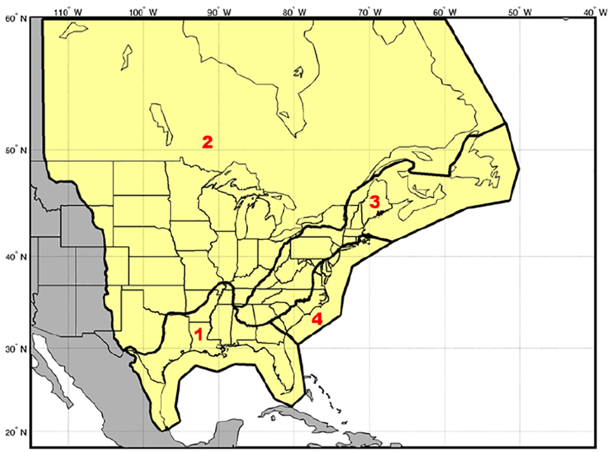
Cramer (2017) and Cramer and Al Noman (2016) studied boundaries between major $Q$ regions in the continental United States using the Earthscope USArray data. This was accomplished using transects of observations across the transitions to look for major changes in $Q$ . In this process, Cramer and Al Noman (2016) determined regional estimates of apparent $Q$ ; these are also used as the basis for comparisons in this article. The Cramer (2017) Gulf Coast $Q$ northern boundary roughly corresponds to the Alabama-Oklahoma transform, with the boundary for the northern Mississippi embayment near 34°N, south of Memphis, Tennessee. This boundary near the Mississippi embayment is different from the NGA-East regionalization of the Gulf Coast (Dreiling et al., 2014), which extends further north to southern Illinois and southwestern Kentucky (Figure 1).

Figure 1.

Reproduction of Goulet et al. (2015) Figure 1.2, showing the four CENA regions: (1) the Gulf Coast, (2) Central North America (CNA), (3) the Appalachian Province, and (4) the Atlantic Coastal Plain.

Chapman and Conn (2016) used data from USArray stations in the central United States to develop a Gulf Coast Lg attenuation model and found a strong correlation between the degree of attenuation and the thickness of sedimentary section in the Gulf Coastal Plain. In doing so, Chapman and Conn (2016) defined an alternative model for the size of the Gulf Coast attenuating region which includes the Mississippi embayment similar to the Dreiling et al. (2014) regionalization and is larger than the region used in Cramer (2017). Pasyanos (2013) used a multiple-phase $Q$ tomography inversion to estimate crustal and upper-mantle CENA attenuation. Pasyanos (2013) found lower $Q$ for crustal shear waves in the Gulf Coastal region than in regions to the north.

Guo and Chapman (2019) evaluated the difference between site response inside and outside of the Coastal Plain (Atlantic and Gulf) using Lg-wave spectral ratios and assuming an average $Q$ common to all stations and sources. This method incorporates any variations in crustal attenuation into the site term which is based on sediment thickness in the coastal plains. Gallegos et al. (2014) mapped 1 Hz Lg attenuation ( $Q_{0}$ ) in CENA using a 2D tomographic inversion of $Q_{0}$ values estimated using two-station methods with USArray stations. Gallegos et al. (2014) found prominent areas of low $Q_{0}$ along the Gulf Coast, along the Southern Oklahoma Aulacogen, along the Mississippi Embayment/Reelfoot Rift, on the border between South Dakota and Nebraska, and through Wisconsin and Minnesota, and prominent areas of high $Q_{0}$ extending from northeastern New Mexico to Wisconsin in a northeast trend.

Approach

Estimating $Q (f)$ requires the knowledge of a large number of parameters, including source terms, geometrical spreading, and receiver terms. A more reliable $Q (f)$ model is obtained when the size of the problem is minimized by imposing constraints on some of these parameters. The technique adopted includes collecting data from well-recorded events in CENA and estimating regional $Q (f)$ using (1) an assumption of average geometrical spreading, (2) a correction for the radiation pattern effect, and (3) a correction for site response based on $V_{s 30}$ , the time-averaged shear wave velocity in the upper 30 m of the soil column at the site. This approach is described under the following sub-headings: Ground motion data, Data selection, and Inversion for Q.

Ground motion data

The database utilized is a subset of the PEER NGA-East database compiled and processed by Goulet et al. (2014). As described in Goulet et al. (2014), this database includes events with M > 2.5, at distances up to 1500 km, recorded in CENA since 1988. The final NGA-East database contains over 29,000 records from 81 earthquake events and 1379 recording stations. As is standard with all PEER NGA projects, the time series and metadata went through numerous rounds of quality assurance and review.

The ground motion parameter used in the analysis is the smoothed effective amplitude spectrum ( $EAS)$ , as defined by and used in the PEER NGA-East GMPE (Hollenback et al., 2015). The $EAS$ is the orientation-independent horizontal component $FAS$ of ground acceleration. The $EAS$ is calculated for an orthogonal pair of $FAS$ using equation 4,

\begin{matrix} EAS (f) = \sqrt{\frac{1}{2} [FA S_{HC 1} {(f)}^{2} + FA S_{HC 2} {(f)}^{2}]} \end{matrix}

Equation 4

where $FA S_{HC 1}$ and $FA S_{HC 1}$ are the $FAS$ of the two as-recorded orthogonal horizontal components of the ground motion and $f$ is the frequency in Hz. The $FAS$ is processed by PEER following the procedure given by Kishida et al. (2016). The $EAS$ is independent of the orientation of the instrument. Using the average power of the two horizontal components leads to an amplitude spectrum that is compatible with the use of RVT to convert Fourier spectra into response spectra. To maintain consistency with other PEER ground motion studies, the $EAS$ is smoothed using the log₁₀-scale, Konno and Ohmachi (1998), smoothing window, with smoothing parameters described by Kottke et al. (2018).

Several previous studies on $Q (f)$ have used the vertical component of $FAS$ ; this is often because the vertical component data are most plentiful, but this requires using H/V ratios to estimate horizontal ground motion attenuation. Using vertical records is considered acceptable because other studies have shown that there are no apparent differences between horizontal and vertical component attenuation over the distance range 100–800 km (Atkinson, 2012). However, using horizontal component ground motions directly, this additional step is avoided.

The NGA-East project also included a working group focused on regionalization (Dreiling et al., 2014). This effort divided CENA into four regions based on the geologic and tectonic setting. These regions are shown in Figure 1 (reproduced from Goulet et al., 2015; Figure 1.2). The regions are numbered as (1) the Gulf Coast, (2) Central North America (CNA), (3) the Appalachian Province, and (4) the Atlantic Coastal Plain.

Data selection

The NGA-East database (Goulet et al., 2014) products include a “flatfile” with recording metadata and response spectra, time series files, and $FAS$ files. Christine Goulet provided a flatfile including the $EAS$ (personal communication, 2019). In this file, the $EAS$ has been calculated for each record in the database up to the Nyquist frequency by PEER following the Kishida et al. (2016) processing method. The lowest and highest usable frequencies of each record are determined following Abrahamson and Silva (1997). By limiting the usable period range, the frequency interval of the impulse response of a 5% damped oscillator will not exceed the filter values. Furthermore, retaining the Abrahamson and Silva (1997) usable frequency range maintains consistency with response spectrum models.

For each event, the subset of data with rupture distances between 150 and 500 km is selected. The data at distances smaller than 150 km, for which the onset of critical reflections from the lower crust may be important (Burger et al., 1987; Somerville et al., 1990), are excluded, so that the geometric spreading assumption ( $b = - 0.5$ ) is appropriate; this is also consistent with the models given in Boore (2015). The value $b = - 0.5$ corresponds to the theoretical value for surface waves in a half-space and is a generally agreed upon value in eastern North America (ENA) at regional distances (Atkinson and Boore, 2014). The upper limit of 500 km was selected, so that the regional effects of the apparent anelastic attenuation can be observed, and also to reduce the amount of noise in the data. Atkinson and Boore (2014) used the same distance range for studying attenuation in ENA and found similar results for the 200–600 km distance range, but with a tendency for slightly more gradual attenuation rates as the distance range is moved toward larger distances.

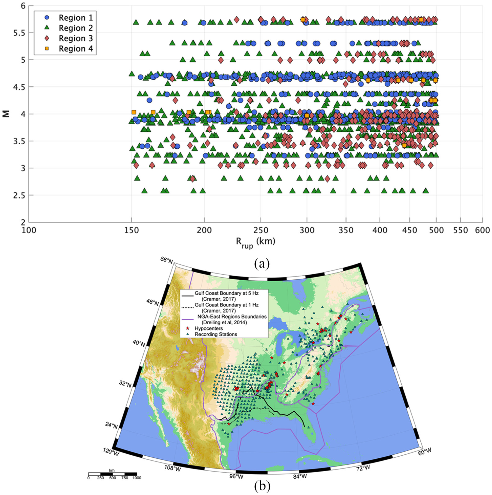
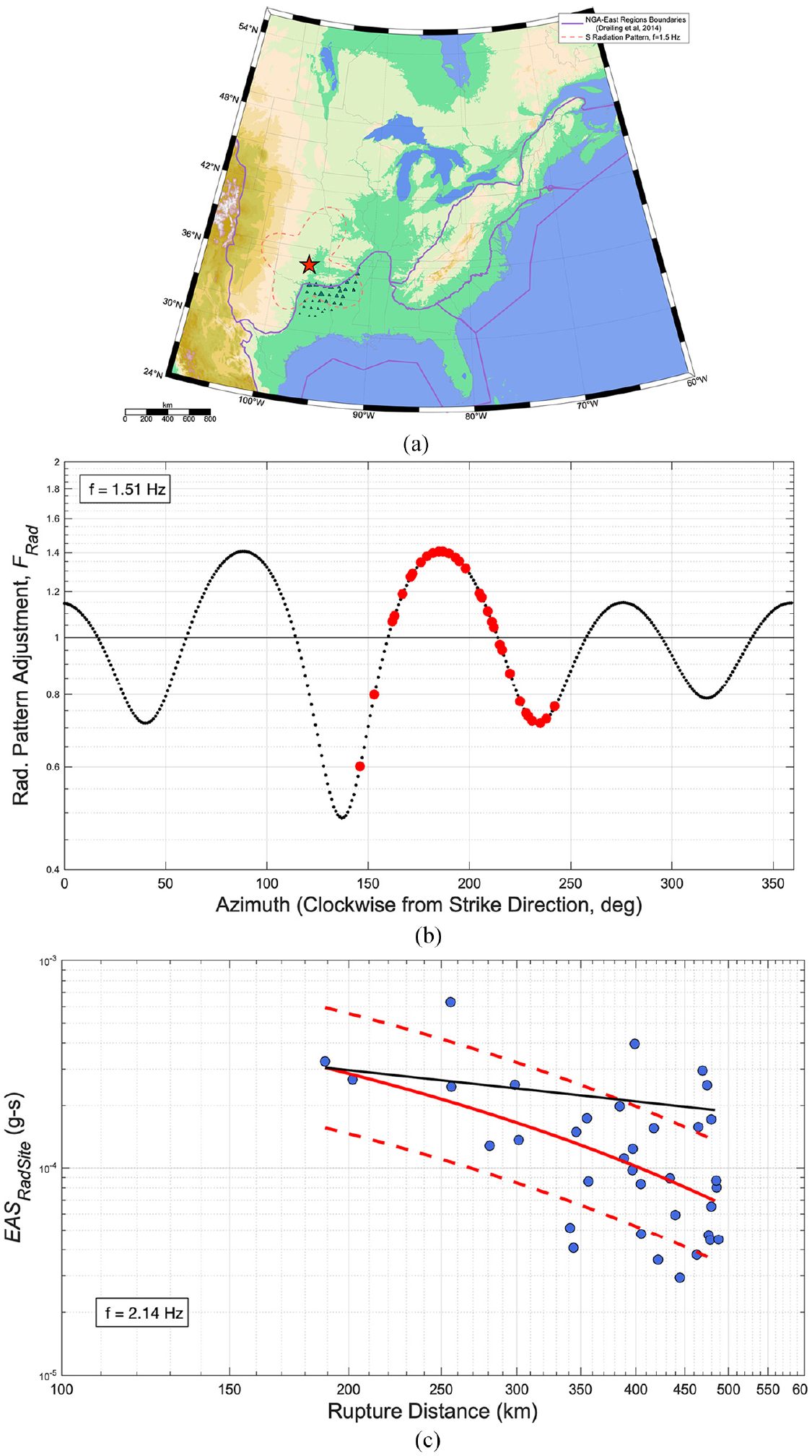
In addition to the quality assurance and review performed by PEER (2015), each $EAS$ is visually checked for outliers, poor quality data, or errors with units. After screening for data quality, recording distance, recording coverage, and frequency limitations, 53 earthquakes were identified as candidates for the analysis, each with at least five ground motion recordings. These earthquakes and their attributes are listed in Supplemental Table A-1 of Appendix A. Figure 2 shows a magnitude versus rupture distance scatter plot of this database at $f = 1$ Hz, and a map of these events along with the recording stations used in the analyses. This database encompasses over 2000 $EAS$ records from the 53 earthquakes. The regional $Q (f)$ estimates are derived from subsets of this database. Figure 2 shows the Dreiling et al. (2014) regionalization used for developing the regional apparent $Q (f)$ in this study, and for comparison, the Cramer (2017) Gulf Coast region boundaries at 1 and 5 Hz.

Figure 2.

Left: magnitude versus distance coverage of the data used in the $Q (f)$ analyses, at $f = 1$ Hz. Right: map of epicenters for the events used (red stars), along with all recording stations (green triangles) with data available at $f = 1$ Hz. The Dreiling et al. (2014) and Cramer (2017) region boundaries are given by the magenta and black lines, respectively.

Inversion for Q

Several studies (e.g. Chapman and Godbee, 2012; Frankel, 2015; Graves, 2013) have shown that radiation pattern and rupture directivity are important factors in determining the attenuation of ground motions (rate of decrease in ground motion amplitudes with distance), and that low-frequency amplitudes (in some cases up to 5 Hz) can be contaminated by radiation pattern and directivity effects. Consequently, it is preferable to take these factors into account when constructing GMPEs and $Q (f)$ models. The procedure taken to estimate the apparent $Q (f)$ for a given earthquake is as follows:

Gather the $EAS$ data and metadata. Filter by region as needed. The unmodified data are denoted as $EA S_{raw}$ ;

Calculate the site response adjustment for each record, $F_{Site}$ , as described below;

Calculate the radiation pattern effect adjustment for each record, $F_{Rad}$ , as described below;

Adjust the $EA S_{raw}$ for site effects (to obtain $EA S_{Site} = EA S_{raw} / F_{Site}$ ), for radiation pattern effects (to obtain $EA S_{Rad} = EA S_{raw} / F_{Rad}$ ), and for both effects to obtain $EA S_{RadSite} = EA S_{raw} / (F_{Site} F_{Rad})$ ;

Follow the Cramer (2017) procedure for estimating apparent $Q (f)$ . Assuming $1 / \sqrt{R}$ geometrical spreading, fit the attenuation of the $EAS$ at frequency $f$ to equation 5,

\begin{matrix} \ln [EAS (f)] = A (f) + b \ln [R_{rup}] + c (f) R_{rup} \end{matrix}

Equation 5

where $A (f)$ is a regression constant, $b = - 0.5$ , $R_{rup}$ is the closest distance to the rupture, and $c (f)$ is the apparent anelastic attenuation coefficient;

6. Estimate the apparent $Q (f)$ from $c (f)$ by equation 6.

\begin{matrix} Q (f) = \frac{- π f}{c (f) β_{0}} \end{matrix}

Equation 6

where $β_{0}$ is estimated for each event by interpolating the CENA 1D crustal model from Darragh et al. (2015) Table 3.2 for the shear wave velocity at the hypocentral depth. As in Atkinson and Boore (2014), the constraint that $c (f)$ must be negative is imposed; this corresponds to downward curvature of the attenuation of ground motions with distance. In cases where the range of mean $c (f)$ plus and minus one standard error ( $se$ ) contained positive estimates (corresponding to flat, or upward curvature of attenuation), this frequency was excluded from subsequent analyses.

This process is repeated for each earthquake in the dataset for 10 log-spaced frequencies ranging from to 1 to 20 Hz, and for each of $EA S_{raw}$ , $EA S_{Site}$ , $EA S_{Rad}$ , and $EA S_{RadSite}$ . These four variations of the ground motions are analyzed to assess the effectiveness of the site and radiation pattern corrections on apparent $Q (f)$ estimates. This effectiveness is quantified through analysis of the residual standard deviations ( $σ_{Resid}$ ) and the standard error of the $c$ coefficient estimates ( $s e_{c}$ ) in the “Results” section.

The frequency dependence of $Q (f)$ is then fit to the form $Q (f) = Q_{0} f^{η}$ . Both this fit and the fit in equation 5 are performed using an iteratively reweighted least-squares regression with Huber weighting and outlier detection (Holland and Welsch, 1977). In Huber weighting, observations with small residuals get a weight of one and observations with larger residuals are assigned reduced weights, and the estimating equation is solved iteratively for the coefficients until convergence. The apparent $Q (f)$ estimates using this procedure are whole record estimates, which at regional distances from shallow events are dominated by the $L_{g}$ phase (mixed with other phases), primarily composed of $S$ waves trapped within the lower seismic velocities in the crust (Kennett, 1986). Therefore, the results presented here are compatible with other studies to determine the frequency-dependent $L_{g}$ attenuation in CENA.

Site response

For the site response adjustment (Inversion Step 2), three existing linear models are considered. The first is the Harmon et al. (2019) linear model, which is developed specifically for smoothed $FAS$ in CENA. This model was developed from a parametric study of 1D ground response analyses of input rock motions propagated through soil columns representative of CENA site conditions using the software DEEPSOIL V6.1 (Hashash et al., 2016). The Harmon et al. (2019) linear $FAS$ model is in the form of tabulated ln(amplification) for a set of $V_{s 30}$ , ranging from 90 to 3000 m/s, and $f$ , ranging from 1 to 100 Hz. Interpolation is performed of the ln(amplification) for the $V_{s 30}$ of the site and for the frequency under consideration.

The second model considered is from Stewart et al. (2017), which as part of the NGA-East project, synthesized relevant research results to provide recommendations to the USGS for the modeling of ergodic site amplification in CENA for application in the next version of USGS maps. This panel recommended a model composed of three terms; the component used here is the linear site amplification term which describes $V_{s 30}$ scaling relative to a 760 m/s reference condition. This model is largely empirical, although it is designed for use with 5% damped pseudo-spectral acceleration instead of $FAS$ . Because this model is based on data in CENA, it is retained as one of the options. This model is applicable for $V_{s 30}$ from 200 to 2000 m/s and $f =$ 0.2 to 12.5 Hz.

The third model considered is from Bayless and Abrahamson (2019), which is an empirical $EAS$ ground motion model developed for California. One component of this ground motion model is an empirical, $V_{s 30}$ , and frequency-based linear site amplification term. This model is applicable for $V_{s 30}$ from 180 to 1500 m/s and $f =$ 0.1 to 24 Hz. The drawback of using this model is that it is derived from data recorded in California and Nevada, which is well known to have different geologic conditions than CENA. However, this model is also tested because it is designed for correcting the same intensity measure (smoothed $EAS$ ) as is used by PEER NGA-East and in this study.

The effectiveness of these models in estimating apparent $Q (f)$ is quantified through reductions in $σ_{Resid}$ and $s e_{c}$ relative to the uncorrected data, which imply that the attenuation of the data is fit better after applying the site correction. The comparison of $σ_{Resid}$ and $s e_{c}$ reductions for the three site response models is given in Supplemental Appendix C and is discussed in the “Results” section.

Radiation pattern

The radiation pattern adjustment (Inversion Step 3) is based on 2D estimations obtained by averaging the 3D radiation amplitude pattern focal sphere for S waves (equations 4.84 and 4.85 from Aki and Richards, 1980) over a narrow range of azimuths and take-off angles for a specific focal mechanism and source–receiver azimuth. The take-off angle is randomized around 30° (measured from horizontal) for high frequencies, where the randomization becomes narrower as the frequencies approach 1 Hz. Following Boore and Boatwright (1984), this take-off angle falls within the recommended range for regional source to site distances. Here S represents the total S motion $(= \sqrt{S H^{2} + S V^{2}})$ . For a given azimuth, the radiation coefficient is normalized by the average over the whole focal sphere. Using this procedure results in a dimensionless radiation amplitude pattern parameter that varies with azimuth, given the earthquake strike, rake, and dip. In most cases, the radiation pattern adjustment falls within a factor of 2.

The four-lobed apparent radiation pattern is expected to be gradually distorted with increasing frequency (Takemura et al., 2016). To model the saturation of radiation pattern with increasing frequency, the procedure of Pitarka et al. (2000) is followed in which, at higher frequencies, the 2D radiation pattern is washed out and becomes a circle (independent of azimuth) at 3 Hz. The $σ_{Resid}$ and $s e_{c}$ reductions after accounting for site and radiation pattern effects are given in Supplemental Appendix C.

Example inversion

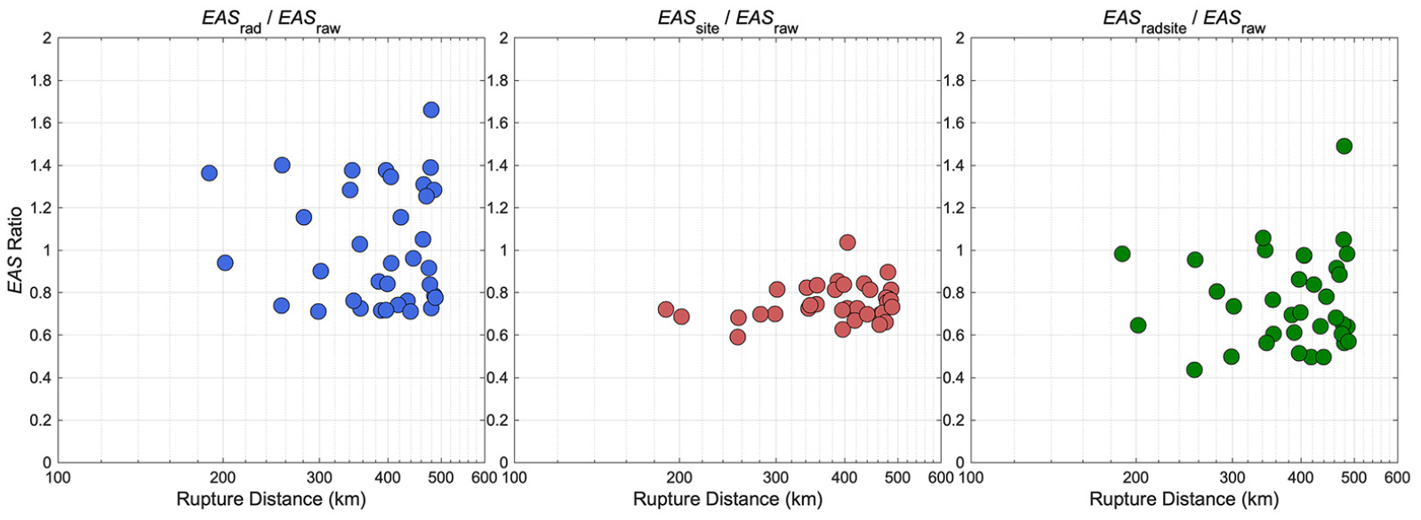
To illustrate this procedure, an example is given using data from the M4.7 Sparks earthquake (EQID 90) recorded in Region 1 (the Gulf Coast). Figure 3 shows a map of the earthquake epicenter and the recording stations used in this analysis. The 2D S-wave radiation pattern at $f = 1.5$ Hz for this earthquake is shown by the dashed line. At the same frequency, these data are processed as described previously (site effects based on frequency and $V_{s 30}$ , and radiation pattern effects based on the frequency and azimuthal variation of the 2D radiation pattern). The middle panel of Figure 3 shows these radiation pattern correction factors for $f = 1.5$ Hz versus azimuth, where the small black symbols are the 2D estimations of the total S-wave motion radiation amplitude pattern normalized by the average over the whole focal sphere, and the red circles are the recording stations. Figure 4 illustrates the effect each adjustment step has on the raw data in this example, at $f = 1.5$ Hz. In this example, the radiation pattern amplification ranges between 0.71 and 1.66, but the mean amplification over all sites is approximately unity because of the strong recording station azimuthal coverage of this earthquake (Figure 3). Because the $V_{s 30}$ of the sites in this example primarily lie in the range 400–600 m/s, the Stewart et al. (2017) site response adjustment reduces most of the EAS amplitudes at 1.5 Hz. The total adjustment for this example is shown in the rightmost panel of Figure 4.

Figure 3.

(a) a map showing the M4.7 Sparks earthquake epicenter (red star) and recording stations in Region 1 (green triangles) used in the inversion. The 2D S radiation pattern at $f = 1.5$ Hz is shown by the dashed line, for earthquake strike, rake, and dip of 300, 80, and −10°, respectively. (b) azimuthal variation of the radiation pattern adjustment, for the M4.7 Sparks earthquake. The small black symbols are the 2D estimations of the total S motion radiation amplitude pattern normalized by the averaged over the whole focal sphere. Red circles are the radiation pattern adjustment applied to the data at each station. (c) attenuation with distance at $f = 1.5$ Hz of the data ( $EA S_{RadSite}$ ), along with the mean fit of equation 10 (red), plus and minus one standard deviation. The black curve is the geometric spreading attenuation rate ( $b = - 0.5$ ) and $Q (f)$ models the departure from this rate.

Figure 4.

Ratios of the adjusted to non-adjusted EAS data versus distance after applying the radiation pattern adjustment (left), the site response adjustment (center) and both adjustments (right), for the M4.7 Sparks earthquake at $f = 1.5$ Hz.

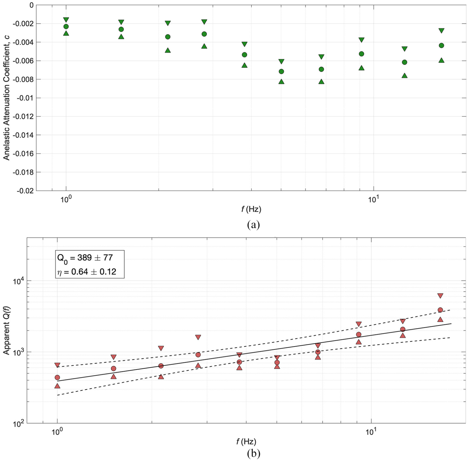
At each stage, the attenuation of the data is fit to equation 5, as shown in the bottom of Figure 3. This procedure is repeated for multiple frequencies to estimate the frequency dependence of the apparent anelastic attenuation, $c (f)$ , and the apparent $Q (f)$ on an event-by-event basis (e.g. Figure 4), and these results are combined to create the regional models.

The Sparks earthquake, shown in Figure 3, occurred within the CNA region but was well-recorded in the Gulf Coast region. Using this example, for the Gulf Coast region $Q (f)$ analysis, all of the available data within the Gulf Coast region were used (after applying the distance filter on the selection), regardless of the source-to-station travel distances through the CNA region. The Gulf Coast region analysis therefore includes some source-to-station paths with a significant amount of travel in the CNA region and some with considerably less. For a given distance, one might expect less attenuation of the ground motions at a station with most of the travel path in the CNA, compared to a station with most of the travel path in the Gulf Coast. This will contribute to increased scatter in the attenuation of the ground motions with distance (e.g. Figure 3) and would result in an increase in the standard error of the $c$ coefficient estimates ( $s e_{c}$ ). Any biases introduced by this effect (for all events) are not considered in the analysis and a more elegant treatment of the data selection is an area for future improvement.

Results

Within each region, apparent $Q (f)$ is estimated independently for each event. Results formatted similarly to Figures 3 and 5 are provided in Supplemental Appendix B for each of the four regions analyzed and for each event. Supplemental Appendix B also includes tables summarizing the estimated $Q (f)$ parameters and their uncertainties for each event.

Figure 5.

Results from the M4.7 Sparks earthquake (EQID 90) with data recorded in Region 1. Top: the mean apparent anelastic attenuation coefficient, $c$ (filled circles), versus frequency, with standard error of the coefficient (triangles). Bottom: the apparent $Q (f)$ . The mean (filled circles) and standard error (triangles) are given along with the mean fit (solid line) and 95% confidence intervals for the mean fit (dashed lines). $Q_{0}$ and $η$ with their standard errors are given in the figure.

As described previously, the inversion procedure is also performed on each of $EA S_{raw}$ , $EA S_{Site}$ , $EA S_{Rad}$ , and $EA S_{RadSite}$ to assess the effectiveness of these data corrections on modeling apparent $Q (f)$ . In addition, the procedure is repeated for each of the three alternative linear site amplification models. The final data correction method selection is based on the reductions in $σ_{Resid}$ and $s e_{c}$ relative to the uncorrected data. Supplemental Appendix C shows these reductions, both event-based and averaged over all events within a region, for each site amplification model and NGA-East region. Based on this assessment, the radiation pattern and site adjusted ground motions ( $EA S_{RadSite}$ ) are best fit to equation 5 when using the Stewart et al. (2017) site amplification model in the Gulf Coast and Appalachian regions, and using the Harmon et al. (2019) model in the CNA region. Therefore, these two site response models are adopted for these corresponding regions for the remainder of this study.

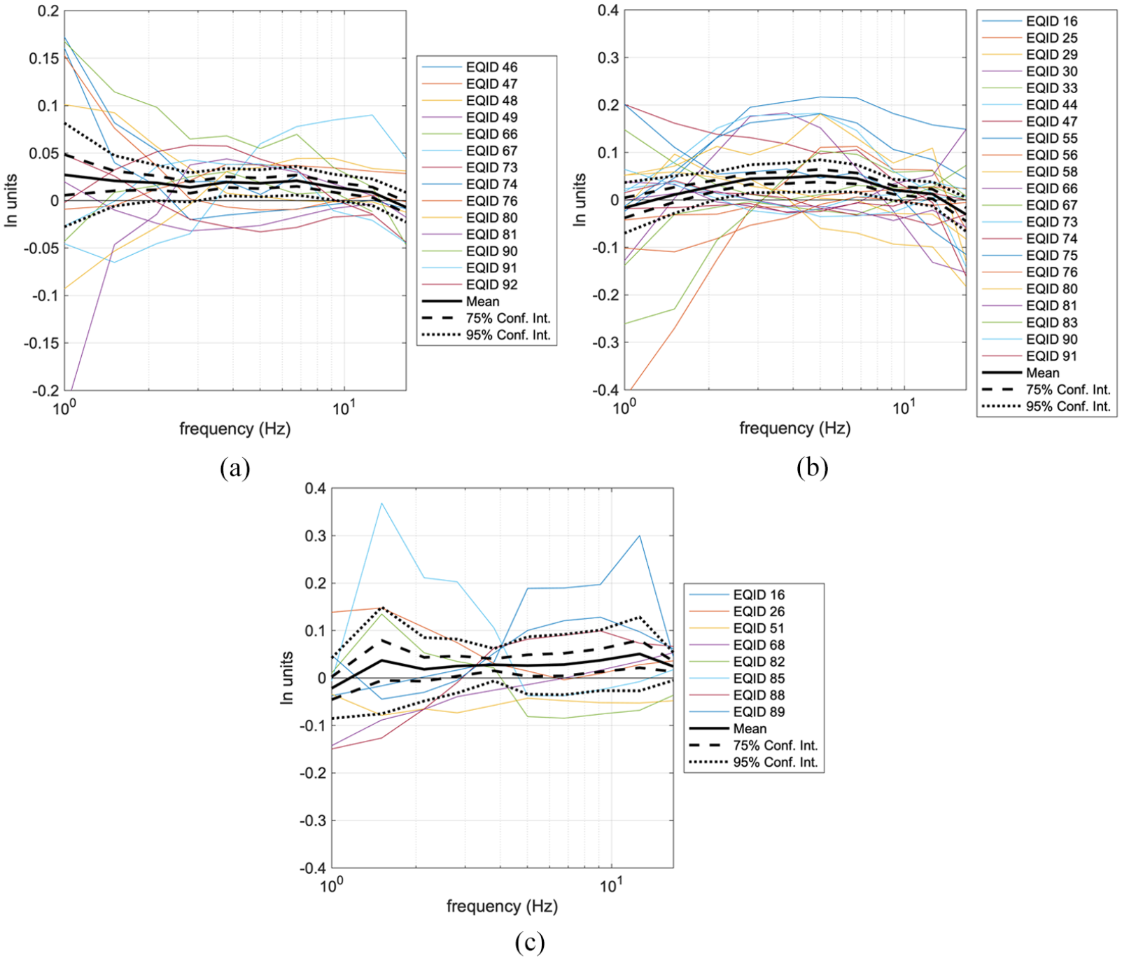
The difference in the $σ_{Resid}$ (natural log units) between $EA S_{raw}$ and $EA S_{RadSite}$ is shown for the three regions in Figure 6. Positive values represent a reduction in the standard deviation of residuals and improvement in the fit of the data to equation 5. Thin colored lines in Figure 6 are $σ_{Resid}$ differences for individual events, with some instances of improvement in the fit, and some instances of deterioration. The solid black line is the mean difference for all events, and the dashed and dotted black lines are the 75% and 95% confidence intervals about this mean, respectively. Where these confidence intervals do not cross below the zero line, the null hypothesis that the mean reduction of $σ_{Resid}$ is less than zero can be rejected with 75% and 95% confidence.

Figure 6.

The difference in the $σ_{Resid}$ (natural log units) between $EA S_{raw}$ and $EA S_{RadSite}$ versus frequency for (a) the Gulf Coast region, (b) the CNA region, and (c) the Appalachian Range region. Thin colored lines are $σ_{Resid}$ differences for individual events, the solid black line is the mean difference for all events, and the dashed and dotted black lines are the 75% and 95% confidence intervals about this mean.

Figure 6 shows that the reductions in $σ_{Resid}$ after applying the site response and radiation pattern adjustments are marginal. The reduction in total $σ_{Resid}$ ranges from 0% to 15% depending on the frequency. In addition, the radiation pattern adjustment has generally weaker influence on improving the attenuation modeling than the site response adjustment. The radiation pattern adjustment also has large variability in its effectiveness, as manifested by occurrences of increases in $σ_{Resid}$ for some events and decreases in others. This indicates that the simple algorithm used for the radiation pattern effect is too generic and is a matter with room for improvement in future studies. In the remainder of this study, the data corrected for site response and radiation pattern ( $EA S_{RadSite}$ ) are used because at most frequencies, there is a small, but statistically significant improvement (with 75% confidence) in the fit to equation 5 over the unadjusted data.

Regional models

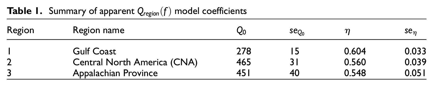
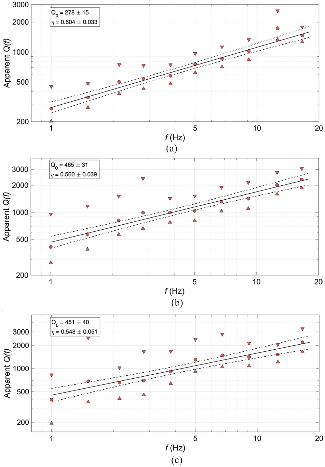
To develop a model for each region, the mean of the event-based estimates of apparent $Q (f)$ within each region is calculated. Figure 7 shows the mean $Q (f)$ (circles) with standard deviations (triangles) for the three regions. The best fit of the mean to the form $Q_{region} (f) = Q_{0} f^{η}$ is also shown with 95% confidence intervals (dashed lines). The regional model coefficients from this fit are listed in Table 1, along with their standard errors.

Table 1.

Summary of apparent $Q_{region} (f)$ model coefficients

Region	Region name	$Q_{0}$	$s e_{Q_{0}}$	$η$	$s e_{η}$
1	Gulf Coast	278	15	0.604	0.033
2	Central North America (CNA)	465	31	0.560	0.039
3	Appalachian Province	451	40	0.548	0.051

Figure 7.

Results for (a) the Gulf Coast, (b) the CNA, and (c) the Appalachian Province showing the $\bar{Q} (f)$ (filled circles) and standard deviations (triangles) of the event-based results. The mean fit (solid line) with 95% confidence intervals (dashed lines) is shown. Values of $Q_{0}$ and $η$ are given in each panel.

Discussion

There is general agreement that tectonically stable regions are usually described by higher $Q (f)$ and weaker frequency dependence ( $η$ ), while active regions are typically characterized by lower $Q (f)$ and stronger frequency dependence (e.g. Baqer and Mitchell, 1998; Cramer and Al Noman, 2016; Dreiling et al., 2014). Baqer and Mitchell (1998) attributed these differences to the greater amounts of interstitial crustal fluids in western North America. Furthermore, Baqer and Mitchell (1998) found the lowest $Q_{0}$ in the western United States, with intermediate values in the area spanning from the Colorado Plateau to the Rocky Mountains and in the southern Portion of the Atlantic Coastal Plain and the Gulf Coast, with the highest $Q_{0}$ in the Appalachians. These trends are generally consistent with the results given in Table 1. Based on the analysis, $Q_{0}$ is lowest in the Gulf Coast region ( $Q_{0} = 278 \pm 15$ ) and larger in the CNA region ( $Q_{0} = 465 \pm 31$ ) and the Appalachian Province ( $Q_{0} = 451 \pm 40) .$ The strongest frequency dependence is found in the Gulf Coast ( $η = 0.604 \pm 0.034$ ), and slightly lower frequency dependence is observed in the Appalachian Province ( $η = 0.548 \pm 0.051$ ) and CNA ( $η = 0.560 \pm 0.039$ ).

The $Q (f)$ models of Regions 2 (CNA) and 3 (Appalachian Province) are quite similar. Both parameters, $Q_{0}$ and $η$ , have mean values which are not statistically different from the other regions (Table 1). This suggests that these regions could be represented by the same effective anelastic attenuation. In the remainder of this article, I continue to treat these regions separately to compare with other regional models, but for practical purposes either model may be used (or the average of them) in either region. The lack of difference in $Q (f)$ between regions other than the Gulf Coast has previously been recognized by others, for example, Gupta et al., (1989), EPRI (1993), and Cramer (2017).

Model comparison

The models developed here are compared with a selection of published models for frequency-dependent Lg attenuation. Three Gulf Coast mean models are compared in Figure 8: Cramer and Al Noman (2016), Chapman and Conn (2016), and Silva et al. (2003). Several mean models for the CNA and ENA are given in Figure 9 because they are plentiful: Silva et al. (2002), Cramer and Al Noman (2016), Erickson et al. (2004), Atkinson and Boore (1995, 2014), Boatwright and Seekins (2011), and Atkinson (2004). Finally, five alternative mean models for the Appalachian region are compared against my model in Figure 10; Shi et al. (1996) and Erickson et al. (2004), plus three of the models used in the CNA comparison: Atkinson and Boore (1995, 2014), and Boatwright and Seekins (2011). Table 2 lists the models, and their associated parameters, which are compared in Figures 8 through 10. The geometric spreading coefficient ( $b$ value) is also given in Table 2 and in the figure legends.

Table 2.

$Q (f)$ models by others compared in Figures 8 through 10

Author	Region name	Applicable comparison region	$b$ ^a	$Q_{0}$	$s e_{Q_{0}}$	$η$	$s e_{η}$
Chapman and Conn (2016)	Gulf Coastal Plain of the Southern United States	1	−0.5	365	11.8	0.624	0.025
Cramer (2017), Cramer and Al Noman (2016)	Gulf Coast	1	−0.5	259	23	0.715	0.013
Silva et al. (2003)	Gulf Coast	1	−0.55^b	300	-	0.81	-
Cramer and Al Noman (2016)	Mid-Continent	2	−0.5	568	82	0.66	0.06
Silva et al. (2002)	Mid-Continent	2	−0.55^b	351	-	0.84	-
Erickson et al. (2004)	Central United States	2	−0.5	640	225	0.344	0.22
Atkinson and Boore (1995)	Eastern North America	2, 3	−0.5	680	-	0.36	-
Atkinson and Boore (2014)	Eastern North America	2, 3	−0.5	525	-	0.45	-
Boatwright and Seekins (2011)	Northeastern North America	2, 3	−0.5	410	25	0.5	0.03
Atkinson (2004)	Southeastern Canada and Northeastern United States	2	−0.5	1000^c	n/a	0.32	n/a
Shi et al. (1996)	Appalachian Province	3	n/a	574	12	0.46	0.05
Erickson et al. (2004)	Northeastern United States	3	−0.5	650	143	0.36	0.14

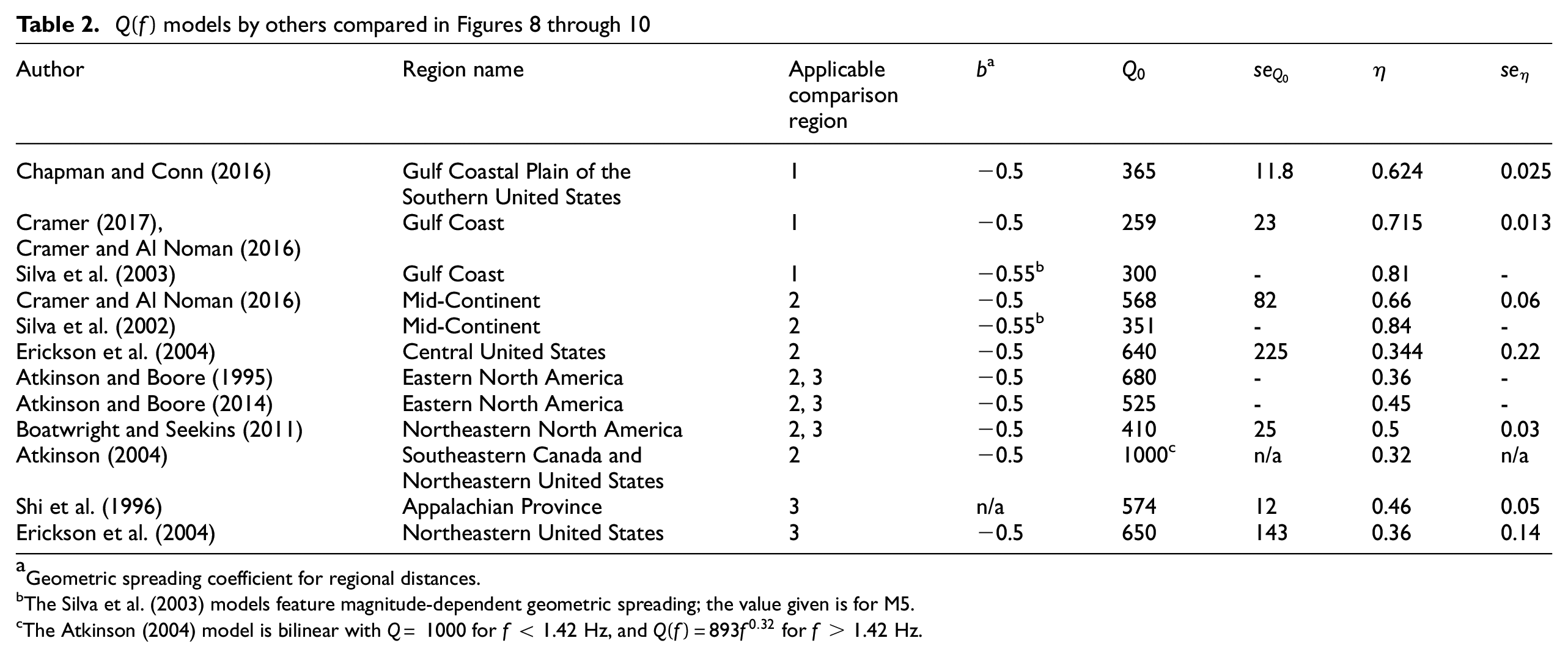
Geometric spreading coefficient for regional distances.

The Silva et al. (2003) models feature magnitude-dependent geometric spreading; the value given is for M5.

The Atkinson (2004) model is bilinear with $Q =$ 1000 for $f$ < 1.42 Hz, and $Q (f) = 893 f^{0.32}$ for $f$ > 1.42 Hz.

Figure 8.

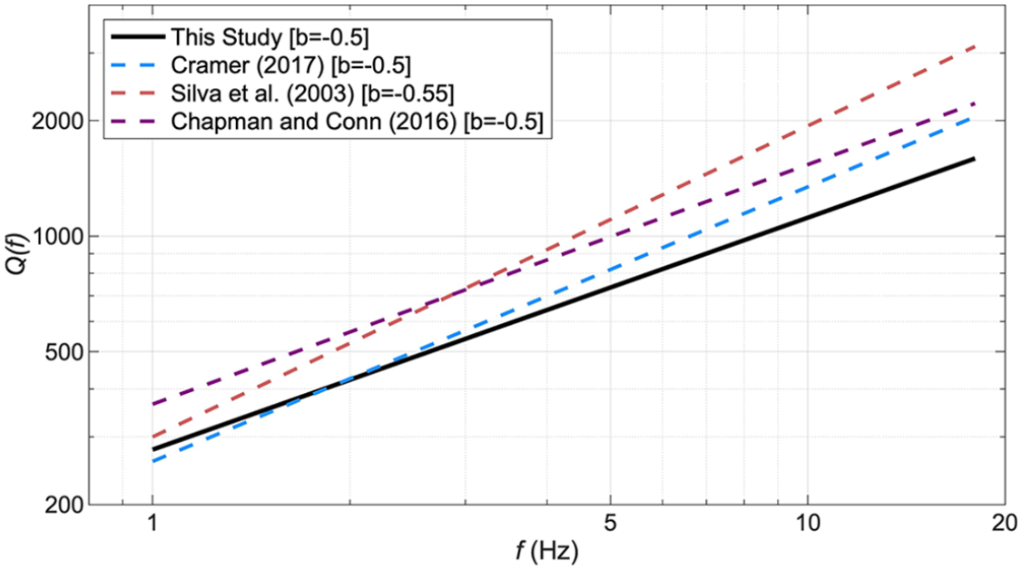
Comparison of mean $Q (f)$ models for the Gulf Coast region (Region 1).

Figure 9.

Comparison of mean $Q (f)$ models for the CNA or ENA regions with the Region 2 model.

Figure 10.

Comparison of mean $Q (f)$ models for the Appalachian Province region (Region 3).

The overlap of region definitions between previous studies complicates the apparent $Q (f)$ comparisons between models listed in Table 2. The CNA region used in this study (Region 2, as defined by PEER NGA-East; Dreiling et al., 2014) contains portions of the region others have described as the ENA, and the CNA region (Figure 1). For example, Atkinson and Boore (2014; their Figure 1) include the northeastern United States and southeastern Canada, but not CNA in their definition of ENA. In comparison, much of the Quebec region is included in the Dreiling et al. (2014) CNA region, but the region encompassed by Maine, New Brunswick, Nova Scotia, and Newfoundland is in the Appalachian Region. In the Gulf Coast, some (e.g. Cramer, 2017; Gallegos et al., 2014 implicitly) exclude the northern section of the Mississippi embayment in their regionalization, while others include it (e.g. Chapman and Conn, 2016; Dreiling et al., 2014). In light of these differences, the comparisons in Figures 8 through 10 are not one-to-one, but I have attempted to group the most appropriate models together based on their geographic regions; see column “Applicable Comparison Region” in Table 2.

Of the four mean Gulf Coast models compared in Figure 8, the one developed in this study has the mildest frequency dependence ( $η = 0.604 \pm 0.033$ compared with $η = 0.624 \pm 0.025, 0.715 \pm 0.013$ and $0.81$ ) and is within one standard error of the Chapman and Conn (2016) model. As discussed previously, the geometric spreading and anelastic attenuation terms can trade off with each other. The Silva et al. (2002) geometric spreading model is magnitude-dependent; the value shown ( $b = - 0.55$ ) corresponds to M5 and is therefore associated with a steeper geometrical attenuation than the one developed here. This leads to higher $Q (f)$ (lower damping) to counterbalance this attenuation. The current study value of $Q_{0} = 278 \pm 15$ lies in the range of the other three models and is within the standard error of both the Cramer (2017) and Silva et al. (2002) models. The differences in $η$ between the models leads to significant differences in $Q (f)$ at higher frequencies, as shown in Figure 8, where the current study mean $Q (f)$ is lower (higher damping) than all three mean models at frequencies greater than about 3 Hz. Cramer (2017) noted that the Chapman and Conn (2016) Gulf Coast region encompasses a larger mid-continental area than the Cramer (2017) region, which possibly explains the difference in $Q (f)$ between those models. The Chapman and Conn (2016) Gulf Coast region is similar to the Dreiling et al. (2014) regionalization, so that explanation does not apply to the differences observed from my model. The differences at high frequencies may be attributed to a combination of the ground motion database used and the site response adjustment applied to the data in the analysis.

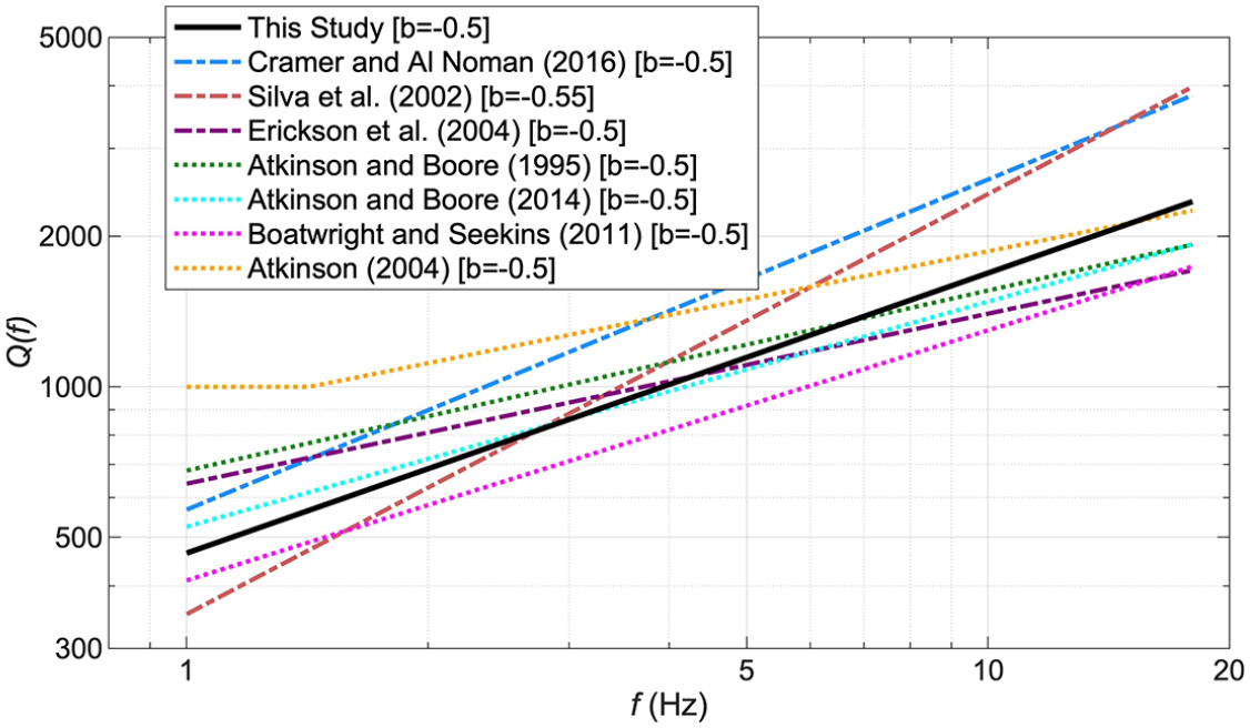
Figure 9 compares seven models developed for various named regions (Table 2) with the CNA region model from this study. This comparison is subject to the shortcomings previously mentioned, namely that they are for varying geographic regions. The first three (Cramer and Al Noman, 2016; Erickson et al., 2004; Silva et al., 2002) are models for the mid-continental and central United States (dashed lines). Similarly, the last four (Atkinson, 2004; Atkinson and Boore, 1995, 2014; Boatwright and Seekins, 2011) are models for what can grossly be called northeastern North America (dotted lines). The Dreiling et al. (2014) CNA region contains a large portion of the central United States and most of eastern Canada (Figure 1).

The current study value of $Q_{0} = 465 \pm 31$ is within the range of the seven other models, with the Boatwright and Seekins (2011; $Q_{0} = 410 \pm 25$ ) and Silva et al. (2002; $Q_{0} = 351$ ) having smaller $Q_{0}$ and the remaining five models having larger $Q_{0}$ . As with Silva et al. (2003), the Silva et al. (2002) geometric spreading model is magnitude-dependent and is associated with a steeper geometrical attenuation that has higher $Q (f)$ to counterbalance this. The slope parameter $η = 0.560 \pm 0.039$ from this study lies within the range of other models. The Atkinson (2004) model is the only model compared in Figures 8 through 10 which does not use the $Q (f) = Q_{0} f^{η}$ formulation; instead, this model is linear for frequencies greater than 1.42 Hz, and constant $Q (f) = 1000$ for frequencies less than 1.42 Hz.

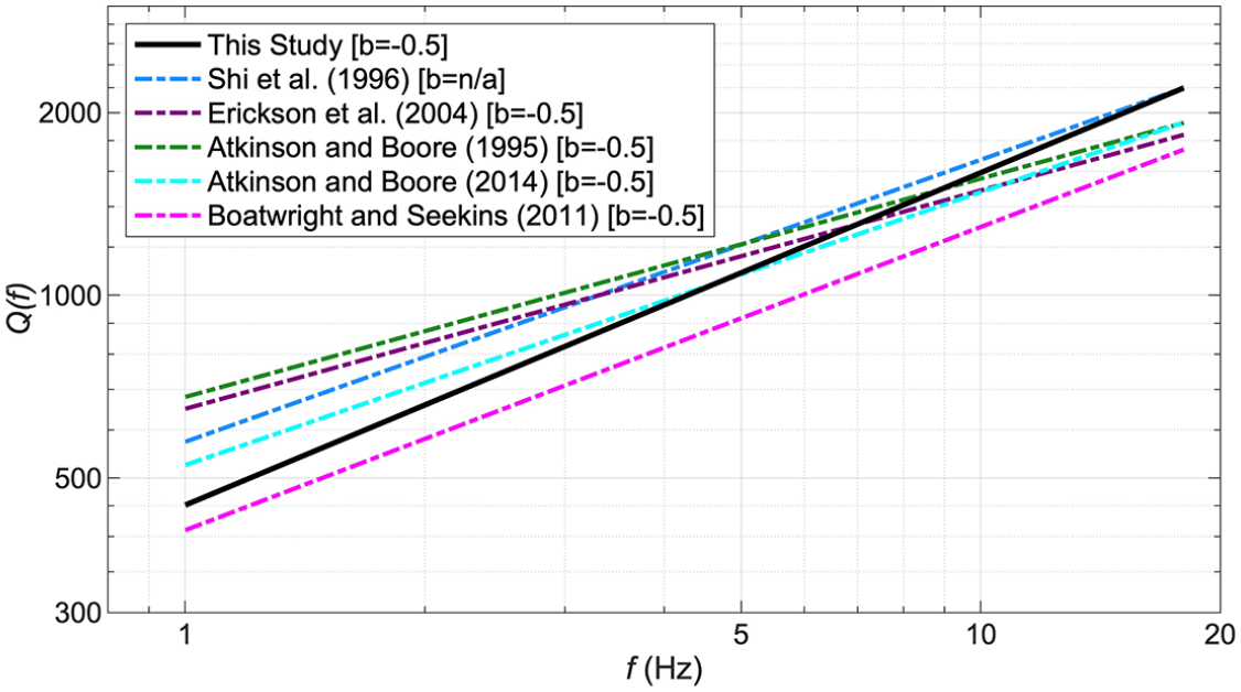
Figure 10 compares five models developed for various named regions (Table 2) with the Appalachian Province region model from this study. Three of these models (Atkinson and Boore, 1995, 2014; Boatwright and Seekins, 2011) are for what I call northeastern North America and were used in the CNA region comparison (Figure 9) but are relevant to this comparison as well because the Dreiling et al. (2014) Appalachian region extends to the north past Maine and includes Nova Scotia (Figure 1). The Shi et al. (1996) and Erickson et al. (2004) models are also developed for regions corresponding to the Dreiling et al. (2014) Appalachian Province. The current model ( $Q_{0} = 451 \pm 40, η = 0.548 \pm 0.051$ ) has steeper slope than each of these five models and lower $Q_{0}$ than four of them. The lower $Q_{0}$ and steeper slope result in similarity to the Shi et al. (1996) model at frequencies above about 10 Hz. The Shi et al. (1996) model does not assume any specific geometric spreading function because their $Q (f)$ is determined by fitting the spectral shape of $L_{g}$ wave displacement amplitude spectra (Shi et al. 1996). In general, the proposed $Q (f)$ model is lower at low frequencies than four of the other models and is higher than Boatwright and Seekins (2011) at all frequencies.

Evidence for other forms of $Q (f)$

There is an apparent “flattening” (as phrased here, in frequency space) between approximately 1–5 Hz in some of the event-based $Q (f)$ results from this study. This feature is not present in the $Q (f)$ of every event, nor is it present in the regional averages, but it is common enough in the event-based results to warrant discussion. These observations suggest that the linear form of $Q (f)$ may not be the most appropriate in all situations. Atkinson (2004) proposed a polynomial form for $Q (f)$ in the ENA to accommodate her observation that $Q (f)$ reached a minimum at 1 Hz and increased for lower and higher frequencies. Later, in Atkinson (2012), she found that an exponential form is preferable for $f > 1$ Hz because it is more stable at high frequencies. The flattening is also evident in results from other studies, as described below, but is not often discussed or modeled, presumably because the form $Q (f) = Q_{0} f^{η}$ has become standard due to its wide application and because there is no theoretical basis for a more complex model. Notable modeling exceptions are David Boore’s stochastic model (Boore, 2003) which allows for a trilinear $Q$ versus $f$ model, and Atkinson (2004) who proposed a polynomial model to accommodate the observation that $Q$ was at a minimum near 1 Hz and increased at both lower and higher frequencies.

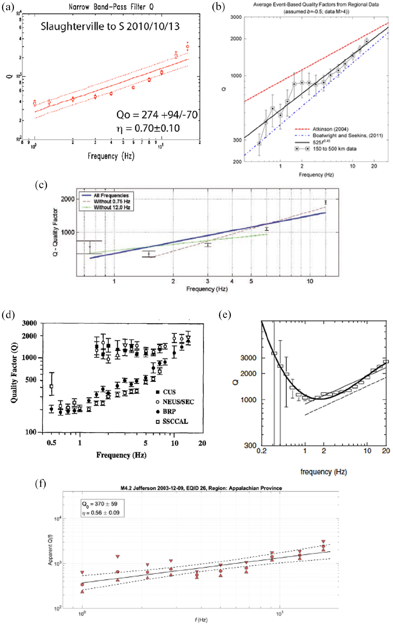
Figure 11 presents a few examples of this behavior of other empirical $Q (f)$ studies in different regions. All of these examples show some degree of a flat trend in the data points used to fit the models for frequencies from about 1.5 to 4 Hz. It could be argued that these would be better fit with bilinear, trilinear, or polynomial models. In Figure 11a, the Cramer and Al Noman (2016) result shows apparent $Q (f)$ in the Gulf Coast from the Slaughterville earthquake with a curvature in the data points that is similar to some of the results from this study. Figure 11b, from Atkinson and Boore (2014), shows multiple event-based apparent $Q (f)$ in ENA. In Figure 11c, from Erickson et al. (2004), the multiple event-based apparent $Q (f)$ in the central United States reaches a minimum value at 1.5 Hz and increases to the 3 Hz level at 0.75 Hz, which does not support a linear model well. Figure 11d replicates Figure 16 of Benz et al. (1997) which summarizes their Lg-based $Q (f)$ for four study regions; solid squares are the central United States and empty circles represent the northeastern United States and southeastern Canada. Both of these would be better fit with a bilinear model and than a linear one. Figure 11e, from Atkinson (2004), shows a polynomial fit to $Q (f)$ in ENA and is one of the few models identified which features increased $Q$ at the lowest frequencies. Finally, Figure 11f, from this study, shows apparent $Q (f)$ in the Appalachian Province from the Jefferson earthquake. The simple linear model is adopted in this study because it is not clear if this is a feature related to the anelastic attenuation or to source or site factors, but this interesting feature should be studied further.

Figure 11.

A collection of figures with results from other empirical $Q (f)$ studies. (a) Figure from Cramer and Al Noman (2016) showing apparent $Q (f)$ in the Gulf Coast from the Slaughterville earthquake. (b) Figure from Atkinson and Boore (2014) showing multiple event-based apparent $Q (f)$ in ENA. (c) Figure from Erickson et al. (2004) showing multiple event-based apparent $Q (f)$ in the central United States. (d) Figure 16 from Benz et al. (1997) showing Lg $Q (f)$ for four study regions; solid squares are the Central United States. (e) Figure from Atkinson (2004) showing a polynomial fit to $Q (f)$ in ENA. (f) From this study, apparent $Q (f)$ in the Appalachian Province from the Jefferson earthquake.

Events with data in multiple regions

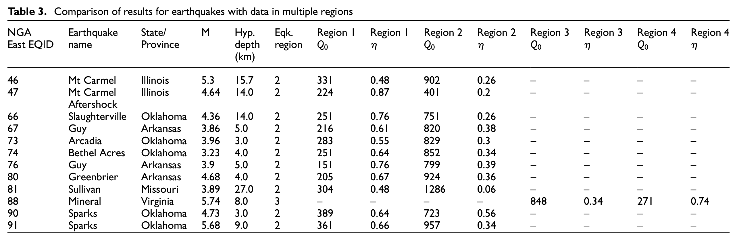
Table 3 lists the earthquakes analyzed that have data in multiple Dreiling et al. (2014) regions, along with the $Q_{0}$ and $η$ estimates for each. This comparison allows for testing the boundaries by identifying different apparent $Q (f)$ in multiple regions from the same earthquake. In total, 11 of these events have data in both Region 1 (Gulf Coast) and Region 2 (CNA). Qualitatively, the results are as expected and support the Dreiling et al. (2014) region boundaries because $Q_{0}$ is larger for the CNA data than for the Gulf Coast data, and $η$ values are smaller for the CNA as compared with the Gulf Coast. In fact, all 11 events have larger $Q_{0}$ for the CNA than for the Gulf Coast. Both the $Q_{0}$ and $η$ samples have statistically different means between Regions 1 and 2 at the 95% confidence level.

Table 3.

Comparison of results for earthquakes with data in multiple regions

NGAEast EQID	Earthquake name	State/Province	M	Hyp.depth (km)	Eqk. region	Region 1 $Q_{0}$	Region 1 $η$	Region 2 $Q_{0}$	Region 2 $η$	Region 3 $Q_{0}$	Region 3 $η$	Region 4 $Q_{0}$	Region 4 $η$
46	Mt Carmel	Illinois	5.3	15.7	2	331	0.48	902	0.26	–	–	–	–
47	Mt Carmel Aftershock	Illinois	4.64	14.0	2	224	0.87	401	0.2	–	–	–	–
66	Slaughterville	Oklahoma	4.36	14.0	2	251	0.76	751	0.26	–	–	–	–
67	Guy	Arkansas	3.86	5.0	2	216	0.61	820	0.38	–	–	–	–
73	Arcadia	Oklahoma	3.96	3.0	2	283	0.55	829	0.3	–	–	–	–
74	Bethel Acres	Oklahoma	3.23	4.0	2	251	0.64	852	0.34	–	–	–	–
76	Guy	Arkansas	3.9	5.0	2	151	0.76	799	0.39	–	–	–	–
80	Greenbrier	Arkansas	4.68	4.0	2	205	0.67	924	0.36	–	–	–	–
81	Sullivan	Missouri	3.89	27.0	2	304	0.48	1286	0.06	–	–	–	–
88	Mineral	Virginia	5.74	8.0	3	–	–	–	–	848	0.34	271	0.74
90	Sparks	Oklahoma	4.73	3.0	2	389	0.64	723	0.56	–	–	–	–
91	Sparks	Oklahoma	5.68	9.0	2	361	0.66	957	0.34	–	–	–	–

For comparing the other two regions, only the Mineral earthquake (EQID88) had data in both the Appalachian Province (Region 3) and in the Atlantic Coastal Plain (Region 4). The results for this single event are also consistent with Baqer and Mitchell (1998); the estimated $Q_{0}$ for the Appalachians ( $Q_{0} = 848, η = 0.34)$ is larger with less frequency dependence than for the Atlantic Coast ( $Q_{0} = 271, η = 0.74)$ .

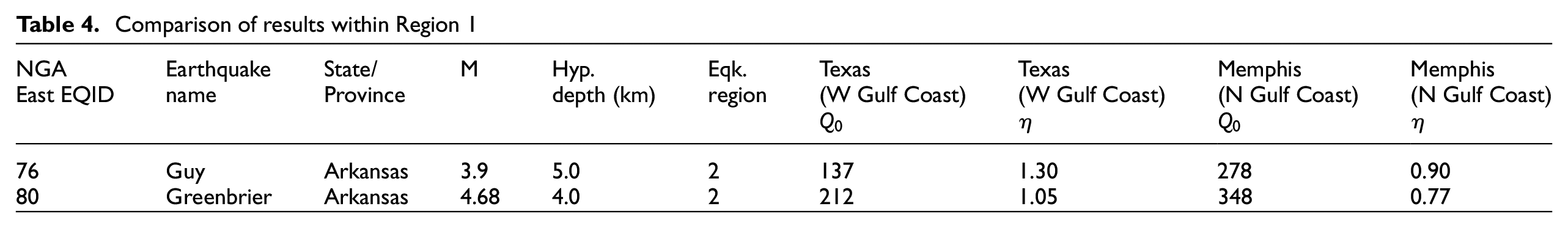
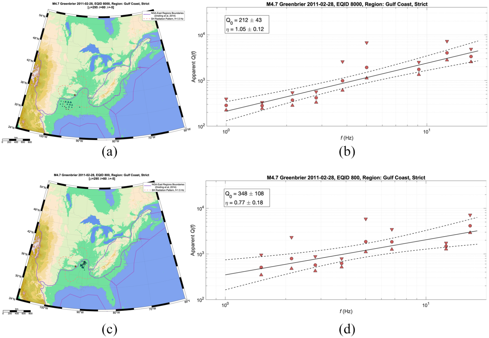
Two earthquakes are identified as good candidates for further testing of the sensitivity of apparent $Q (f)$ within the Dreiling et al. (2014) Gulf Coast region (Table 4). These are the Guy and Greenbrier earthquakes. Both events have enough data both in the northernmost section of the Dreiling et al. (2014) Gulf Coast region, which encompasses the Mississippi embayment and the region to the west (Texas area) that the analysis can be repeated for each sub-region separately. Figure 12 shows the division of the data and the results of this analysis for the M4.7 Greenbrier earthquake. Table 4 summarizes the event-based $Q (f)$ estimates for each sub-region. In both cases, the $Q_{0}$ estimate is larger and the $η$ estimate is smaller for the northern Mississippi embayment (Memphis region) compared with the Texas region. Cramer (2017) shows that the upper Mississippi embayment is outside the Gulf Coast region as far as attenuation is concerned; the Cramer (2017) region boundary is shown in Figure 2b. This result suggests that the Cramer (2017) Gulf Coast regionalization may be an improvement to the Dreiling et al. (2014) one. The refinement of this region with respect to attenuation models should be studied further. The conclusiveness of these results would benefit from more data than just two events.

Table 4.

Comparison of results within Region 1

NGAEast EQID	Earthquake name	State/Province	M	Hyp.depth (km)	Eqk. region	Texas (W Gulf Coast) $Q_{0}$	Texas (W Gulf Coast) $η$	Memphis (N Gulf Coast) $Q_{0}$	Memphis (N Gulf Coast) $η$
76	Guy	Arkansas	3.9	5.0	2	137	1.30	278	0.90
80	Greenbrier	Arkansas	4.68	4.0	2	212	1.05	348	0.77

Figure 12.

Comparison of results for the M4.7 Greenbrier earthquake in Region 1, split (a and b) to the southwest and (c and d) to the northeast.

Summary and conclusion

The goals of this article were to investigate and document differences in regional $Q (f)$ using the PEER NGA-East regionalization (Dreiling et al., 2014) and to provide regional $Q (f)$ models that can be used as epistemic alternatives to other existing models. This study uses smoothed $FAS$ data from well-recorded events in the CENA as collected and processed by PEER NGA-East (Goulet et al., 2014) and uses an assumption of average geometrical spreading applicable to the distance ranges considered, a correction for the radiation pattern effect, and a correction for site response based on $V_{s 30}$ . Independent analyses of the data are performed for the site response and radiation pattern effects and I find that together they slightly improve the estimates of $Q (f)$ , with the radiation pattern adjustment having generally weaker influence on the attenuation modeling than the site response. Apparent $Q (f)$ from multiple events is combined within each region to develop the regional models.

$Q (f)$ is usually modeled with the form $Q (f) = Q_{0} f^{η}$ , where $Q_{0}$ is the $Q$ value at 1 Hz, and $η$ is the slope parameter. Using this form, models are developed for three regions as defined by PEER (Dreiling et al., 2014): the Gulf Coast, CNA, and the Appalachian Province. Consideration of the $Q (f)$ model uncertainties suggests that the CNA and Appalachian Province regions could be combined. There was not sufficient data to adequately constrain the model for a fourth region, the Atlantic Coastal Plain. Significantly different regional $Q (f)$ is found for events with data recorded in multiple regions, which supports the NGA-East regionalization of the Gulf Coast and CNA. An inspection of two events recorded in the Dreiling et al. (2014) Gulf Coast region with data both in the northernmost Mississippi Embayment (Memphis region within the Dreiling et al., 2014 Gulf Coast region) and to the west (Texas area, within the Dreiling et al., 2014 Gulf Coast region) reveals higher $Q_{0}$ estimates in the Memphis region, indicating that the Cramer (2017) Gulf Coast regionalization may be an improvement to that of NGA-East for anelastic attenuation. This region is a candidate for potential refinement with respect to attenuation models in future investigations.

The regional models are consistent with expectations; the tectonically stable regions (CNA, Appalachian Province) are usually described by higher $Q (f)$ and weaker frequency dependence ( $η$ ), and the Gulf Coast model is characterized by lower $Q (f)$ and stronger frequency dependence. The $Q (f)$ models developed serve as epistemic uncertainty alternatives in CENA based on a literature review and a comparison with previously published models.

Supplemental Material

sj-pdf-1-eqs-10.1177_87552930211018704 – Supplemental material for Regional attenuation models in Central and Eastern North America using the NGA-East database

Supplemental material, sj-pdf-1-eqs-10.1177_87552930211018704 for Regional attenuation models in Central and Eastern North America using the NGA-East database by Jeff Bayless in Earthquake Spectra

Footnotes

Acknowledgements

This project was sponsored by the US Geological Survey (USGS) under award number G17AP00034. Thanks to the Pacific Earthquake Engineering Research Center for making their ground motion databases, including those from NGA-East, publicly available. Thanks to Christine Goulet for her assistance with the PEER NGA-East database and to Youssef Hashash and Okan Ilhan for providing guidance with their Fourier amplitude spectrum (FAS) site amplification model. Helpful review comments from David Boore, Chris Cramer, Paul Somerville, and one anonymous reviewer greatly improved the article. All maps in this report were created using the M_Map MATLAB package (Pawlowicz, 2019).

Data and resources

The ground motion data were processed by PEER NGA-East (Goulet et al., 2014) and provided by Christine Goulet (personal communication, 2019). Regression analyses and graphics production were performed using the numeric computing environment MATLAB (www.mathworks.com last accessed 17 Dec, 2020). MATLAB codes for our Q(f) inversion method are available at

Declaration of conflicting interests

The author(s) declared no potential conflicts of interest with respect to the research, authorship, and/or publication of this article.

Funding

This research was sponsored by the US Geological Survey (USGS) under award number G17AP00034.

Supplemental material

Supplemental material for this article is available online.

References

Abrahamson

Silva

(1997) Empirical response spectral attenuation relations for shallow crustal earthquakes. Seismological Research Letters 68(1): 94–127.

Abrahamson

Silva

(2001) “Empirical” attenuation relations for central and eastern U.S. hard and soft rock and deep soil site conditions. Seismological Research Letters 72: 282.

Aki

Richards

(1980) Quantitative Seismology. New York: Freeman.

Atkinson

(1984) Attenuation of strong ground motion in Canada from a random vibrations approach. Bulletin of the Seismological Society of America 74(6): 2629–2653.

Atkinson

(2004) Empirical attenuation of ground motion spectral amplitudes in southeastern Canada and the northeastern United States. Bulletin of the Seismological Society of America 94: 1079–1095.

Atkinson

(2012) Evaluation of attenuation models for the Northeastern United States/Southeastern Canada. Seismological Research Letters 83: 1166–1178.

Atkinson

Boore

(1995) Ground motion relations for eastern North America. Bulletin of the Seismological Society of America 85: 17–30.

Atkinson

Boore

(2014) The Attenuation of Fourier Amplitudes for Rock Sites in Eastern North America. Bulletin of the Seismological Society of America 104: 1513–1528.

Baqer

Mitchell

(1998) Regional variation of Lg Coda Q in the continental United States and its relation to crustal structure and evolution. Pure and Applied Geophysics 153: 613–638.

10.

Bayless

Abrahamson

(2019) Summary of the BA18 ground-motion model for Fourier amplitude spectra for crustal earthquakes in California. Bulletin of the Seismological Society of America 109: 2088–2105.

11.

Benz

Frankel

Boore

(1997) Regional Lg attenuation for the continental United States. Bulletin of the Seismological Society of America 87: 606–619.

12.

Bisrat

DeShon

Pesicek

Thurber

(2014) High-resolution 3-D P wave attenuation structure of the New Madrid Seismic Zone using local earthquake tomography, J. Geophys. Res. Solid Earth, 119, 409–424, https://doi.org/10.1002/2013JB010555

13.

Boatwright

Seekins

(2011) Regional spectral analysis of three moderate earthquakes in northeastern North America. Bulletin of the Seismological Society of America 101: 1769–1782.

14.

Boore

(1983) Stochastic simulation of high-frequency ground motions based on seismological models of the radiated spectra. Bulletin of the Seismological Society of America 73: 1865–1894.

15.

Boore

(2003) Simulation of ground motion using the stochastic method. Pure and Applied Geophysics 160: 635–676.

16.

Boore

(2005) Smsim-Fortran programs for simulating ground motions from earthquakes: Version 2.3-A Revision of OFR 96-80-A. U.S. Geological Survey Open-File Report.

17.

Boore

(2015) Point-source stochastic-method simulations of ground motions for the PEER NGA-East p0roject, chapter 2 in NGA-East: Median ground-motion models for the Central and Eastern North America Region. PEER Report 2015/04. Berkeley, CA: Pacific Earthquake Engineering Research Center, pp. 11–49.

18.

Boore

Atkinson

(1987) Stochastic prediction of ground motion and spectral response parameters at hard-rock sites in eastern North America. Bulletin of the Seismological Society of America 77(2): 440–467.

19.

Boore

Boatwright

(1984) Average body-wave radiation coefficients. Bulletin of the Seismological Society of America 74: 1615–1621.

20.

Brune

(1970) Tectonic stress and the spectra of seismic shear-waves from earthquakes. Journal of Geophysical Research 75: 4997–5009.

21.

Brune

(1971) Correction to “Tectonic stress and the spectra of seismic shear waves from earthquakes.” Journal of Geophysical Research 76: 5002.

22.

Burger

Somerville

Barker

Herrmann

Helmberger

(1987) The effect of crustal structure on strong ground motion attenuation relations in eastern North America. Bulletin of the Seismological Society of America 77: 420–439.

23.

Chapman

Conn

(2016) A Model for Lg propagation in the gulf coastal plain of the southern United States. Bulletin of the Seismological Society of America 106(2): 349–363.

24.

Chapman

Godbee

(2012) Modeling geometrical spreading and the relative amplitudes of vertical and horizontal high-frequency ground motions in Eastern North America. Bulletin of the Seismological Society of America 102: 1957–1975.

25.

Cramer

(2017) Gulf coast regional Q and boundaries from USArray data. Bulletin of the Seismological Society of America 108: 437–449.

26.

Cramer

Al Noman

(2016) Final technical report: Improving regional ground motion attenuation boundaries and models in the CEUS and developing a Gulf Coast empirical GMPE using EarthScope USArray data for use in the national seismic hazard mapping project. USGS grant G14AP00049, August 17, 52 pp.

27.

Dainty

(1981) A scattering model to explain seismic Q observations in the lithosphere between 1 and 20 Hz. Geophysical Research Letters 11: 1126–1128.

28.

Darragh

Abrahamson

Silva

Gregor

(2015) Development of hard rock ground-motion models for region 2 of Central and Eastern North America, chapter 3 in NGA-East: Median ground-motion models for the Central and Eastern North America Region. PEER Report 2015/04 (pp. 51–84). Berkeley, CA: Pacific Earthquake Engineering Research Center, University of California, Berkeley.

29.

Dreiling

Isken

Mooney

Chapman

Godbee

(2014) NGA-East regionalization report: Comparison of four crustal regions within Central and Eastern North America using waveform modeling and damped pseudo-spectral acceleration response. PEER Report No. 2014/15. Berkeley, CA: Pacific Earthquake Engineering Research Center, University of California, Berkeley.

30.

Electric Power Research Institute (EPRI) (1993) Guidelines for determining design basis ground motions. Volume 1. Method and guidelines for estimating earthquake ground motion in Eastern North America. Report EPRI TR-102293. Washington, DC: EPRI.

31.

Erickson

McNamara

Benz

(2004) Frequency dependent Lg Q within the continental United States. Bulletin of the Seismological Society of America 94(5): 1630–1643.

32.

Frankel

(2015) Decay of S-wave amplitudes with distance from earthquakes in the Charlevoix, Quebec area: Effects of radiation pattern and directivity. Bulletin of the Seismological Society of America 105(2a): 850–857.

33.

Gallegos

Ranasinghe

Sandvol

(2014) Lg attenuation in the central and eastern United States as revealed by the EarthScope transportable array. Earth and Planetary Science Letters 402: 187–196.

34.

Goulet

Bozorgnia

Abrahamson

(2015) Introduction to NGA-East: Median ground-motion models for the Central and Eastern North America Region. Chapter 1 of PEER Report 2015/04 (1–9). Berkeley, CA: Pacific Earthquake Engineering Research Center, University of California, Berkeley.

35.

Goulet

Kishida

Ancheta

Cramer

Darragh

Silva

Hashash

YMA

Harmon

Stewart

Wooddell

Youngs

(2014) PEER NGA-East database. PEER Report No. 2014/17, October. Berkeley, CA: Pacific Earthquake Engineering Research Center, University of California, Berkeley.

36.

Graves

(2013) Summary of geometrical spreading and Q models from recent events. In: 22nd international conference on structural mechanics in reactor technology (SMiRT-22) NGA-East special session, San Francisco, CA, 18–23 August.

37.

Guo

Chapman

(2019) An examination of amplification and attenuation effects in the Atlantic and Gulf Coastal Plain using spectral ratios. Bulletin of the Seismological Society of America 109(5): 1855–1877.

38.

Gupta

McLaughlin

Wagner

Jih

McElfresh

(1989) Seismic wave attenuation in Eastern North America. EPRI Rept. NP-6304, Palo Alto, CA: Electric Power Research Institute, 71 pp.

39.

Hanks

McGuire

(1981) The character of high-frequency strong ground motion. Bulletin of the Seismological Society of America 71: 2071–2095.

40.

Harmon

Hashash

Stewart

Rathje

Campbell

Silva

Ilhan

(2019) Site amplification functions for central and eastern North America–Part II: Modular simulation-based models. Earthquake Spectra 35(2): 815–847.

41.

Hashash

YMA

Musgrove

Harmon

Groholski

Phillips

Park

(2016) DEEPSOIL V6.1 (User Manual). Urbana, IL: University of Illinois at Urbana-Champaign, 137 pp.

42.

Holland

Welsch

(1977) Robust regression using iteratively reweighted least-squares. Communications in Statistics: Theory and Methods A6: 813–827.

43.

Hollenback

Kuehn

Goulet

Abrahamson

(2015) PEER NGA-east median ground motion models, chapter 11 in NGA-east: Median ground-motion models for the Central and Eastern North America Region. PEER Report 2015/04 (pp. 273–310). Berkeley, CA: Pacific Earthquake Engineering Research Center, University of California, Berkeley, CA.

44.

Kennett

(1986) Lg waves and structural boundaries. Bulletin of the Seismological Society of America 76(1): 133–1141.

45.

Konno

Ohmachi

(1998) Ground-motion characteristics estimated from spectral ratio between horizontal and vertical components of microtremor. Bulletin of the Seismological Society of America 88 (1): 228–241.

46.

Kottke

Rathje

Boore

Thompson

Hollenback

Kuehn

Goulet

Bozorgnia Abrahamson

Der Kiureghian

(2018). Selection of random vibration procedures for the NGA east project, PEER Report. No. 2018/05, Pacific Earthquake Engineering Research Center, University of California, Berkeley, California.

47.

Pasyanos

(2013) A lithospheric attenuation model for North America. Bulletin of the Seismological Society of America 103: 3321–3333.

48.

Pawlowicz

(2019) M_map: A Mapping Package for MATLAB, version 1.4K. Available at: www.eoas.ubc.ca/~rich/map.html (accessed May 19, 2021)

49.

PEER (2015) NGA-East: Median ground-motion models for the Central and Eastern North America region. PEER Report No. 2015/04, April. Berkeley, CA: University of California Berkeley.

50.

Pitarka

Somverille

Fukushima

Uetake

Irikura

(2000) Simulation of near-fault strong-ground motion. Bulletin of the Seismological Society of America 90(3): 566–586.

51.

Sandoval

Yassminh

(2014) Seismic attenuation and hazard in the Central and Eastern U.S. US Geological Survey report, G14AP00036.

52.

Shi

Kim

Richards

(1996) Variability of crustal attenuation in the Northeastern United States from Lg waves. Journal of Geophysical Research 101: B1125231–B1125242.

53.

Silva

Gregor

Darragh

(2002) Development of regional hard rock attenuation relations for central and eastern North America. Report prepared by Pacific Engineering and Analysis, El Cerrito, CA. Available at: http://www.pacificengineering.org/rpts_page1.shtml (accessed May 19, 2021)

54.

Silva

Gregor

Darragh

(2003) Development of regional hard rock attenuation relations for central and eastern North America, Mid-Continent, and Gulf Coast Areas. Report prepared by Pacific Engineering and Analysis, El Cerrito, CA. Available at: http://www.pacificengineering.org/gulf/Development%20ENA%20Midcontinent%20Gulf.pdf

55.

Somerville

McLaren

Saikia

Helmberger

(1990) The November 25, 1988 Saguenay, Quebec earthquake: Source parameters and the attenuation of strong ground motion. Bulletin of the Seismological Society of America 80: 1118–1143.

56.

Stewart

Parker

Harmon

Atkinson

Boore

Darragh

Silva

Hashash

YMA

(2017) Expert panel recommendations for ergodic site amplification in Central and Eastern North America. Report prepared for the Pacific Earthquake Engineering Research Center Report No. 2017/04. Berkeley, CA: University of California, Berkeley.

57.

Takemura

Kobayashi

Yoshimoto

(2016) Prediction of maximum P- and S-wave amplitude distributions incorporating frequency- and distance-dependent characteristics of the observed apparent radiation patterns. Earth, Planets and Space 68: 166.

58.

Toro

Abrahamson

Schneider

(1997) Model of strong ground motions from earthquakes in central and eastern North America: Best estimates and uncertainties. Seismological Research Letters 68: 41–57.

59.

Yassminh

Laphim

Sandvol

(2020) Seismic attenuation and velocity measurements of the uppermost mantle beneath the Central and Eastern United States and implications for the temperature of the North American lithosphere. Journal of Geophysical Research, Solid Earth, 125, e2019JB017728. https://doi.org/10.1029/2019JB017728

Regional attenuation models in Central and Eastern North America using the NGA-East database

Abstract

Keywords

Introduction

Previous work

Approach

Ground motion data

Data selection

Inversion for Q

Site response

Radiation pattern

Example inversion

Results

Regional models

Discussion

Model comparison

Evidence for other forms of Q ( f )

Events with data in multiple regions

Summary and conclusion

Supplemental Material

sj-pdf-1-eqs-10.1177_87552930211018704 – Supplemental material for Regional attenuation models in Central and Eastern North America using the NGA-East database

Footnotes

Acknowledgements

Data and resources

Declaration of conflicting interests

Funding

Supplemental material

References

Evidence for other forms of $Q (f)$