






Abstract
Maintaining the functionality of wastewater networks is critical to individual well-being, business continuity, public health, and safety. However, seismic damage and loss assessments of wastewater networks traditionally use fragility functions based on median repair rates without considering relevant sources of uncertainty and correlations of damage when estimating potential damage states and pipe repairs. This study presents a probabilistic methodology to incorporate modeling uncertainty (e.g. model parameter and model class uncertainty) and spatial correlations (e.g. spatial auto- and cross-correlation) of pipe repairs. The methodology was applied to a case study backbone system of a wastewater network in Portland, OR, using the expected hazard intensity maps for multiple deterministic earthquake scenarios, including a moment magnitude M6.8 Portland Hills Fault and M8.1, M8.4, M8.7, and M9.0 Cascadia Subduction Zone (CSZ) events. As spatial-correlation models of pipeline damage were non-existent in the literature and local information on costs to repair the pipes was limited at the time of this study, correlation methods and repair costs were proposed to estimate lower and upper bounds of pipe damage and loss. The results show how the consideration of different levels of uncertainty and spatial correlation for pipe repair rate could lead to different probabilistic estimates of damage and loss at the system level of the wastewater network, even though the point estimates, such as the mean and median, remain essentially unaltered.
Introduction
Maintaining the functionality of wastewater networks after earthquakes is critical to business continuity, public health, safety, and individual comfort. However, wastewater systems have experienced significant damage during past earthquakes, disrupting emergency response and delaying recovery efforts (Eidinger and Schiff, 1998; Nagata et al., 2011; Zare et al., 2011). Despite the direct and indirect consequences of losing the functionality of wastewater services, methods for the comprehensive probabilistic seismic damage and loss assessment of wastewater systems often do not consider all the relevant sources of uncertainty and correlation, even though well-established performance-based earthquake engineering methodologies (Federal Emergency Management Agency (FEMA), 2012; Moehle and Deierlein, 2004) incorporate uncertainty and correlation for other infrastructure and lifelines, such as for buildings and bridges.
Damage to wastewater networks has affected post-earthquake recovery in Japan and New Zealand. Wastewater treatment plants, lift stations, and pipelines were heavily damaged during the 1995 Kobe, Japan earthquake. The largest treatment plant was rebuilt over three years. Along the 3799-km long wastewater and stormwater pipelines, 1414 repairs were made to pipes damaged due to uplift or settlement of manholes, damage to road surfaces, or inflow and accumulation of soil in the pipes (Eidinger and Schiff, 1998). Following the 2004 Niigata earthquake in Japan, 9000 instances of pipe damage were observed along the 2672-km wastewater network, with over 1300 reported cases of manhole settlement or uplift (Scawthorn et al., 2006). After the 2010–2011 Canterbury, New Zealand earthquake sequence (CES), the Christchurch wastewater network was considered near failure. Wastewater treatment plants operated at 30% capacity, and the system leaked 40 million liters of wastewater per day into backyards and watercourses (Eidinger and Tang, 2011). As a result of the widespread liquefaction and lateral spreading during this event, observed damage to wastewater systems included pipe breakage in the form of loss of grade in gravity pipes causing partial or complete silt blockages, groundwater infiltration reducing the capacity of the pipes to carry wastewater, and differential settlement at manholes and pump stations. In addition, some pipe damage due to collocated asset failures was observed (Zorn and Shamseldin, 2017). Temporary facilities such as chemical and portable toilets were used for several months to relieve strain on the wastewater system (Kongar et al., 2017).
Despite the damage observed after past earthquakes, little effort has been made to collect the data necessary to develop empirical-based fragility models for wastewater pipelines (e.g. Baris et al., 2021; Liu et al., 2015; Nagata et al., 2011; Shoji et al., 2011). Moreover, little to no effort has been made to collect data to inform pipe damage correlation models for wastewater pipes (e.g. level of hazard and type of pipe with associated damage). In part, data collection has not been as rigorous for wastewater pipelines as for water pipelines, because, historically, there has been limited interest in the performance assessment of wastewater systems, and the majority of the damage in wastewater systems, especially minor leakage, has not been reported in the literature. Thus, empirical fragility functions have mostly focused on major damage to wastewater pipes (e.g. near complete blockage, loss of flow, or floatation). Knowledge of damage after an earthquake can also be limited based on what is known about the pipes before an event; for example, if a rigorous inspection program is not in place, it can be difficult to distinguish present or exacerbated damage from new damage due to the seismic event. In addition, several older localities do not have complete information about their infrastructure systems. As the inspection of large systems can take years, sometimes the damage is not easily “observable” for days to months.
Compared to the large body of literature related to the seismic assessment of other lifeline network systems, only a few of studies have assessed the seismic performance of wastewater systems; e.g., in contrast to potable water distribution systems (Cimellaro et al., 2016; Farahmandfar et al., 2017; Farahmandfar and Piratla, 2018; Fragiadakis and Christodoulou, 2014; Mazumder et al., 2020). Generally, existing studies on wastewater systems can be classified as: (1) reconnaissance studies reporting damage sustained to wastewater systems and the associated factors contributing to the vulnerability of the pipelines (Eidinger and Schiff, 1998; Eidinger and Tang, 2011; Giovinazzi et al., 2015; Scawthorn et al., 2006; Sherson et al., 2015; Zare et al., 2011), (2) empirical studies developing fragility functions for wastewater pipes based on reconnaissance observations (Baris et al., 2021; Liu et al., 2015; Nagata et al., 2011; Shoji et al., 2011), and (3) analytical studies evaluating the seismic performance of wastewater systems (Makhoul et al., 2020; Sigfúsdóttir, 2020; Sousa et al., 2012). Findings have included: (1) the predominant mode of failure is floatation of the pipes or manholes, due to differential settlements caused by liquefaction, (2) pipe failure decreases with increasing diameter and burial depth, and (3) some pipe materials, such as asbestos cement (AC), unreinforced concrete (CONC), cast iron (CI), earthenware (EW), and reinforced concrete with rubber rings (RCRRs), are inherently more vulnerable than other pipe materials, such as polyethylene (PE), polyvinylchloride (PVC), or high-density polyethylene (HDPE) (Giovinazzi et al., 2015).
Although these studies have highlighted the potential vulnerability of wastewater networks to seismic damage, fragility functions for wastewater pipelines are only available for a limited number of pipe types and material categories. Thus, common practice uses fragility functions developed for potable water pipes to estimate the vulnerability of wastewater pipes (e.g. American Lifelines Alliance (ALA), 2001; FEMA, 2010; Makhoul et al., 2020; SYNER-G, 2013). Similar practices have also been used to assess the vulnerability of other lifeline network systems, for example, natural gas systems (e.g. Jahangiri and Shakib, 2018; Kwong et al., 2022; Tsinidis et al., 2019). However, such practices can underestimate the physical damage to wastewater gravity pipelines, as observed after past earthquakes (Liu et al., 2015), due to: (1) differences in modeling the fluid flow in the different pipe systems (e.g. pressurized flow in water and natural gas systems vs predominantly gravity flow in wastewater systems) and (2) use of unique materials in wastewater systems, such as vitrified clay pipe (VCP), terra cotta pipe (TCP), and corrugated metal pipe (CMP). More recently, fragility functions have been developed in terms of damage ratios per unit length, such as the number of faults per km, to account for materials unique to wastewater systems (e.g. for Hume, VU, VP, PVC, and tile pipes (Shoji et al., 2011) and AC, CI, CONC, EW, RCRR, PVC, and PE pipes (Liu et al., 2015; Nagata et al., 2011)), functional disruption length per km (Shoji et al., 2011), and repair rate, defined as the number of repairs per km, with respect to peak ground velocity (PGV) or liquefaction potential index (LPI) (Baris et al., 2021).
Furthermore, although ALA (2001) fragility functions, which are considered the industry standard for assessing the seismic vulnerability of pipelines, provide variability of pipe fragility in terms of lognormal standard deviations, fragility functions based on median repair rates are widely used for the seismic assessment of pipelines in practice, by industry and research communities alike (Makhoul et al., 2020; Sigfúsdóttir, 2020). However, the use of median repair rate fragility functions does not account for the variability in damage to wastewater pipelines observed after seismic events. The variability in pipe vulnerability suggested in ALA (2001) assumes uniform seismic performance for all pipes irrespective of material, geometry, and physical condition. In contrast, Sousa et al. (2012) noted the importance of considering variability in the vulnerability of buried pipes based on their physical condition, which can vary significantly within a network, and proposed a method to characterize variabilities in pipe repair rates as a function of the structural condition of the pipes, ranging from very poor to excellent.
Using median fragility functions may neglect important sources of variability in estimates of wastewater pipe damage and repair, especially since several sources of uncertainty are known to be important for reliable seismic risk and loss assessment of other infrastructure systems, including model parameter uncertainty (Dolsek, 2009; Gokkaya et al., 2016; Liel et al., 2009) and model class uncertainty ( Alam, 2019; Alam and Barbosa, 2018; Barbosa, 2011; Muto and Beck, 2008; Romano et al., 2021). Model parameter uncertainty relates to the definition of the idealized parameters used in the model to simulate actual behavior, which can increase dispersion in the simulated response and, if neglected, can result in unconservative estimates (Liel et al., 2009). Model class uncertainty relates to the selection of one or multiple models from an appropriate class of models to describe a physical phenomenon. Estimates of median seismic demands using different model classes can differ significantly (Alam and Barbosa, 2018). Although the use of multiple models is common practice for probabilistic seismic hazard analysis (PSHA), its application to the seismic damage and loss assessment of lifeline and civil infrastructure is relatively new. To date, seismic damage and resilience assessments of wastewater networks have relied on fragility functions based on median repair rates (Makhoul et al., 2020; Sigfúsdóttir, 2020) without considering uncertainty in the fragility function due to model parameter or model class uncertainty.
In addition, spatial correlations of pipe damage are often neglected when assessing wastewater networks, even though wastewater pipes are spatially distributed over large areas. Excitation due to infrequent but strong seismic events can simultaneously excite spatially distributed infrastructure in a region (such as buildings, roads and bridges, and water and wastewater pipelines). As a result, there is an increased likelihood of simultaneous response of distributed infrastructure during strong ground shaking. Spatial correlation can be due to correlations in the ground motion intensity measure (IM) (e.g. Du and Wang, 2013; Goda and Atkinson, 2010; Goda and Hong, 2008b; Jayaram and Baker, 2009; Loth and Baker, 2013; Sokolov et al., 2010) or correlations in response and damage (e.g. DeBock et al., 2014; Goda and Hong, 2008a). The spatial correlation of infrastructure response is partly due to the spatial correlation of ground motion IMs arising from similarities in wave propagation path (path effects) and local site effects (similar terrain or soil conditions) and partly due to similarities in design and quality of construction of the infrastructure in a particular region, among many other factors (Shome et al., 2012). Generally, this spatial correlation decreases with increasing distance between two sites and can significantly vary depending on the earthquake record (Jayaram and Baker, 2009). Existing spatial-correlation models have considered the correlation between seismic damage and loss of distributed infrastructure in terms of different ground motion parameters, including peak ground acceleration (PGA), PGV, spectral acceleration
Incorporating spatial correlation in the assessment of wastewater systems is additionally hampered by the lack of spatial-correlation models for permanent ground deformation (PGD), which is widely used to model the fragility of pipelines under liquefaction and landslide-induced lateral spreading and ground settlement. Neglecting potential spatial correlation between damage of two different infrastructure components can overestimate or underestimate loss for frequent and rare earthquakes, respectively (Bazzurro et al., 2008; Goda and Hong, 2008a; Weatherill et al., 2015). For example, correlations were found to be significant between building engineering demand parameters (EDPs) for a portfolio of buildings in Los Angeles with similar fundamental periods located at closely spaced sites (DeBock et al., 2014). In the analysis of a portfolio of 41,400 buildings near San Francisco, more frequent lower-level losses considering spatial correlations were 200% greater than those neglecting spatial correlations and less frequent, large losses considering spatial correlations were 60% smaller than those neglecting spatial correlations (Bazzurro et al., 2008). The aforementioned studies defined correlations based on either individual buildings or portfolios of buildings for risk and loss assessments, not wastewater networks.
To date, spatial correlations for the response of distributed network systems, such as those for water systems, has only been considered in a single study by Mazumder et al. (2020) using the ground motion IM correlation model from Jayaram and Baker (2009) for PGV-based hazards, but not considering PGD-based hazards. Other studies (e.g. Kwong et al., 2022) have also recognized the importance of including spatial correlation in the seismic assessment of natural gas systems, although considering correlation was considered outside the scope of that study due to the limited availability of hazard data over the entire study region. Uncertainties and correlations have also been considered for distributed lifeline systems, such as bridge networks (e.g. Ghosh et al., 2014; Rokneddin et al., 2014). However, to the authors’ knowledge, both uncertainty and spatial correlation in assessing pipe damage and loss have not been considered in the damage and loss assessments of wastewater pipeline networks. Concerted efforts are needed by the lifeline engineering community, involving sewer and stormwater providers and researchers alike, to implement rigorous pipe inspection programs and to collect the necessary wastewater pipe damage data to develop fragility functions and pipe damage spatial-correlation models of wastewater systems.
Considering the above knowledge gaps and limitations, the main objective of this study is to present a probabilistic methodology that incorporates modeling uncertainty and correlation in the seismic damage and loss assessment of wastewater networks. To this end, a probabilistic methodology for the seismic damage and loss assessment of wastewater networks was developed to address: (1) model parameter uncertainty and model class uncertainty and (2) spatial auto- and cross-correlations of pipe repair rates. The methodology was applied to a case study backbone system, that is, a network of critical assets within a service system, for the wastewater network in Portland, OR, USA, using expected hazard intensity maps of multiple deterministic earthquake scenarios, including moment magnitude M6.8 Portland Hills Fault and M8.1, M8.4, M8.7, and M9.0 Cascadia Subduction Zone (CSZ) events. Given the non-existence of correlation models for the spatial correlations of pipeline damage in the literature, in addition to the limited availability of information on local repair costs for the case study wastewater network, assumptions were made with respect to the spatial-correlation structure of pipe damage and repair costs, which includes estimates of lower- and upper-bound pipe repairs and loss based on the spatial-correlation structure developed by DeBock et al. (2014) for spatially distributed building response. As the methodology can incorporate different forms of spatial-correlation information, other correlation structures could also be implemented in future studies.
Probabilistic methodology for the damage and loss assessment of a wastewater network
The probabilistic methodology developed in this study focuses on wastewater backbone service mains and incorporates model parameter and model class uncertainty, along with spatial auto- and cross-correlations of pipe damage, to assess component- and system-level damage and loss of a wastewater pipeline system. Herein, pipe damage was assessed in terms of the number of repairs per pipe length using fragility functions. Model parameter uncertainty was accounted for through the dispersion parameter of the fragility model. The effects of model class uncertainty were assessed in a sensitivity study employing two different fragility models for pipe repairs, namely, the ALA (2001) and Bureau of Environmental Services (BES, 2018a) fragility function models.
It is worth noting that both the ALA (2001) and BES (2018a) fragility models do not include damage due to floatation-related issues, which, therefore, were not considered in this study, even though floatation has been a predominant mode of failure in wastewater systems observed after past earthquakes. In addition, besides the service mains, other components like manholes, lift stations, sewage treatment plants, and service laterals are also an integral part of a wastewater system, and their performance is critical to overall system performance, as observed after past seismic events, such as the 1995 Kobe, Japan (Eidinger and Schiff, 1998), 2004 Niigata, Japan (Scawthorn et al., 2006), and 2010–2011 Canterbury, New Zealand earthquake sequence (Eidinger and Tang, 2011; Zorn and Shamseldin, 2017). This study does not consider these assets due to a lack of detailed information on some (e.g. manholes, lift stations, treatment plants), private ownership of others (e.g. service laterals), and a general lack of detailed and validated fragility models for such assets. Instead, the focus is placed on assessment of the backbone pipelines of a wastewater system, as described for the case study network in section “Case study.”
Repair rate fragility functions for wastewater pipelines
Numerous fragility functions have been developed for water pipelines (e.g. Eidinger, 1998; FEMA, 2010; Honegger and Eguchi, 1992; O’Rourke and Ayala, 1993; O’Rourke and Deyoe, 2004; O’Rourke and Jeon, 1999). The majority of these documents provide relations between the pipe repair rate, RR, defined as the number of pipe repairs per unit pipe length, and IM is expressed as a power law (ALA, 2001):
where the parameters a and b are defined based on regression analysis of empirical pipe repair data. Other terminologies have also been used in the literature to describe the number of pipe repairs per unit pipe length, such as damage function, damage rate, damage ratio, or failure rate (Piccinelli and Krausmann, 2013).
The empirical fragility functions by the American Lifelines Alliance (ALA, 2001) have been extensively used by researchers and are considered the industry standard. Factors that directly affect pipeline performance during earthquakes include ground shaking, landslides, liquefaction, lateral spreading, settlement, and fault crossings. The ALA (2001) fragility functions are expressed by a repair rate, RR (i.e. number of repairs per km of pipe) as a function of PGV or PGD:
where PGV is the peak ground velocity (cm/s); PGD is the permanent ground deformation (cm); and
Since the ALA (2001) fragility model was developed for water pipelines, coefficients were assumed to account for pipe materials unique to wastewater systems, such as concrete segmented pipes (CONC, CSP), brick pipes (BRICK, BRIKSTN), VCPs, and TCP (discussed in detail in section “Correlation”). Applying fragility models for water pipelines to assess wastewater pipeline performance has limitations that could result in over- or under-estimates of performance depending on the composition of pipe materials, level of design and detailing, pipe size, and burial depth compared to a water systems under similar seismic hazards. For example, wastewater pipes made of ungasketed and rigid, brittle materials are likely to sustain more damage compared to water system pipes under a similar hazard intensity. In contrast, the opposite case may be observed for well-designed and detailed large-diameter wastewater pipes buried deeper under the ground surface compared to water pipes. Any small amount of damage in a water system will likely result in a loss of functionality in a pressurized system, whereas sewer gravity pipes can have cracks, fractures, or even portions of pipe missing, and still maintain flow, although this type of damage can also cause contamination issues which may be observed until much later if not addressed.
Despite these limitations, applying ALA (2001) fragility models for water pipelines to wastewater pipelines can still provide valuable information on the relative system-level performance of wastewater systems, especially since fragility models are limited for wastewater systems. Future work will then be needed to further refine the methods of performance assessment presented herein.
Model parameter uncertainty
The use of ALA (2001) median fragility functions in Equation 2 is a common practice by both the industry and research communities. However, significant scatter can be observed in the underlying empirical data, which is not represented by Equation 2 (see Figure 1). To improve estimates of the variability in pipe repair rate data, model parameter uncertainty was considered using regression coefficients
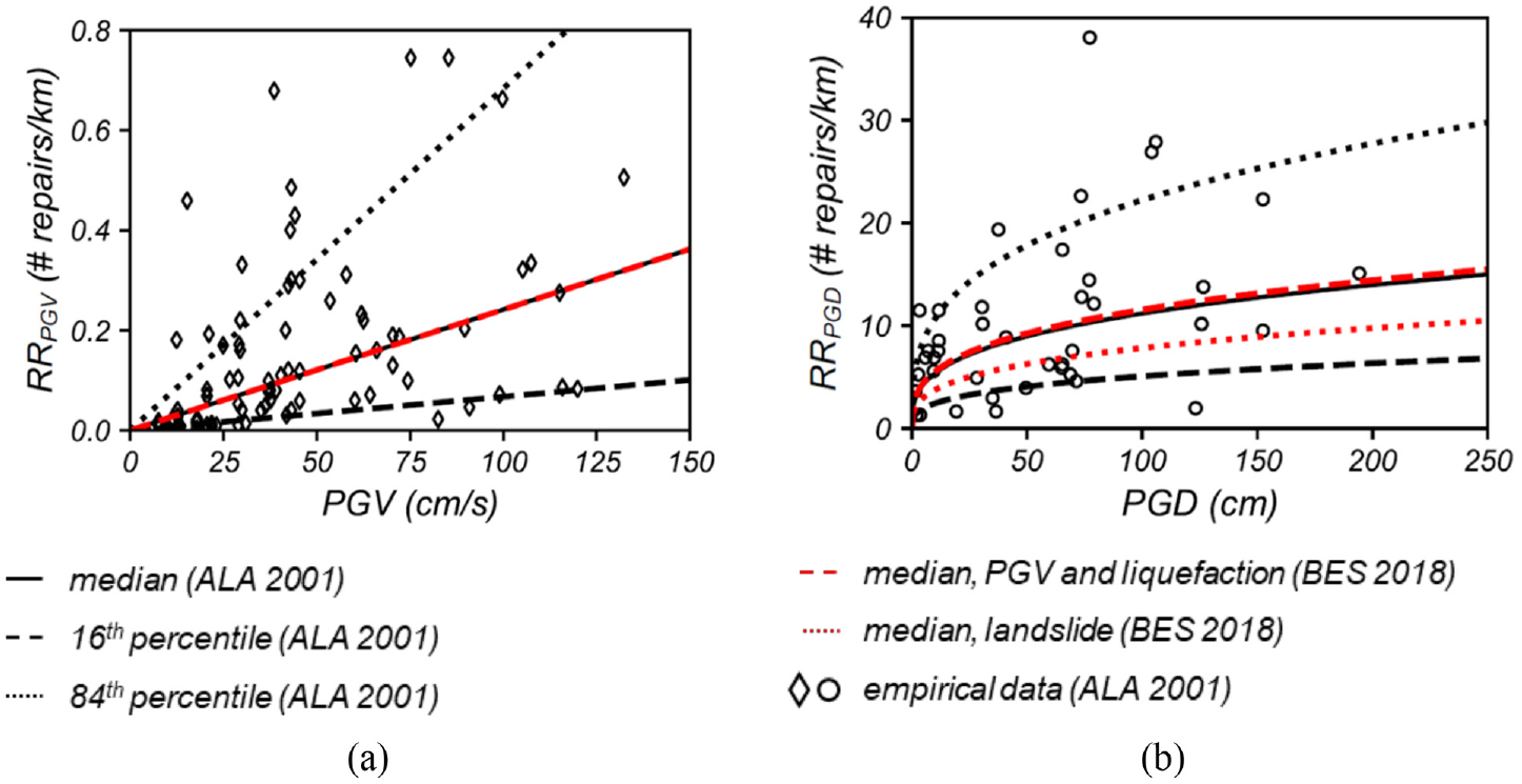
Repair rate relationships based on ALA (2001) and BES (2018a) fragility functions with respect to: (a) ground shaking, PGV, and (b) ground deformation, PGD. As an example, pipe diameters of 61 cm and depths of 2.1 m were used in the BES (2018a) liquefaction and landslide fragility functions, respectively.
The PGV-based fragility functions were developed based on a set of 81 data points in ALA (2001) from 12 historical earthquakes, with the majority of the data points gathered after the 1995 Kobe, 1994; Loma Prieta, and 1971; Northridge, 1989 San Fernando earthquakes. These data points correspond to pipe materials consisting of CI (47%), steel (16%), AC (13%), ductile iron (DI) (12%), concrete (CONC) (3%), or other (16%). Based on these data, the variability in PGV-based repair rates in Figure 1a was modeled using a lognormal fragility function with parameters
The PGD-based fragility functions were developed based on 42 data points in ALA (2001) gathered after four earthquakes, namely, the 1906 Nihonkai-Chubu, the 1989 San Fernando, the 1983 San Francisco, and 1971 Loma Prieta earthquakes. These data points correspond to pipe materials consisting of AC (48%), CI (40%), or mixed CI and steel (12%). To account for the variability in PGD-based repair rate, a lognormal fragility function was fit to the data of repair rate versus PGD in Figure 1b with parameters
Thus, the ALA (2001) fragility functions were modified to account for repair rate variability by:
where
Model class uncertainty
To account for the effects of model class uncertainty, recently developed pipe repair rate fragility functions by the City of Portland Bureau of Environmental Service (BES, 2018a) were compared to ALA (2001) in a sensitivity study. Ideally, model class uncertainty would incorporate multiple independently developed models; for example, using a weighted average or logic tree approach (Alam and Barbosa, 2018; Barbosa, 2011; Muto and Beck, 2008; Romano et al., 2021). However, due to the limited models available for wastewater networks, generic (i.e. ALA, 2001) and local, site-specific (i.e. BES, 2018a) models were used to characterize the sensitivity to model class uncertainty, herein.
In BES (2018a), formulations are developed for PGV- and PGD-related repair rates and divided into liquefaction-induced lateral spreading and ground settlement (LQ) and landslide-induced ground deformation (LS):
where D is the pipe diameter (cm) and h is the pipe depth (m). Although herein referred to as the BES (2018a) formulation, Equation 4 was only explored by BES for comparison purposes and final results and mapping in BES (2018a) were still based on ALA (2001).
Unlike the ALA (2001) formulations in Equation 2, the PGD-related repair rates in BES (2018a) explicitly account for pipe diameter and pipe depth, since larger-diameter pipes are typically located at greater depths in wastewater systems compared to potable water systems. From inspection of Equation 4c, the BES (2018a) function indicates that the probability of pipe repairs per unit length decreases with increasing pipe depth for landslide-based hazards. In Equation 4b, sensitivity to pipe diameter for liquefaction-based hazards is mainly associated with relatively small pipe diameters and the dependence of repair rate per unit length on pipe diameter plateaus for larger-diameter pipes. However, note that lower damage rates for large-diameter water pipes have been observed after past earthquakes (Eidinger, 1998; Giovinazzi et al., 2015; Nagata et al., 2011; O’Rourke and Jeon, 1999). To some extent, lower damage with increasing diameter can be attributed to the higher quality of construction, lower corrosion effect, fewer bends and tees, larger wall thickness, and so on commonly found for larger-diameter pipes compared to smaller diameter pipes. The flow conditions in water and wastewater system are fundamentally different, as there is pressurized flow for the former and more open channel flow for the latter; however, dependence on diameter could also be arguably based on the anecdotal evidence of the better performance of large-diameter water pipelines after past seismic events, and this effect is not considered in Equation 4b. The
Fragility modification factors k1 and k2 for different model classes

Source: BES (2018a) for wastewater pipelines.
Not originally suggested in ALA (2001). These values were assumed in the application of ALA (2001) for wastewater pipelines based on the values provided in BES (2018a).
BES (2018a) provides only median fragility functions for repair rate, without providing information on repair rate uncertainty. In the absence of such information, lognormal standard deviations of 1.15 and 0.74 were assumed for the
where
Correlation
In this study, model parameter uncertainty in each of the fragility model classes for pipe repair rate was accounted for by simulating the respective
To account for the spatial correlation of pipe damage in seismic events, spatial auto- and cross-correlations of pipe repairs were also considered when simulating the
Correlated RV generation
The eigenvalue analysis method for generating correlated RVs in Nowak and Collins (2012) was utilized to transform uncorrelated coefficients,
As this method is valid for normal distributions and approximate for other distributions, a new matrix of correlated RVs,
where
Spatial auto-correlation
At the time of this study, limited ground motion correlation models exist for PGV and are non-existent for PGD, which are the IMs used in the pipeline repair fragility models in Equations 3 and 5. Moreover, no spatial-correlation models for pipe damage currently exist in the literature.
In the absence of spatial-correlation models for ground motion IMs relevant to pipeline seismic response and for pipe repair, herein, the spatial-correlation model presented in DeBock et al. (2014) was adopted to model the spatial correlation of pipe repairs for a wastewater system. As DeBock et al. (2014) studied building story drift ratio response under seismic excitation, building response is being used in this study as a proxy for pipe repair rate. Future studies can better represent the spatial correlation of pipe repairs as additional damage information is collected and specific efforts are made to assess the spatial correlations of pipe repair rates (i.e. spatial similarity in pipe damage) in addition to the correlations associated with the IMs (e.g. from the wave propagation and uniformity of adjacent soil).
DeBock et al. (2014) studied the effects of spatial correlations in building response under ground shaking for four different earthquakes, including two historical events, 1994 Northridge (M6.7) and 1999 Chi-Chi (M7.6), and two simulated events, Puente Hills fault (M7.2) and ShakeOut (M7.8). The study used ground motion models (GMMs) and models of the spatial correlation of

Assumed bounds represented by gray block for the spatial auto-correlation of pipe repairs with increasing distance adapted from DeBock et al. (2014); i, ii, iii, and iv point to spatial cross-correlation bounds used in case study.
In this study, the lower and upper bounds of the correlation coefficients for story drifts presented in DeBock et al. (2014) were assumed to bound the potential spatial auto-correlation of a given wastewater pipeline system (see gray block in Figure 2); herein, linear regression was used to fit the building response correlation data from the ShakeOut and Puente Hills faults to determine lower- and upper-bound spatial auto-correlations,
To generate spatial auto-correlations, the intersite distance was computed based on the Euclidean distance between the geospatial midpoint locations of pipes
where
The spatial auto-correlation matrix,
where the diagonal block matrices,
Spatial cross-correlation
Compared to the spatial auto-correlations, which define correlations of pipe damage for similar pipe materials located at different distances, spatial cross-correlations define correlation of pipe damage for different pipe materials located at different distances. Naturally, the magnitude of cross-correlation is not as strong as that of auto-correlation for similar intersite distances. In DeBock et al. (2014), cross-correlations between story drifts for different buildings at the same site resulted in lower y-axis intercepts with similar diminishing trends with increasing distance compared to the spatial auto-correlations. Based on this observation, herein, the effects of spatial cross-correlation on the damage of pipes with different materials located at different sites assume that the spatial cross-correlation is the product of a material correlation,
In contrast to the spatial auto-correlation,
where the main diagonal block matrices,
Although not considered in this study, another form of correlation exists, that is, the correlation between
Component- and system-level pipe repairs
Two levels of pipe repairs were considered in this study: component- and system-level repairs. Component-level repairs represent the number of repairs over a pipe length. System-level repairs sum the fraction of repairs in each pipe for the entire pipeline network. In these calculations, the RVs,
At the component level, the number of repairs, or pipe repairs
where
To incorporate model class uncertainty, the pipe repairs can be weighted and summed for different model classes in Equation 10, where the subscripts
To compute the system-level repairs, or total number of system-level repairs (
where
To summarize, the total system-level repairs,
The repair data can be used to estimate the cost of repairing the damaged pipes in the wastewater network. The component-level loss
where
The component-level repair loss,
Note, Equation 12 assumes that pipe damage can be spot repaired by digging down and inserting a new pipe. Loss does not include costs associated with: (1) physical losses from emergency stabilization (e.g. traffic control and placing plate barricade over the sinkhole to ensure public safety and initiating bypass pumping to provide continuity of service), complicating factors of removing and replacing pipe in dense urban versus rural environments, grade correction and flowline restoration, changing the gravity system to a pressurized system (Liu et al., 2013), de-silting and inspection, relocating utilities, removal of liquefiable soils (Giovinazzi et al., 2015), interdependencies with critical assets of other utilities (e.g. utility crossing or parallel water line relocation), excess excavation and shoring required for pipe access, removal, and installation, or mitigation of failure due to buoyancy (BES, 2018b); (2) environmental losses from sewage spills from pipe leakage/breaks and over-dumping from non-functional sewer components into water sources, such as the waterway, ground surface, and fresh water (Liu, 2016); and (3) social losses that compromise general well-being due to the loss of sanitary services, households suffering from odorous issues, and flow blowbacks, which may force residents to temporarily move from their properties (Liu, 2016). In addition, some cost savings were neglected, such as those obtained by repairing pipes in close proximity to remediate multiple damage points.
Overview of methodology
Figure 3 shows the flowchart for computing component- and system-level repair and loss for a wastewater pipeline network based on the discussed sources of uncertainty and damage correlations. The following lists each step in the flowchart briefly, as detailed information for each step was described in the previous sections:

Flowchart for implementing the probabilistic methodology, including model parameter uncertainty, model class uncertainty, and pipe repair correlations.
Network information, such as pipe geospatial locations (e.g. start and finish nodes), average depth relative to the ground, and other attributes, including length, material, diameter, and connectivity, are collected for each pipe.
The hazard intensity maps geo-spatially define the IM, typically in terms of PGV or PGD maps and in the form of a GIS raster files. Through interpolation of the raster files,
Model parameter uncertainty is incorporated and propagated using MCS to account for uncertainty in the repair rates used in the fragility function models for the pipes. For each realization in the MCS, spatial auto- and cross-correlated sample variables for pipe repair rates are generated from uncorrelated sample variables based on intersite distances between pipe midpoints and differences in pipe materials:
For each pipe
For all pipes, the spatial auto- and cross-correlation
Correlated RVs
4. The number of repairs is calculated for each pipe using Equation 10 and summed to calculate the number of repairs for the pipeline system for each realization using Equation 11.
5. The loss is computed based on the estimated number of repairs for each pipe using Equation 12 and summed to estimate the loss of the pipeline system for each realization using Equation 13.
6. Statistical distributions are fitted to the pipe repair and loss realizations. These distributions can be used to compute the relevant statistics, including the mean, median, standard deviation, percentiles, or confidence interval (CI).
7. As needed, this process can be repeated for other models to incorporate model class uncertainty using Equation 10. Results of each MCS can then be combined using a weighted average or logic tree approach (Alam and Barbosa, 2018; Muto and Beck, 2008; Romano et al., 2021).
Other hazard intensity maps can also be included, repeating steps 1–7. The methodology can be further extended to obtain risk-based repair and loss estimates by weighing the results from various scenarios with mean annual rate of occurrence for each scenario.
Case study
To demonstrate the probabilistic methodology, the wastewater backbone system for the City of Portland, OR, USA was used as application case study. Wastewater networks are considered critical infrastructure per Presidential Policy Directive PPD-21 (American Water Works Association (AWWA), 2021; PPD-21, 2013); thus, network information and component-level repairs are presented in terms of four zones in the Portland area, as shown in Figure 4b, without explicitly showing the network. These zones were identified based on the expected IM maps of earthquake scenarios presented in section “Earthquake scenarios,” namely, (1) Zone-1: region near the Columbia River and other tributaries or creeks with extremely high liquefaction zones prone to PGD of 100 cm and higher; (2) Zone-2: region near the Willamette River with high-to-extremely high liquefaction zones prone to PGD of 50 cm and higher; (3) Zone-3: region near the Portland Hills with extremely high landslide zones prone to PGD of 100 cm and above; and (4) Zone-4: downtown flat topography zone with low-to-moderate PGD levels of 50 cm and lower.

Case study: (a) nearby faults to the wastewater network and (b) breakdown of wastewater network by different hazard exposure zones.
Wastewater backbone system
Although not shown herein, two major pipelines run parallel to the Columbia River along the NE Marine Drive and NE Lombard Street, and another two backbone tunnel lines run somewhat parallel to each side of the Willamette River. The backbone system was comprised of 440 km sewer pipes of different materials, sizes, and depth, with
Overall, 6.7%, 64.1%, 1.6%, and 27.6% of pipes fall into Zone-1, Zone-2, Zone-3, and Zone-4, respectively. Figure 5 shows network analytics of pipe materials, size, and depth in the different pipe Zones 1–4. Similar to the breakdown associated with the whole network, CSP is the major pipe material in all the zones (see Figure 5a). Notably, ductile iron pipes (DIPs) constitute 10% of Zone-1 materials, while VCP and HDPE pipes both constitute 6% of Zone-3 materials. Proportions of these pipe materials (i.e. VCP, HDPE) are considerably lower compared to the more prevalent concrete-based pipes in the network. As shown in Figure 5b, median pipe sizes for different zones are 0.76, 1.06, 1.06, and 0.92 m for Zones 1–4, respectively. Pipe sizes vary most in Zone-2 due to the existence of very large-diameter mains and tunnels. Median pipe depths (see Figure 5c) are similar across Zone-1 to -3 (of about 3.9 m), whereas median pipe depths are larger for Zone-2 and -4 (medians of 4.2 and 4.6 m, respectively). Like the pipe sizes, pipe depth varies most in Zone-2, between
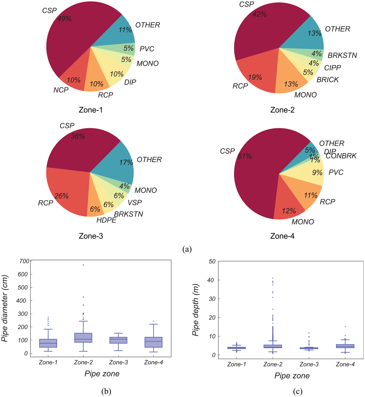
Wastewater network analytics by zone: (a) breakdown of major pipe materials, (b) distribution of pipe size,
Earthquake scenarios
The wastewater backbone system in the City of Portland is vulnerable to regional and local earthquakes (see Figure 4a). In this study, repairs for the wastewater network were assessed for deterministic earthquake scenarios originating at the CSZ, a 970-km (600-mile) long fault running in the Pacific coast from north of California, USA to British Columbia, Canada, and the Portland Hills fault, a local crustal fault located at the foot of the Tualatin mountains.
Four plausible CSZ expected IM maps were considered: M8.1, M8.4, M8.7, and M9.0. Of these, the M9.0 map was developed in Medina and Burns (2013) by the Oregon Department of Geology and Mineral Industries (DOGAMI). The other CSZ maps (for the M8.1, M8.4, and M8.7) were later developed by Sharifi Mood (2017) following the methods presented in Medina and Burns (2013). Past earthquakes along the CSZ fault have occurred at intervals varying from decades to centuries, ranging widely in magnitude and rupture location (Goldfinger et al., 2012; Oregon Seismic Safety Policy Advisory Commission (OSSPAC), 2013; Park et al., 2017). At least 40 large-magnitude earthquakes have occurred along the CSZ fault in the past 10,000 years, including (1) 19–20 full-margin or nearly full-margin ruptures, (2) 3–4 ruptures along 50%–70% of the southern Oregon margins, (3) 10–12 southern ruptures from central Oregon southward, and (4) 7–8 central Oregon/northern California ruptures (Goldfinger et al., 2012). The M8.1 map was based on simulating partial ruptures in southern Oregon and northern California, affecting the southern Oregon coast with shaking intensities of PGA = 0.5–0.55 g, resulting in little effect in the Portland region (shaking intensities with PGA < 0.05 g). In contrast, the M8.7 and M9.0 maps were estimated based on the CSZ full rupture, with the M8.7 producing higher shaking intensities near Coos Bay along the southern Oregon coast and the M9.0 producing shaking over a larger geographical area from the coast to the Cascade Range (Madin and Burns, 2013).
An expected IM map for the M6.8 Portland Hills fault was determined in Bauer et al. (2018). Although the CSZ maps affect larger geographical regions, the Portland Hills fault map is more impactful to the case study network given the proximity of the fault relative to the site. Note, the likelihood of a Portland Hills fault earthquake is considerably lower than a CSZ earthquakes (Bauer et al. 2018), with evidence suggesting two ruptures in the past 15,000 years (Liberty et al., 2003).
In the development of expected IM maps, Sharifi Mood (2017) and Bauer et al. (2018) utilized the Boore and Atkinson (2008) GMM to estimate PGV and the HAZUS-MH (FEMA, 2010) ground deformation models to estimate PGD. For the PGD hazard maps, Bauer et al. (2018) considered “dry” and “wet” conditions to reflect soil moisture content due to landslide and liquefaction. As the more severe scenario, the “wet” condition PGD hazard maps for the Portland Hills fault event were considered in this study. Note, the Boore and Atkinson (2008) GMM model accounts for relevant sources of uncertainty in the IM arising from source, propagation, and site effects, using earthquake-to-earthquake (inter-event) and site-to-site (intra-event) variability components in the model. However, spatial correlation of IMs was not considered in determining the site-to-site IM variability. However, the HAZUS-MH ground deformation models estimate PGD values accounting for liquefaction-induced lateral spreading and landslide-induced ground failure, along with a probability of their occurrence. The CSZ scenario maps, which were intended for state-wide seismic risk applications, such as the ones developed in Burns et al. (2021), were developed at 30 m resolutions, whereas much finer resolutions were used for Portland Hills fault scenario for its potential application in the three counties surrounding Portland, OR (9 m for PGV and 3 m for PGD).
Figure 6 shows the expected PGV and PGD values for the M6.8 Portland Hills fault and CSZ M9.0 scenarios. As evident in these figures, the local crustal event (M6.8 Portland Hills) results in more severe and varied IMs compared to distant subduction zone events (CSZ M9.0). Using these hazard maps, PGV and PGD at the pipe midpoint locations were extracted from the respective scenario raster files using a Python script developed with the Rasterio (2022) library. Note, as wastewater pipelines are mainly gravity systems, the pipe depth likely varies with length and may not be well represented by the pipe midpoint. Multiple points along the pipe length could alternatively be utilized. Approximately 72.6% of the backbone system (6.7% in Zone-1, 64.1% in Zone-2, and 1.6% in Zone-3) lies in high-to-extremely high PGD hazard zones exceeding PGD of 50 cm, either due to liquefaction or landslide-induced ground deformation for the CSZ M9.0 event (Figure 6e and f). Concentrations of service laterals may also be higher in downtown flat topography, even though this study focuses on service mains.
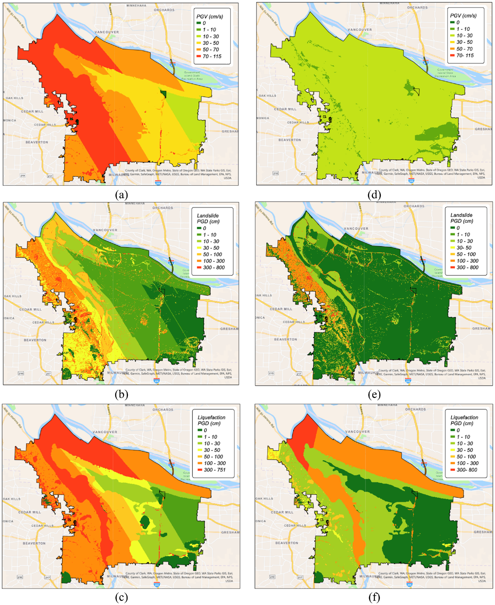
Considered expected IM maps: (a) PGV, (b) landslide-induced PGD, and (c) liquefaction-induced PGD maps for Portland hills fault M6.8 scenario; (d) PGV, (e) landslide-induced PGD, and (f) liquefaction-induced PGD for CSZ M9.0 scenario.
Repair and loss calculations
In a scenario-based assessment, the probabilistic methodology was used to study component- and system-level repairs and loss of the case study wastewater pipeline network. Uncorrelated variables were generated for each pipe using the lognormal distributions for
After a seismic event, loss would likely be associated with: (1) physical loss, (2) environmental loss, and (3) social loss (Liu, 2016). Limited cost data were available for the case study wastewater network. Thus, loss was characterized only by the physical loss due to damaged pipes, with the component- and system-level losses estimated using Equations 12 and 13, respectively.
Since it was expected that damaged pipes could eventually be replaced with more modern pipe designs and materials, estimates of loss were based on hypothetical approaches explored by wastewater professionals at the Bureau of Environmental Science (BES), City of Portland, OR, USA. Based on their guidance, pipe repairs/replacements were categorized as: (1) replacement of damaged pipes of diameter
Per unit costs from this memorandum included cost estimates associated with pipe materials, installation, and surface restoration for pipes of different materials and installation depths. To account for the additional excavation needed for adequate access to the damaged pipes, per unit length repair costs were adjusted with a pipe access length factor,
Results and discussion
Results are presented and discussed in terms of: (1) model parameter uncertainty, (2) sensitivity to model class, (3) correlation (spatial auto- and cross-correlation), (4) deterministic earthquake scenarios, and (5) loss. For brevity, most results are presented in terms of the total system-level pipe repairs (TSR) using the ALA (2001) fragility functions for the M9.0 CSZ scenario. Results from the BES (2018a) model class and the other scenarios (M6.8 Portland Hills Fault, M8.1, M8.4, and M8.7 CSZ events) are shown where comparisons are needed. In particular, results are presented in terms of their relevant statistics, such as the mean, median, standard deviation, CI of the mean, and most likely spread, measured in terms of 16th and 84th percentile bounds of the TSR. The CIs of the mean of the lognormally fitted TSR values were computed using the Cox method (Olsson, 2005).
Effects of model parameter uncertainty
Figures 7 and 8 show the effects of including model parameter uncertainty on the system- and component-level pipe repairs, respectively, for the CSZ M9.0 scenario using the ALA (2001) fragility functions. In these figures, uncorrelated
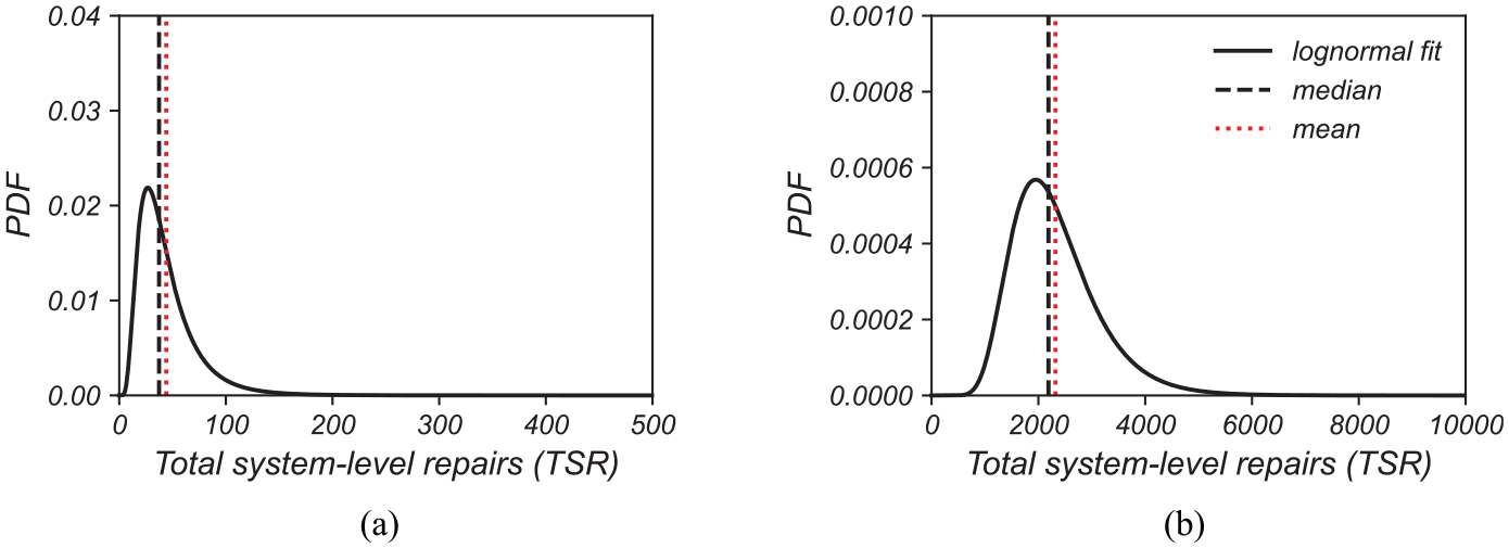
Effects of model parameter uncertainty on the total system-level repairs (
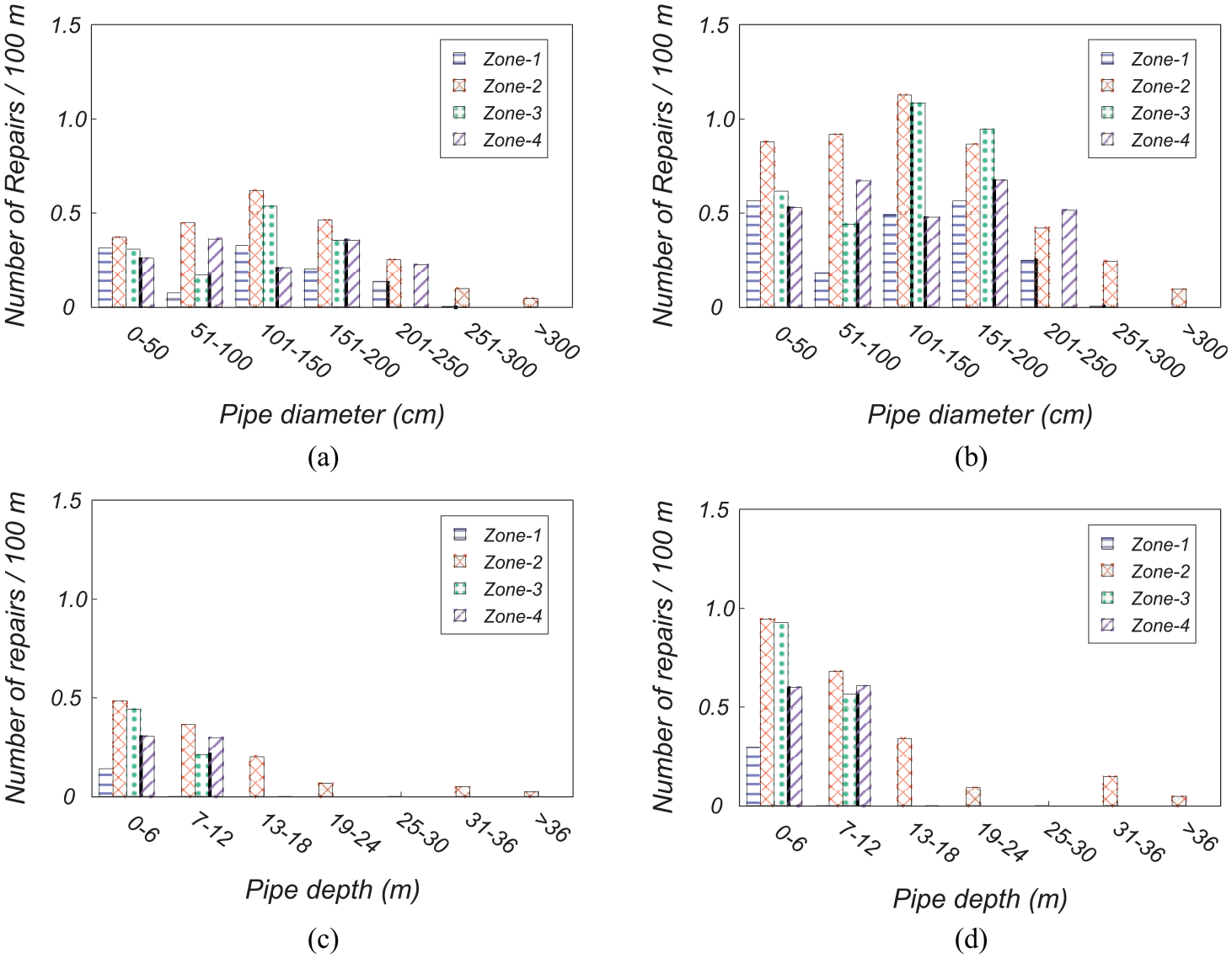
Component-level repairs by pipe zone for the M9.0 CSZ scenario using the ALA (2001) PGD-based model: (a) and (c) 16th percentile and (b) and (d) 84th percentile realizations of the total system-level repairs (
System-level pipe repairs (
)
Figure 7a and b shows the probability density functions (PDFs) for the total system-level repairs (
Median and mean estimates are shown by vertical dashed and dotted lines, respectively. For PGV-related repairs, the median TSR and log standard deviation were 37.5 and 0.58, respectively. In contrast, for PGD-related repairs, median TSR and log standard deviation were 2190 and 0.34, respectively. The most likely spread of repairs using the 16th and 84th percentile values of TSR were (21.5, 65) and (1560, 3060) for PGV- and PGD-based hazards, respectively.
To gain insight, PGV was relatively small for the case study network (about 10–30 cm in Figure 6d), since the M9.0 is relatively far from Portland. Thus, PGV resulted in smaller estimated damage (mean of 44 TSR, 95% CI of the mean of (43.5, 45.7)). In contrast, damage estimates were larger and more varied for the PGD hazard (mean of 2320 TSR, 95% CI of the mean of (2303, 2336)) due to a combination of: (1) high PGD levels due to large magnitude and significant duration effects and (2) higher exposure of pipes, since about 72.6% of the backbone system is located in high-to-extremely high liquefaction and landslide prone areas with PGD > 50 cm (6.7% in Zone-1, 64.1% in Zone-2, and 1.6% in Zone-3 in Figure 6e and f). Note, however, the probability of observing large values of TSR at the tail end of the distribution is extremely low for both ground shaking and ground deformation hazards.
Component-level pipe repairs (
)
Figure 8 shows snapshots of the component-level repairs (
In general, component-level repairs increase with the increasing TSR percentile levels, irrespective of pipe size and depth. With respect to pipe size (see Figure 8a and b), the following can be observed: (1) number of repairs/100 m is the highest for Zone-2 compared to the other zones, irrespective of pipe size and system-level TSR percentile levels and (2) number of repairs/100 m decreases with pipe size for pipes greater than 100 cm in diameter for pipes in Zone-2, although a general trend cannot be established for the other zones for similar pipe sizes. Further investigation and data collection are needed after future events to validate whether a correlation exists between pipe size and their vulnerability, especially since very large-diameter pipes (greater than 250 cm diameter) are only located in Zone-2 and other factors (e.g. IM) may also play an important role.
With respect to pipe depth (see Figure 8c and d), the following can be observed: (1) pipe vulnerability is the highest for pipes located in Zone-2 compared to other zones due to higher levels of liquefaction-induced lateral spreading and (2) pipe vulnerability decreases with increasing pipe depth for all pipe zones. Specifically, pipe vulnerability decreases significantly for pipes located in soil deeper than 10 m, as those pipes are likely to have significant overburden pressure and less likely to sustain lateral deformations even if located near liquefaction zones, such as Zone-2, which is close to the Willamette River (see Figure 6f).
Sensitivity to model class
Figure 9 shows the sensitivity of the
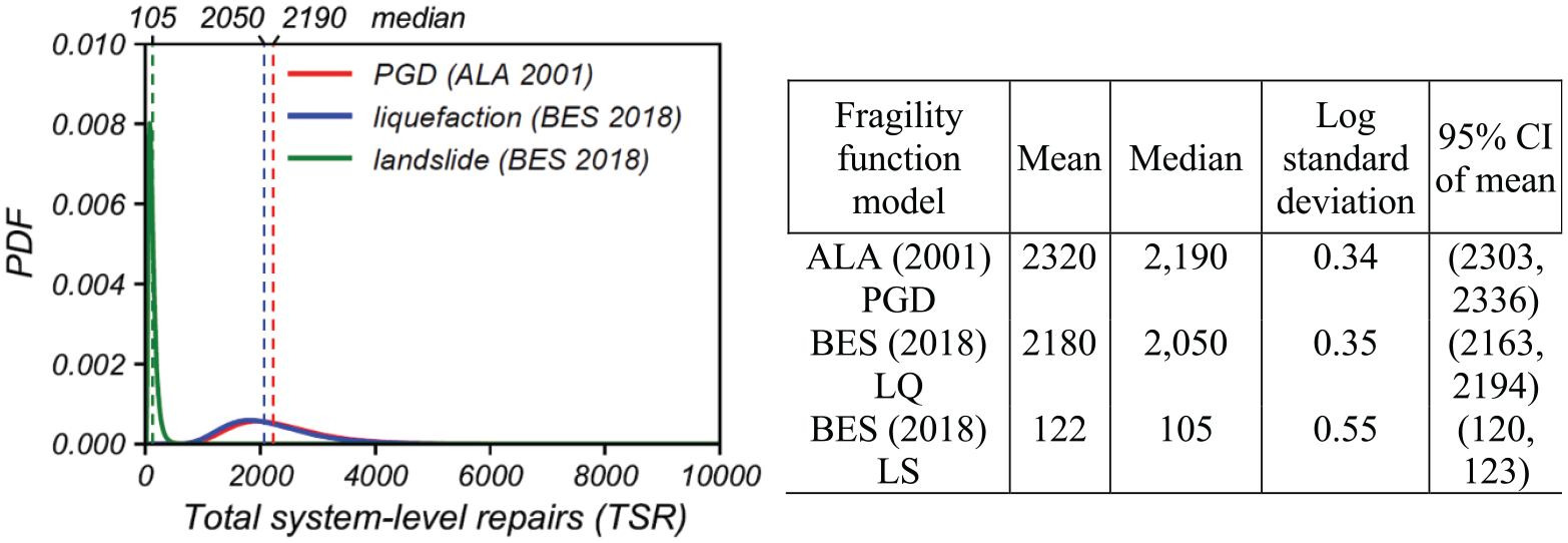
Effects of model class uncertainty on the total system-level repairs (
The PDFs of the TSR for the ALA (2001)-PGD and BES (2018a)-liquefaction (LQ) models are quite similar, as shown in Figure 9. The ALA (2001) mean and median estimates of TSR were slightly larger with respect to the corresponding BES (2018a)-LQ mean and median estimates of TSR. There is convincing evidence that the mean difference between the TSR computed using ALA (2001) and the BES (2018a)-LQ is non-zero (two-sided p-value < 0.01 from a paired t-test). Larger mean and median TSR for the ALA (2001) model are expected compared to the BES (2018a)-LQ model, as ALA (2001) lumps liquefaction and landslide-induced repairs together. The BES (2018a) formulations reveal that PGD-induced repairs are governed by liquefaction compared to landslides for the case study, which is consistent with the comparatively larger and more widely spread liquefaction hazard in Zone-1 and Zone-2 of the case study area in Figure 6 for the CSZ M9.0 event.
Effects of correlation
Figure 10 shows the effects of considering spatial auto- and cross-correlation of pipe repair rates on the TSR for the CSZ M9.0 event using ALA (2001).
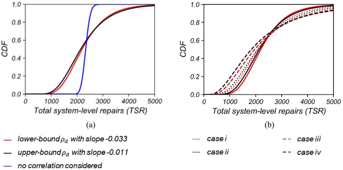
Effect of spatial correlation
Effects of spatial auto-correlation
Figure 10a shows the effects of considering spatial auto-correlations,
Effects of cross-correlation
Figure 10b shows the effects of considering cross-correlations on the CDF of the
The different spatial cross-correlation cases (cases i–iv) resulted in observations similar to those of the spatial auto-correlations, but with greater effect on the CDF of the TSR; that is, observations (i), (ii), and (iii) from section “Effects of spatial auto-correlation” still hold but become more apparent. The following statistics were obtained for the four levels of cross-correlation considered: (1) mean TSR of 2362, 2351, 2342, and 2296; (2) log standard deviation of the
Effects of earthquake scenarios
Calculations for the
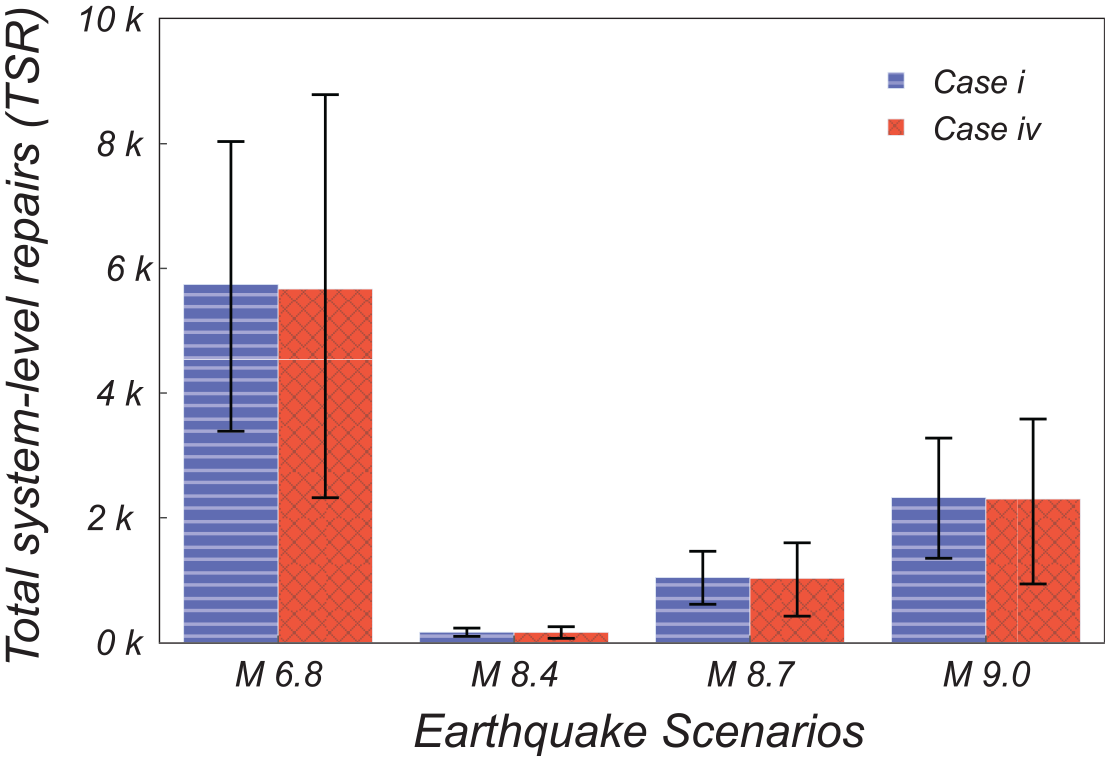
Effects of earthquake scenario on the total system-level repairs (
Figure 11 shows the effects of varying earthquake scenarios on the system-level repairs (
Loss estimation
Figure 12 shows mean estimates of the system-level loss
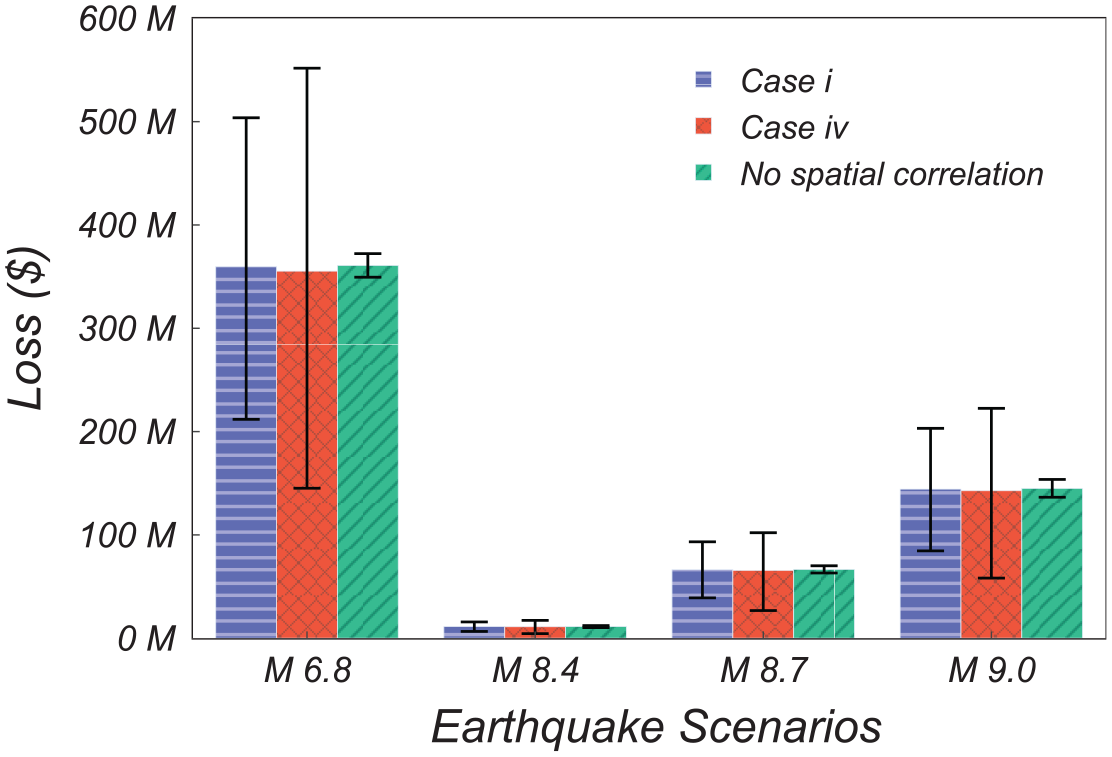
Estimates of seismic loss for different earthquake scenarios for PGD-induced damage using ALA (2001) for different pipe repair rate correlation levels. Colored bars represent the mean loss estimates, and black line bounds represent the spread of the estimated loss (defined by the 16th and 84th percentile loss bounds). Cross-correlation cases “i” and “iv” of
For the CSZ M9.0 event, the 95% CI of the mean system-level loss was ($142.8, $145.5) and ($140.4 M, $144.7M) for the low- and high-levels of cross-correlation, respectively. The corresponding estimates of spread for the TSR were ($84.5M, $203.1M) and ($58.2M, $222.5) for the low- and high-levels of cross-correlation, respectively. Note, the system-level loss was computed using Equation 13, which incorporates adjustments for additional excavation beyond the pipe repair length to access the damaged pipes, repair cost inflation, emergency contingencies during post-disaster response, and design and administrative fees. For low-levels of cross-correlation, a 95% CI of the mean TSR of (2337, 2373) translates to mean repair costs of about $62K for each instance of repair in the network. For high-levels of correlation, a 95% CI of the mean TSR of (2262, 2331) also translates to about $62K for each instance of repair, similar to the low-levels of spatial cross-correlation.
In contrast, for the local M6.8 Portland Hills scenario, the 95% CI of the mean system-level loss was ($356.2M, $362.9M) and ($349.5M, $360.3M) for low- and high-levels of cross-correlation, respectively. The corresponding estimates of spread for the TSR were ($211.8M, $503.7M) and ($145.1M, $551.7M) for low- and high-levels of cross-correlation, respectively. The cost of each repair for the M6.8 Portland Hills shaking was similar to that of CSZ M9.0 shaking, irrespective of spatial-correlation levels.
It is evident in Figure 12 that, for a given earthquake expected shaking map, system-level loss varies considerably depending on the level of spatial cross-correlation, but the mean loss remains essentially unaltered. These observations are consistent with the properties of the lognormal RVs discussed in section “Component- and system-level pipe repairs,” where the mean of the sum of lognormal RVs decreases and variance increases with higher correlation levels, respectively. While the mean loss remains essentially unchanged for this case study network, the effects of including correlations may be larger or smaller in future studies depending on the considered damage correlation model and other sources of uncertainty, which could overshadow the effects of the correlations.
Note, pipe replacement over a few blocks can cost millions of dollars, and pipe replacements downtown can cost multiples of millions of dollars under ideal conditions. As described in section “Component- and system-level pipe repairs,” the projected loss calculated per Equation 13 provides only order-of-magnitude estimates. Estimates of system-level loss would improve with more detailed cost data, refined repair definitions for the fragility functions, and, ideally, the development of data-driven spatial-correlation models of pipe network damage based on future seismic events.
Summary and conclusions
A probabilistic methodology for damage (defined by the number of pipe repairs) and loss assessment of a wastewater pipeline network subjected to multiple deterministic earthquake scenarios was presented. The methodology incorporates multiple sources of uncertainty (e.g. model parameter uncertainty and model class uncertainty) and pipe repair rate correlations (e.g. spatial auto- and cross-correlation) to estimate the number of repairs of a wastewater pipeline network and to characterize the loss associated with pipe replacement costs, which traditionally have not been considered. The methodology was applied to a case study wastewater network in Portland, OR, using expected hazard intensity maps of multiple deterministic earthquake scenarios, including CSZ M8.1, M8.4, M8.7, and M9.0 and local crustal Portland Hills M6.8 events. The number of repairs and loss was evaluated using model parameter uncertainty, and their sensitivity to model class uncertainty was assessed using two fragility function model classes ( ALA 2001; BES, 2018a) and multiple levels of spatial and cross-correlations of pipe repair rates, representing assumed lower and upper bounds of repair estimates. Summaries and key findings include the following:
Incorporating modeling uncertainty in pipe fragility functions, which is typically neglected, enables estimates of the dispersion of pipe repairs in addition to a single mean and median estimate. For example, for the case study wastewater network, using uncorrelated variables and ALA (2001) fragility functions, the most likely spread (defined by the 16th and 84th percentile TSR bounds) of the total number of repairs could vary between 21.5 and 65.0 TSR and 1564–3060 TSR for the CSZ M9.0 event and PGV and PGD hazards, respectively.
Sensitivity to model class uncertainty, which arises from the use of different fragility models, contributed to uncertainties in the component- and system-level repairs. The PDF of the system-level repairs estimated using the BES (2018a) fragility model, including liquefaction, was comparable to the ALA (2001) PGD-based model, with the slightly larger ALA (2001) estimates, because the ALA PGD-based model combines liquefaction- and landslide-induced repairs. Use of BES (2018a) revealed that liquefaction-induced repairs contributed more than landslide-induced repairs for the case study. Although the two models are similarly formulated, there was evidence that the mean difference between the two models is non-zero (p-value < 0.01 from a paired t-test). Larger variations could occur for other site locations or hazards. Extensions to incorporate model class uncertainty could combine the results of multiple models using a weighted average or logic tree approach (Alam and Barbosa, 2018; Muto and Beck, 2008; Romano et al., 2021), as shown in Equation 10.
Component-level repairs, which were presented in terms of repairs/100 m deaggregated by pipe size and pipe depth for several hazard zones, revealed that (1) the number of repairs/100 m was estimated to be largest in Zone-2 compared to the other zones, irrespective of pipe size and depth, due to liquefaction-induced lateral spreading along the Willamette River, (2) pipe vulnerability decreases with increasing pipe depth for all hazard zones, with lower vulnerability for pipes located at 10 m or deeper depths, and (3) pipe vulnerability decreases with pips size for pipe diameters greater than 100 cm for pipes in Zone-2, although a general trend cannot be established for the other zones for similar pipe sizes.
Multiple sources of correlation in pipe repair rates, including spatial auto- and cross-correlations, were considered to illustrate their effects on estimates of system-level pipe repairs and loss. As a spatial-correlation model for pipe network damage did not exist in the literature at the time of this study, a lower- and upper-bound correlation structure of pipe repair rates was inspired by the spatial-correlation results presented in DeBock et al. (2014) for spatially distributed building response. Irrespective of the correlation source, observations included: (i) the mean and median TSR decreases with increasing correlation, (ii) the log standard deviation and spread of the TSR increases with increasing correlation, (iii) TSR is smaller for lower percentiles of repairs (e.g. for the 16th percentile) and larger for higher percentiles of repairs (e.g. for the 84th percentile) with decreasing correlation, and (iv) irrespective of correlation type, the effect of changing the correlation on the TSR statistics is the largest for the log standard deviation, followed by the spread and mean of the TSR. In addition, spatial cross-correlations of pipe repair rates had a more pronounced effect on the estimates of pipe repairs compared to the spatial auto-correlations. Note, observations (i)–(ii) may be artifacts of the statistical properties of the parameters used for the system-level pipe repair, which were modeled as the linear function of lognormally distributed component-level pipe repairs presented in section “Component- and system-level pipe repairs.”
System-level loss varied considerably depending on the earthquake magnitude, assumed level of correlation, and level of detail in the repair cost data. Estimates of the system-level loss would improve with more detailed cost information data, refined repair and stabilization definitions for the fragility functions, and future development of spatial-correlation models of pipe network damage. In addition, a more refined assessment of the wastewater system, including modeling assets such as inceptors, tunnels, service laterals, manholes, for example, as well as damage due to uplift and floatation, would affect the loss values presented herein.
The local crustal M6.8 Portland Hills fault scenario indicates comparably worse consequences compared to the CSZ M9.0 scenario, as shown by the system-level damage and loss results. However, the likelihood of occurrence for an M6.8 event is considerably lower compared to the CSZ cases. Future studies should incorporate PSHA instead of the scenario-based assessment performed herein to deaggregate risk by scenario to aid utilities in developing appropriate risk-consistent mitigation strategies.
Importantly, results of the case study revealed that different levels of spatial correlation of pipe repair rates could lead to different probabilistic estimates of damage and loss at the system level, although point estimates, such as the mean and median, remain essentially unaltered. Including modeling uncertainty can then aid decision-makers in making more informed decisions about possible lower and upper bounds of damage and loss for wastewater networks.
The presented probabilistic methodology is the first step toward the performance-based assessment of wastewater systems, where all relevant sources of uncertainty and correlation in pipe repairs are explicitly considered. Component- and system-level repair and loss assessments incorporating relevant sources of uncertainty, repair rate correlation, and deaggregation of damage, in terms of pipe size and depth for different pipe zones and several scenarios, would inform decision-making for: (1) developing zone-specific and phased capital investment and mitigation plans and (2) long-term worst case scenario planning. To develop system risk curves, the probabilistic methodology can be extended by incorporating additional probabilistic hazard definitions and sources of IM spatial correlations due to certain features of the earthquake (e.g. spatial correlations caused by high stress drop earthquakes) as an alternative to the expected IM maps used in this study. With a more recent paradigm shift toward hazard-resistant intelligent piping technology (Pacific Earthquake Engineering Research Center (PEER), 2019; Simpson et al., 2015; Steinbauer, 2021; Zhang et al., 2019), using advanced sensing technologies instrumented to collect spatially correlated data will also eventually lead to improved probabilistic assessments of seismic damage and loss and better risk-informed decision-making.
Footnotes
Appendix 1
Declaration of conflicting interests
The author(s) declared no potential conflicts of interest with respect to the research, authorship, and/or publication of this article.
Funding
The author(s) disclosed receipt of the following financial support for the research, authorship, and/or publication of this article: This study was funded by the Cascadia Lifelines Program ( ). The authors also express their sincere gratitude to Bureau of Environmental Science (BES), City of Portland for providing the wastewater backbone network and technical support regarding the system’s seismic vulnerability and wastewater pipeline repair process. Support for the third author was partially provided as part of the cooperative agreement 70NANB15H044 between the US National Institute of Standards and Technology (NIST) and Colorado State University through a subaward to Oregon State University. The content in this paper includes the views of the authors and does not necessarily represent the opinions or views of BES, City of Portland, NIST, or the US Department of Commerce.