Machine learning–based ground motion models for shallow crustal earthquakes in active tectonic regions

Abstract

Data-driven ground motion models (GMMs) for the average horizontal component from shallow crustal continental earthquakes in active tectonic regions are derived using a subset of the Next Generation Attenuation (NGA)-West2 data set, including 14,518 recordings out of 285 earthquakes recorded at 2347 different stations. We use four different nonparametric supervised machine learning (ML) algorithms including Artificial Neural Network (ANN), Kernel-Ridge Regressor (KRR), Random Forest Regressor (RFR), and Support Vector Regressor (SVR) to construct four individual models. Then, we use a weighted average ensemble approach to combine these four models into a robust model to predict various ground motion intensity measures such as peak ground displacement (PGD), peak ground velocity (PGV), peak ground acceleration (PGA), and 5%-damped pseudo-spectral acceleration (PSA). The model input parameters are moment magnitude, rupture distance, V_S₃₀, and Z_TOR. The ensemble modeling attempts to remove the drawbacks or deficiencies of different ML algorithms while capturing their advantages and accounts for epistemic uncertainty. Although no functional form is provided, the model can capture salient features observed in ground motions such as saturation as well as geometrical spreading, anelastic attenuation, and nonlinear site amplification. The response spectra and the magnitude, distance, V_S₃₀, and Z_TOR scaling trends are consistent and comparable with the NGA-West2 GMMs including several additional input parameters. We used a mixed-effects regression analysis to split the total aleatory uncertainty into between-event, within-station, and event-site–corrected components. The model is applicable to magnitudes from 3.0 to 8.0, rupture distances up to 300 km, and spectral periods of 0 to 10 s.

Keywords

Ground motion model seismic hazard analysis machine learning ensemble model mixed-effect regression

Introduction

Within active tectonic regions, there is ongoing deformation and movement of the Earth’s crust because of tectonic activities that can result in earthquakes or volcanic eruptions. The movement of tectonic plates leads to the accumulation of stress along fault lines that can produce shallow crustal earthquakes, generally with hypocentral depths of less than 25 km. Because these areas are prone to suffer from large devastating earthquakes, understanding the pattern and characteristics of earthquakes and predicting the expected level of shaking for a future event can significantly mitigate earthquake-related risks.

Ground motion models (GMMs) predict the expected level of ground motion shaking as a function of predictor variables such as earthquake magnitude, site-to-source distance, and site parameters. Thus, GMMs are widely used for seismic hazard analysis and risk assessment. Hundreds of GMMs have been developed for different regions and based on various data sets (Douglas, 2003, 2011). Conventional empirical GMMs are derived from observed ground motion recordings and have a closed-form functional form that estimates various ground motion intensity measures (GMIMs) such as peak ground acceleration (PGA) and 5%-damped elastic pseudo-spectral acceleration (PSA) at different periods as well as peak ground velocity and displacement (PGV and PGD). The development of traditional empirical GMMs is not a simple curve fitting, but it is a model building that uses recorded ground motions as well as results from seismological and geotechnical numerical simulations such as the hanging wall scaling, large magnitude scaling, and nonlinear site response scaling (Collins et al., 2006; Donahue and Abrahamson, 2014; Kamai et al., 2014). Developed GMMs such as the Next Generation Attenuation (NGA)-West2 GMMs (Abrahamson et al., 2014; Boore et al., 2014; Campbell and Bozorgnia, 2014; Chiou and Youngs, 2014; Idriss, 2014) are complex compared to other developed GMMs including complicated combinations of explanatory variables. These complicated combinations of explanatory variables, in addition to several constraints corresponding to numerical simulations, such as nonlinear site effects, hanging wall–footwall source effects, and basin-related site amplifications, may result in overfitting, limiting the predictive power of GMMs for future events (Bindi, 2017). Thus, the development process occurs in a series of steps within which model components are progressively constrained and/or smoothed to account for meaningful trends in the data as well as to avoid trade-offs in model coefficients (Parker et al., 2022).

Recently, machine learning (ML) approaches have been getting much attention as the size of databases for developing GMMs is increasing, particularly for tectonically active areas such as California, where plenty of strong ground motion data is available. These fully data-driven ML techniques can learn complex linear and/or nonlinear trends in high-dimensional data. ML is a part of artificial intelligence that enables computers to learn relationships and patterns in data without requiring any predefined functional form. Generally, ML algorithms are classified as supervised learning and unsupervised learning in which the outputs are labeled/known and unlabeled/unknown, respectively. Regression is considered a supervised ML class where the output is known as continuous numerical values. In this study, we use four well-known supervised nonparametric ML algorithms, including Artificial Neural Network (ANN), Kernel-Ridge Regressor (KRR), Random Forest Regressor (RFR), and Support Vector Regressor (SVR) as an alternative to classical regression techniques. In the following sections, we describe the data set selected for the analysis and provide some background about individual models. A grid search is performed to determine the best set of each model’s hyperparameters. Then, we use ensemble modeling to combine individual models into a final model to improve the accuracy and robustness of estimations for future events. The model is trained using a subset of the NGA-West2 data set to estimate PGD, PGV, PGA, and 5%-damped PSA values at 21 spectral periods from 0.01 to 10 s. The global GMMs developed in this study can capture significant features of earthquake phenomena such as magnitude and distance scaling, saturation effects, geometrical spreading, anelastic attenuation, and nonlinear site effects without defining any functional form. We compare our models with the NGA-West2 GMMs and show consistent magnitude, distance, V_S₃₀, and Z_TOR-dependence relations. We then use a mixed-effects regression analysis to determine the between-event, site-to-site, and event-site–corrected components that are required for performing site-specific probabilistic seismic hazard assessment (PSHA).

It should be noted that the goal of developing a new set of GMMs for a given region or a given data set is not to develop the best model to reject or supersede the other models but to propose another correct view and at the same time, different than the other GMMs developed for that data set. In this way, we can account for uncertainty in the model development process because of limited knowledge and the randomness of earthquake phenomena. For instance, the United States Geological Survey (USGS) uses a logic tree considering all five NGA-West2 GMMs with an assigned weight for each branch to capture the uncertainty in ground motion estimation. Different GMM ranking schemes (e.g. Kale and Akkar, 2013; Mak et al., 2017; Scherbaum et al., 2009) indicate that none of the developed GMMs is perfect in the entire range of magnitude, distance, and period for future earthquakes. In other words, some GMMs perform better in some periods, whereas others may perform better in other periods. Even sometimes, some GMMs perform better for a range of M-R; while for another M-R range, they may not provide the best estimation. Comparing the distance scaling curves with the observed ground motions from the 2019 M7.1 Ridgecrest and the 2023 M7.8 Turkey earthquakes, we show that our GMMs outperform for the mid-range period (∼1 s) for active shallow earthquakes. In addition, although our proposed GMMs have fewer explanatory variables included compared to NGA-West2 GMMs, the results are comparable and, in some periods, better match with the observed data compared to the NGA-West2 GMMs. This is useful for quick estimation of GMIMs (e.g. ShakeMap) after an earthquake where obtaining Z_1.0 (or Z_2.5 for basin depth), dip angle, the width of the fault, being a hanging wall site or not, and rake angle (for R_x and R_y₀ estimation) are more challenging than obtaining M, Z_TOR, V_S₃₀, and distance.

Ground motion database

The NGA-West2 database is an extension of the NGA-West1 database that includes a set of small-to-moderate magnitude earthquakes in California between 1998 and 2011 and worldwide strong ground motion data in active tectonic regimes post-2000 recorded from shallow crustal earthquakes (Ancheta et al., 2014). This database has been compiled by Pacific Earthquake Engineering Research Center (PEER) NGA to collect uniformly processed time series and response spectral ordinates for developing GMMs for shallow crustal earthquakes in active regions (Bozorgnia et al., 2014). This database collects instrument-corrected median orientation-independent horizontal component (RotD50, the 50th percentile of the response spectra over all nonredundant rotation angles; Boore, 2010) GMIMs with the corresponding earthquake and site condition characteristics within several active regions such as California, China, Greece, Iran, Italy, Japan, New Zealand, Taiwan, and Turkey. The updated flatfile released in 2015 (see section “Data and resources”) includes 21,540 recordings from 607 earthquakes. The following criteria are applied to the full data set to select a subset for use in the development of GMMs in this study:

Remove recordings with unknown/missing key metadata (magnitude, distance, Z_TOR, V_S₃₀, and PGA/PSA);

Remove ground motions with magnitudes less than 3.0 and rupture distances more than 300 km;

Remove ground motions with the multiple-event flag equal to 1;

Remove recordings with late P-trigger;

Remove aftershocks within a cut-off distance of 5 km from the main shock due to having below-average short-period amplitudes (Wooddell and Abrahamson, 2014);

Remove a few records that in the initial analysis are recognized as clear outliers (residuals in log scale larger than 4);

Finally, events with at least five recordings per event are kept in the final data set.

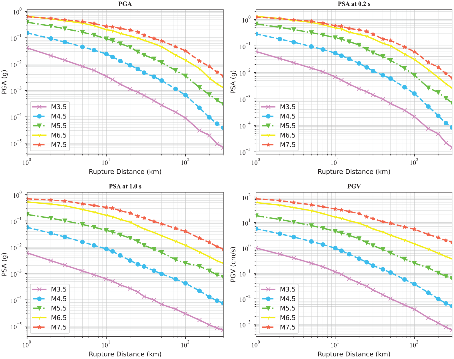
The final selected subset consists of 14,518 recordings from 285 events recorded at 2347 stations. Figure 1 shows the histogram distributions of magnitude, rupture distance, V_S₃₀, and Z_TOR, as well as the magnitude–distance distribution. There is good coverage for magnitude and distance; however, the majority of the data have magnitudes less than 5 and distances less than 100 km. Also, although V_S₃₀ values vary from 106 to 2016 m/s, the number of stations with V_S₃₀ less than 150 m/s or more than 1500 is very small. Figure 2 illustrates the distance scaling of the recorded ground motions for PGA, PSA at 0.2 and 1.0 s, and PGV. It is clear that PGA, PSA, and PGV strongly correlate with magnitude and distance.

Figure 1.

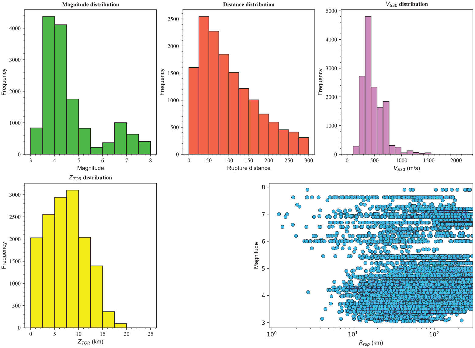
Distribution of the data used in terms of M, R_rup, V_S₃₀, and Z_TOR.

Figure 2.

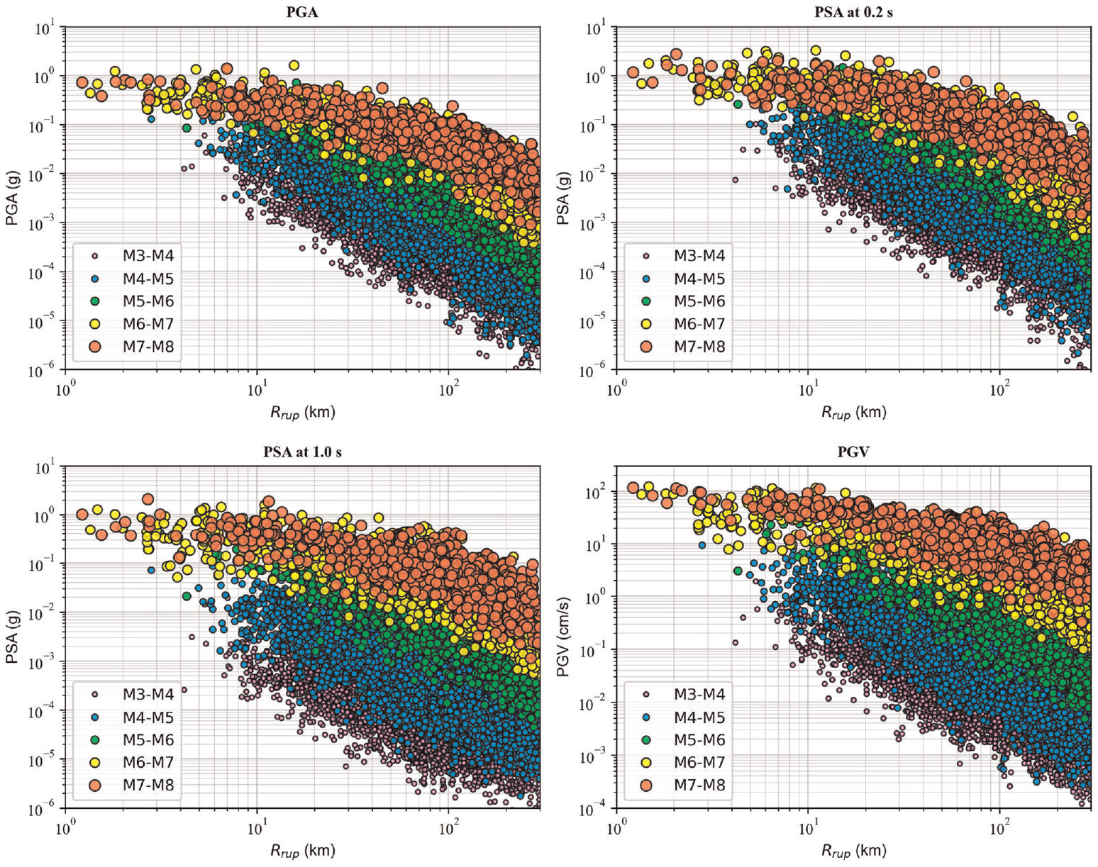
Magnitude and distance dependence of PGA, PSA at 0.2 s, PSA at 1.0 s, and PGV.

Data preparation

We use moment magnitude (M, unitless), rupture distance (closest three-dimensional distance to the rupture plane R_rup, in km), depth to the top of the rupture plane (Z_TOR, in km), and time-averaged shear wave velocity in the upper 30 m (V_S₃₀, m/s) as input parameters to the ML models. These parameters account for the magnitude, distance, depth, and site response scaling, respectively. The outputs or target values are defined as the natural logarithm of the RotD50 horizontal component of PGA (in units of g), 5%-damped PSA (in g) at different periods, PGV (cm/s), and PGD (cm). An initial explanatory data analysis of the recorded ground motions shows that the logarithm of GMIMs can be captured better with the logarithm of R_rup and V_S₃₀. Due to this observation and the high positive skewness of these input variables, R_rup and V_S₃₀ are transformed using a natural logarithmic function. The following equations represent the input and output matrices X and Y, respectively:

X = [\begin{matrix} M & l n (R_{r u p}) & Z_{T O R} & l n (V_{S 30}) \end{matrix}]

(1)

Y = [\begin{matrix} \ln (PGA) \begin{matrix} \ln (PS A_{0.01 s}) \dots \end{matrix} \begin{matrix} \ln (PGV) \ln (PGD) \end{matrix} \end{matrix}]

(2)

Input parameters are continuous and therefore are considered numerical features. ML algorithms, except for tree-based models, are sensitive to unscaled numerical features, and the process of training can be extremely slow if unscaled data are fed to these algorithms. Furthermore, many gradient-based estimators are designed to work with normalized or standardized data with values close to 0; therefore, using unscaled data can prevent convergence (Brownlee, 2016a). In this regard, we normalize each input parameter to the range of [0,1] to be fed to the ML algorithm without changing the distribution of the features. The normalization process for a given value in the input vector can be done by subtracting the minimum value from that given value and dividing the result by the difference between the maximum and minimum values.

Note that “region” is one of the additional explanatory variables in the NGA-West2 GMMs (except for Idriss, 2014) to allow for regionalization of the V_S₃₀ scaling and the anelastic attenuation (i.e. Q-term). The final data set includes 285 earthquakes, 265 of which occurred in California, 2 in Alaska, 1 in Nevada, 2 in Iran, 5 in Italy, 3 in Japan, 2 in New Zealand, 1 in Taiwan, 2 in Turkey, 1 in Georgia, and 1 in Montenegro. Including adjustment factors for the path and site terms in the functional form is straightforward. However, the inclusion of region as an explanatory variable (a categorical feature) in ML algorithms results in dividing the data set into various parts, and since more than 90% of earthquakes are from California, the final model will not be robust for other regions. Thus, the proposed GMMs are global, and the user based on the region of interest may require performing some post-processing steps to account for systematic differences in site and path effects, such as the hybrid empirical approach of Campbell (2003) and Pezeshk et al. (2018) or the referenced empirical approach of Atkinson (2008, 2010) based on the use of residual analysis. Another explanatory variable in the NGA-West2 GMMs is sediment thickness via Z_1.0 or Z_2.5 value, the depth to the 1 or 2.5 km/s shear wave velocity horizon beneath the site, respectively, to account for the de/amplification of deep sediment sites. This information is available through measurements or simulations for Japan and several California sites (Ancheta et al., 2014). Sediment depth is a numerical feature, and it is required to fix unknown values before feeding the numerical feature into ML algorithms. In this regard, all the earthquakes in other countries and also some California earthquakes with an unknown sediment depth should be removed, or the sediment depth should be imputed from other methods, such as using a median or mean value. There are some equations to evaluate the sediment depth using V_S₃₀ for Japan and California (Campbell and Bozorgnia, 2014; Chiou and Youngs, 2014). However, using these equations to compute the unknown sediment depths causes multicollinearity in ML algorithms. Therefore, we have not included the basin depth as an input parameter. We also chose to drop the style-of-faulting term from the explanatory variables list. In the final data set, the number of earthquakes with strike-slip, normal, and reverse mechanisms are 198, 25, and 62, respectively. All NGA-West2 GMMs include the style-of-faulting terms in their function form. However, the final regression results of Boore et al. (2014), Abrahamson et al. (2014), and Campbell and Bozorgnia (2014) GMMs are such that there is no scaling between strike-slip and reverse events. Abrahamson et al. (2014) explained that the Z_TOR term instead accounts for the scaling of reverse events due to the correlation between style-of-faulting and Z_TOR in the NGA-West2 data set. Chiou and Youngs (2014) also mentioned that the style-of-faulting effect is weaker for M < 6 earthquakes. We initially included this term in our analysis but found the term statistically insignificant, and thus, in the final version of the model, we dropped the style-of-faulting term. Similar trends have been observed in other regions, such as Europe and the Middle East (Kotha et al., 2016, 2020) and Iran (Sedaghati and Pezeshk, 2017).

Each ML algorithm, in addition to explanatory variables, has several input parameters, known as hyperparameters, that control the learning process. These hyperparameters are chosen by the user and are fixed during the training process and are passed as arguments to the constructor of the estimator. Note that hyperparameters are different from the regular parameters of ML methods, such as weights or coefficients that are derived from training. The process of selecting a set of optimal hyperparameters for an ML algorithm is called hyperparameter optimization or tuning. Grid search is a traditional way of the hyperparameters tuning process, which is an exhaustive search through a predefined subset of the ML method’s hyperparameters space. After defining the range of feasible values for all hyperparameters, we build a model for each possible combination of all hyperparameter values provided and measure the model’s performance using the loss function. Hyperparameter tuning finds a set of hyperparameters that results in an optimal model which minimizes a predefined loss function on a given test data set.

Note that if we use the same training data for evaluating the selected model, there is a chance of overfitting, and then the model can be failed and results in high errors for unseen data because ML algorithms are able to memorize the data instead of learning a generalized pattern if a bad set of hyperparameters are chosen (Brownlee, 2016b; Kuhn and Johnson, 2013). To perform the hyperparameter tuning process, we use a standard procedure called k-fold cross-validation (CV) (Brownlee, 2018; Kuhn and Johnson, 2013; Stone, 1974). In this regard, we first separate a test set from the selected final data set to use for the final evaluation of our models. The remaining data are then split into k number of folds (subsets). The CV process iterates through the k − 1 subsets and uses the hold-out subset at each iteration for validation. This process is repeated until every subset has been used as a validation set. Then, the average loss value is reported as the performance metric. A single run of the k-fold CV approach may lead to a noisy prediction of the model performance since different splits of the data result in various results. One solution to decrease the noise in the model performance is to increase the k-value. This will reduce the bias in the model performance; however, it will increase the variance.

An alternative method is to repeat the k-fold CV process multiple times and report the mean performance over all subsets and all repeats. This approach is referred to as repeated k-fold CV (Brownlee, 2020; Kuhn and Johnson, 2013). We partitioned the final subset into two different sets, 80% for training and validation using a tenfold CV procedure with three repetitions and 20% for testing to evaluate the performances of different models in estimating GMIMs using unseen test data. We use a stratified split method to keep the distributions of explanatory variables in the training and testing data sets the same as the entire data set.

Individual ML models

The GMIM estimation is treated as a regression problem, and the GMM can be expressed as

\ln (GMIM) = f [M, \ln (R_{rup}), Z_{TOR}, \ln (V_{S 30})] + ε

(3)

in which ln(GMIM) is the natural logarithm of the RotD50 horizontal GMIM of interest (PGD in cm, PGV in cm/s, and PGA and 5%-damped PSAs in g unit), function f gives the estimated GMIMs in natural log units, and ε is the residual (aleatory variability) representing the random variability of data relative to the model. A positive residual indicates that the model underpredicts the observation and a negative residual indicates that the model overestimates the observation. To perform a fully data-driven modeling process, we use four well-established supervised nonparametric ML algorithms, including ANN, KRR, RFR, and SVR to construct predictive GMMs. There are several researchers who have used ANN (Ahumada et al., 2015; Alavi and Gandomi, 2011; Derras et al., 2012, 2014; Dhanya and Raghukanth, 2018; García et al., 2007; Gök and Kaftan, 2022; Güllü, 2012; Khosravikia and Clayton, 2021; Khosravikia et al., 2019; Sedaghati et al., 2009; Sreenath et al., 2023; Vemula et al., 2023) or RFR (Khosravikia and Clayton, 2021; Kong et al., 2019; Kubo et al., 2020; Sreenath et al., 2023), or SVR (Hu and Zhang, 2022; Khosravikia and Clayton, 2021; Sreenath et al., 2023; Tezcan and Cheng, 2012) to develop GMMs for different regions; however, our study is the first to use a KRR approach to develop GMMs.

The detailed process of model construction and hyperparameters’ tuning can be found in the Supplementary material. The final selected ANN has two layers having eight and four nodes in the first and second layers, respectively, and tanh as the activation function in hidden layers and a linear activation function for the output layer. We used the Adam optimizer with a batch size of 128. The KRR model has a Gaussian kernel with alpha and gamma equal to 1 as the regularization strength and radial basis function (RBF) parameters, respectively. The selected RFR model uses a bootstrap resampling using 90% of the total training data and the minimum number of samples required at the leaf node and the minimum number of samples for a split at each node are set to 6 and 10, respectively. The final SVR model has a Gaussian kernel and C, gamma, and epsilon values indicating regularization parameter which controls the trade-off between maximizing the margin and minimizing the error, kernel coefficient, and penalty distance threshold, respectively, are set to 15, 0.01, and 0.1, respectively.

It should be noted that ANN natively supports multitarget regression; however, KRR, RFR, and SVR can predict a single target only at a time; thus, the regressor should be fitted separately for each period. An initial analysis of ANN showed us that the multitarget regression results in biased residuals for different periods since the network is fitted for all periods at once, mixing the correlation between different periods. Thus, even for the ANN model, we use one target at a time to solve for the weights and biases of the network. We use the MultiOutputRegressor strategy in Python from the “sklearn” package to feed the entire target variables mentioned in Equation 2 into the model and solve the regression by fitting one regressor per target. Because we use a repeated tenfold CV procedure with three repetitions, for each set of hyperparameters, 30 different models are fitted and evaluated. A mean squared error (MSE) is considered the model performance metric (score), and the best set of hyperparameters is the one having the lowest MSE. When several hyperparameter combinations result in nearly similar MSE values, the model with the lowest Bayesian information criterion, BIC value (Schwarz, 1978), is selected, which can be obtained from

BIC = \log (\frac{SSE}{n - k}) + (\frac{k}{n}) \log (n)

(4)

where k is the number of training parameters, n is the available training samples, and SSE is the sum of squared errors for the training.

MSE, mean absolute error (MAE), and coefficient of determination (R²) using the difference between the test data and the predicted values (in ln scale) are used to evaluate the model performance. Generally, lower MSE and MAE values indicate better performance and lower variance. A higher R² value suggests a stronger correlation between independent and dependent variables with a maximum of R² = 1 in the case of a linear relationship. Table 1 lists the MSE, MAE, and R² values obtained from the test data using different ML algorithms with their optimal hyperparameters selected using a grid search and performance comparison using a tenfold CV procedure with three repetitions.

Table 1.

Performance of the different models on the testing data

Models	MSE	MAE	R ²
ANN	0.6350	0.6297	0.8799
KRR	0.6439	0.6328	0.8768
RFR	0.5247	0.5599	0.9026
SVR	0.6472	0.6351	0.8759
Ensemble	0.5818	0.5994	0.8891

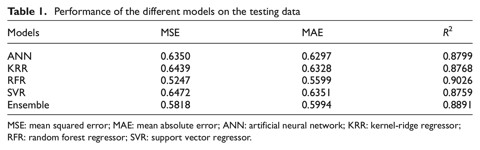
MSE: mean squared error; MAE: mean absolute error; ANN: artificial neural network; KRR: kernel-ridge regressor; RFR: random forest regressor; SVR: support vector regressor.

Ensemble model (weighted average)

Now, the question is how to select the best model among these models. The answer is that it is very subjective, and the results can be changed based on a given unseen data set. In addition, each method has several benefits while having some drawbacks. For instance, RFRs cannot extrapolate beyond the training data set, while ANNs can often perform well in the case of extrapolation. Of course, it is not guaranteed that ANN extrapolation follows precisely what we expect, but based on the trend in the training data, it can try to extrapolate for values outside the range of the training data. Note that RFRs report constant values similar to the boundary for values outside the training range. SVRs work well with high-dimensional data, and KRRs can perform better when there is multicollinearity in data compared to other approaches. In addition, the prediction from RFR is jagged, and the prediction from ANN is smooth.

To keep all advantages and remove the disadvantages of individual models, we can combine the outputs of several ML algorithms without the need to choose a model specifically. This process is called ensemble modeling (Raschka, 2018). The performance of the ensemble model is usually close to the best model for the training data, and sometimes it can outperform the performance of each model for unseen data. In the final data set, the data are sparse for the close distance range (less than 10 km), and even though the hyperparameters are selected to avoid overfitting, we may still observe large deviations among predictions from different ML models. By ensemble modeling for future events, we can effectively reduce the risk of an unfortunate selection of one poor model and improve predictions. Since we have selected the optimal hyperparameters for each regressor using a repeated tenfold CV technique, we train each model using the entire data set with the selected hyperparameters. Then, the results from all four supervised ML models are averaged using equal weights (1/4) to compute the final output. Hence, the contribution of each ML model to the ensemble model is equal (25%) for all ranges of explanatory variables. This is similar to using a logic tree approach in USGS national seismic hazard maps (Petersen et al., 2015). Furthermore, by weighted average ensemble modeling, the model-to-model epistemic uncertainty associated with the predictions due to the limitation of individual models is captured (Sreenath et al., 2023). A similar approach has been used by Sreenath et al. (2023), in which they developed ensemble GMMs for the Pan-European strong motion data set using five nonparametric ML models: shallow neural network, deep neural network, gated recurrent unit, support vector, and random forest regression. Based on the performance of individual ML models, all models have similar performance metrics; therefore, it is reasonable to use equal weights. All individual models are provided as Supplementary material, and definitely, one can change the weights within different magnitude–distance ranges based on additional criteria.

Figure 3 compares the distance scaling for PGA determined from the weighted average ensemble model with the individual ML algorithms for M4.5 and M7.5 events with a Z_TOR = 5 km and V_S₃₀ = 400 m/s. There is a significant variation between different ML algorithms for the distance range of less than 10 km; however, the number of records increases with increasing distance, resulting in more robust ML models with less variation. Moreover, as explained, RFR results in jagged curves and cannot extrapolate beyond the training input parameters range, particularly for M4.5, where there are no data with distances less than 8 km. This justifies using equal weights for different ML models even though the RFR model has the lowest MSE on the test data set. Figure 4 compares the response spectra predicted from the ensemble model with the individual ML algorithms for an M6.5 with a Z_TOR = 10 km and V_S₃₀ = 400 m/s at rupture distances of 35 and 100 km. As can be seen, the average curve is smooth in the middle of all estimators. At a rupture distance of 35 km, the ensemble model is very similar to the ANN model; however, at a rupture distance of 100 km, the ANN model predicts larger amplitudes compared to other models and the ensemble model is closer to KRR and SVR models. In both cases, the RFR curve is lower compared to other regressors.

Figure 3.

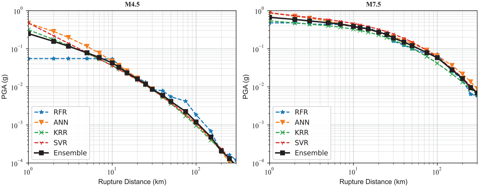
PGA distance scaling obtained from the individual ML algorithms versus the ensemble model for M4.5 (left) and M7.5 (right) events with a Z_TOR = 5 km and V_S₃₀ = 400 m/s.

Figure 4.

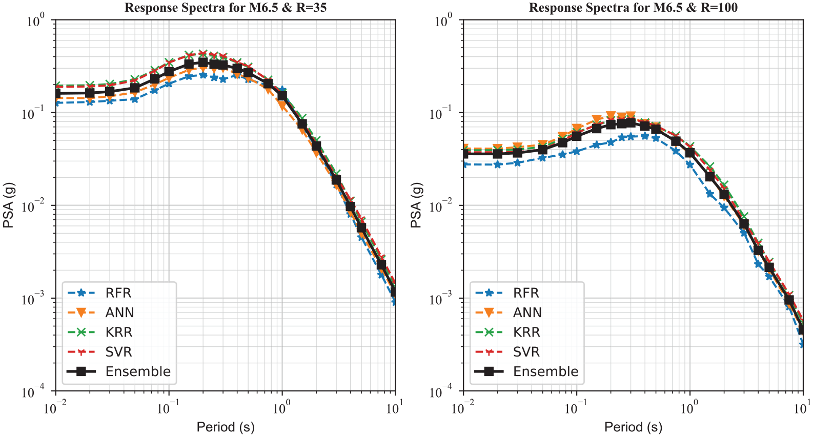
Response spectra predicted from the individual ML algorithms versus the ensemble model for an M6.5 event with a Z_TOR = 10 km and V_S₃₀ = 400 m/s at rupture distances of 35 and 100 km.

As listed in Table 1, the performance of the weighted average ensemble model is better than ANN, KRR, and SVR. Although the performance of the weighted average ensemble model does not beat RFR, the predictions are not jagged like RFR (see Figures 3 and 4). A lower performance metric does not necessarily mean that the model is the best for predicting new data, specifically where no or limited data were available for training. Note that these values are obtained using the test data set, and in the following section, we will show that for some recently recorded ground motions, the performance of those ML models compared to the ensemble model can change for unseen data. This indicates that until the data are limited in some ranges of the magnitude–distance space, ensemble modeling of ML models outperforms individual ML models for the entire range of magnitude, distance, and period.

Figure 5 shows the decay rate (attenuation) of the predicated spectral accelerations at different periods of 0, 0.2, and 1.0 s and PGV with distance for events with a Z_TOR = 0 km and V_S₃₀ = 760 m/s. Although the ensemble model is obtained from entirely data-driven ML algorithms, the model can capture the saturation effects, and for distances less than 10 km, M6.5, and M7.5 curves merge and result in similar GMIMs. In addition, the effect of geometrical spreading at shorter distances and anelastic attenuation at longer distances can be observed particularly for higher magnitudes. Moreover, the magnitude-dependent hinge point at which the slope of the decay rate is changed can be captured by ML algorithms. One interesting point from the distance scaling curves is the existence of oversaturation resulting in GMIM decreases with increasing M at very close distances. We observed that GMIMs from M7.5 at distances less than 5 km can be 3%–7% less than GMIMs from M6.5 at short periods up to 0.3 s. This pattern is seen in the NGA-West2 GMMs. Abrahamson et al. (2014) (see Figure 8) explained that the crossing of the M7.0 and M8.0 curves is due to the Z_TOR scaling. In fact, it is expected to have larger Z_TOR values with decreasing M; thus, M8 with Z_TOR = 0 can be compared with M7 with Z_TOR larger than 0; however, in our plot, we used a constant Z_TOR of 0 km for all magnitudes.

Figure 5.

Distance scaling characteristics of the developed ensemble GMMs for events with a Z_TOR = 0 km and V_S₃₀ = 760 m/s for PGA, PSA at 0.2 s, PSA at 1.0 s, and PGV.

Boore et al. (2014) (see Figure 6) mentioned that, unlike their previous version of GMMs, they did not constrain the oversaturation term because some simulations support oversaturation (Schmedes and Archuleta, 2008). Our suite of GMMs is purely data-driven with no constraints; therefore, as can be suggested from observed ground motions in Figure 2, oversaturation can occur. It is worth mentioning that the NGA-West2 GMMs consider an additional parameter, fictitious depth obtained during the regression process, to calculate the effective distance; however, our GMMs do not have any fictitious depth defined. As Boore (2009) and Tavakoli et al. (2018) discussed, although larger magnitude earthquakes have higher energy, they have larger finite-fault dimensions resulting contribution of energy from grid cells on the fault that are much further away. Therefore, they suggest using effective distance from the fault instead of regular distance metrics such as rupture distance to account for the fault dimension. Calculation of the effective distance for a given earthquake requires detailed information of the fault and the source-to-site direction (Tavakoli et al., 2018), which is beyond the scope of this article.

Figure 6.

Variation of estimates of response spectra versus spectral period for events with a Z_TOR = 0 km and V_S₃₀ = 400 m/s at rupture distances of 35 and 100 km.

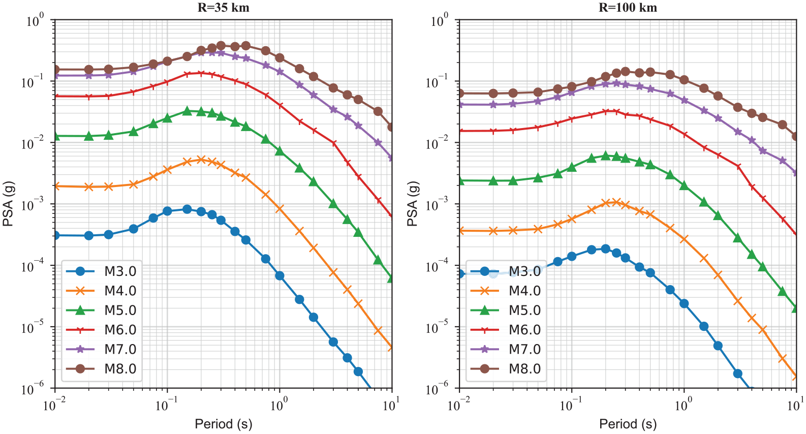
Figure 6 illustrates the variation of estimates of response spectra versus spectral period for events with a Z_TOR = 0 km and V_S₃₀ = 400 m/s at rupture distances of 35 and 100 km. As can be seen, the gap between curves is decreased by increasing the magnitude, and for shorter distances, this reduction is more, and M7 and M8 at a rupture distance of 35 are close, indicating the saturation effects. Furthermore, it can be observed that the period corresponding to the maximum amplitude shifts toward higher periods with an increasing magnitude which Boore et al. (2014) call the M-dependence of the predominant period. These observations are similar to the NGA-West2 GMMs (Abrahamson et al., 2014; Boore et al., 2014; Campbell and Bozorgnia, 2014; Chiou and Youngs, 2014; Idriss, 2014).

Epistemic uncertainty

Epistemic uncertainty refers to the uncertainty arising from a lack of knowledge or understanding of a phenomenon or process due to sparse data, limitations in the mathematical equations or ML algorithm used to model ground motion, and/or differences in assumptions and interpretations of the available data. For instance, GMMs are constructed based on the data available, and if the data are sparse, the predictions made by the model may not be entirely accurate. To capture this epistemic uncertainty, known as model-to-model variability, we will compute the deviation in all four models from the ensemble model (Atik and Youngs, 2014; Sreenath and Raghukanth, 2023; Sreenath et al., 2023).

Figure 7 depicts the epistemic uncertainty for the distance scaling of PGA and PGD for M5 and M7 events with a Z_TOR = 5 km and V_S₃₀ = 400 m/s. The band represents the model-to-model variability as mean ± sigma, defined as the deviation in all four models from the weighted average ensemble model. Furthermore, the observed ground motions are plotted for comparison. The comparison of the model-to-model variability with the observed ground motions shows that magnitude–distance ranges with a large number of recorded data have lower epistemic uncertainty indicating all four ML models predict similar GMIMs. However, magnitude–distance ranges with inadequate or no data, particularly for distances less than 10 km, have higher epistemic uncertainty meaning that using just one ML algorithm can be unreliable in predicting GMIMs for a future event while using an ensemble model can avoid this. Sreenath et al. (2023) had a similar observation developing ensemble GMMs for the Pan-European strong motion data set using five nonparametric ML models.

Figure 7.

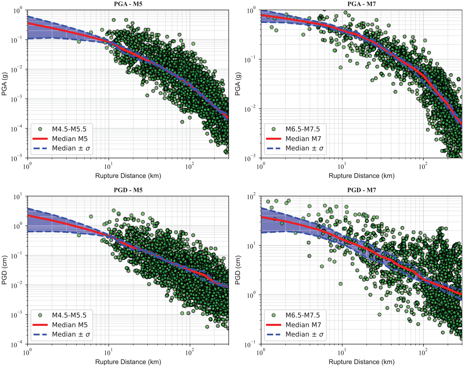
Epistemic uncertainty for the distance scaling of PGA and PGD for M5 and M7 events with a Z_TOR = 5 km and V_S₃₀ = 400 m/s. The band represents the model-to-model variability as mean ± sigma defined as the deviation in all four models from the ensemble model.

Aleatory uncertainty

The total residual can be partitioned into between-event, between-station, and event-site–corrected residuals (Atik and Abrahamson, 2010) using different techniques such as two-stage regression or mixed-effects regression methods (Kotha et al., 2016; Rodriguez-Marek et al., 2014; Sedaghati and Pezeshk, 2016; Stafford, 2014). The between-event, between-station (site-to-site), and event-site–corrected residuals are assumed to be independent, normally distributed with a zero mean and standard deviation of τ, $ϕ_{S 2 S}$ , and $ϕ_{SS}$ , respectively (Atik and Abrahamson, 2010). To perform site-specific PSHA, the single station standard deviation can be defined as

σ_{SS} = \sqrt{τ^{2} + {ϕ_{SS}}^{2}}

(5)

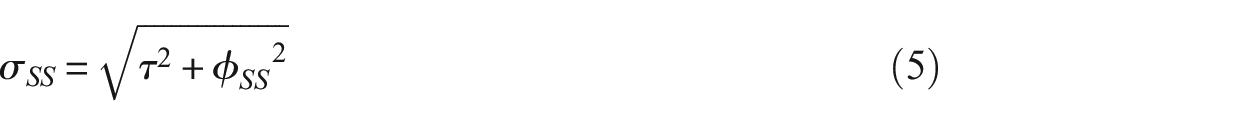
For traditional PSHA with ergodic assumptions, all residual components are used to obtain the total aleatory variability as

σ = \sqrt{τ^{2} + {ϕ_{SS}}^{2} + {ϕ_{S 2 S}}^{2}}

(6)

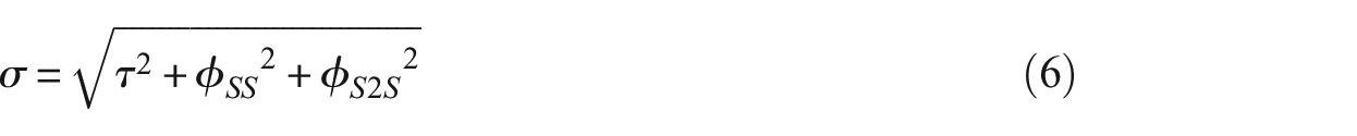
Since the selected data set has 1098 single-recorded stations and 477 stations with only 2 recordings, the inclusion of the between-station uncertainty lacks a logical and statistical basis and results in a biased estimation. Therefore, we compute the standard deviations in two stages. In the first stage, we use all recordings in the data set to split the total residuals into between-event and within-event components using a mixed-effects regression. Then, we remove stations with less than or equal to four records per station and create another data set with 11,513 recordings. This data set has recordings captured by at least five stations and stations recorded at least five earthquakes. The reduced data set is used to split the within-event residuals into between-station and event-site–corrected components in the second stage using another mixed-effects regression. The distribution of between-event residuals versus moment magnitude and the distribution of event-site–corrected and site-to-site residuals versus rupture distance and V_S₃₀ for PGA and PSA at 0.2 and 1.0 s is shown in Figure 8. The ideal residual value is zero, indicating that the model accurately estimates the target value. Overall, the residuals are centered around zero with no trends and no obvious biases, with M, R_rup, and V_S₃₀ indicating good agreement between the proposed model and observed ground motions.

Figure 8.

Distribution of between-event, between-station (site-to-site), and event-site–corrected residuals (in natural logarithm units) for PGA and PSA at spectral periods of 0.2 and 1.0 s. Error bars represent the mean and standard deviation of the binned residuals.

The variations of $τ$ , $ϕ$ , $ϕ_{S 2 S}$ , $ϕ_{S S}$ , and $σ$ versus period are presented in Table 2 and depicted in Figure 9. As can be seen, there is a bump near 0.075 s in both within-station and total standard deviations. This bump has been seen in some of the NGA-West2 models. Boore et al. (2014) suggested that two processes can contribute to this bump: (1) variation in the source stress parameter for small earthquakes particularly and (2) variation in κ₀ (near-source attenuation defined by the decay slope of the spectrum at high frequencies at near-source distances, Boore, 2003) for larger earthquakes.

Table 2.

Associated standard deviations of the ensemble GMMs in natural logarithm units

Periods	$σ$	$τ$	$ϕ$	$ϕ_{S 2 S}$	$ϕ_{SS}$
PGA	0.7276	0.3022	0.6509	0.4365	0.4828
0.01	0.7290	0.3032	0.6520	0.4378	0.4831
0.02	0.7318	0.3048	0.6543	0.4404	0.4840
0.03	0.7448	0.3141	0.6641	0.4522	0.4863
0.05	0.7827	0.3396	0.6934	0.4903	0.4902
0.075	0.8015	0.3499	0.7089	0.5101	0.4923
0.1	0.7970	0.3439	0.7070	0.4997	0.5000
0.15	0.7826	0.3203	0.7022	0.4928	0.5003
0.2	0.7673	0.3068	0.6918	0.4799	0.4983
0.25	0.7460	0.2947	0.6742	0.4530	0.4994
0.3	0.7311	0.2856	0.6622	0.4363	0.4981
0.4	0.7058	0.2828	0.6363	0.4179	0.4798
0.5	0.6969	0.2919	0.6225	0.4044	0.4733
0.75	0.6820	0.3140	0.5952	0.3921	0.4479
1	0.6850	0.3408	0.5840	0.3907	0.4340
1.5	0.6812	0.3554	0.5709	0.3767	0.4290
2	0.6753	0.3588	0.5621	0.3575	0.4337
3	0.6793	0.3632	0.5640	0.3401	0.4499
4	0.6772	0.3571	0.5653	0.3254	0.4623
5	0.6822	0.3583	0.5703	0.3186	0.4729
7.5	0.6918	0.3705	0.5739	0.3074	0.4846
10	0.6789	0.3651	0.5622	0.3016	0.4745
PGV	0.6439	0.2715	0.5744	0.3418	0.4616
PGD	0.6863	0.3727	0.5661	0.3072	0.4754

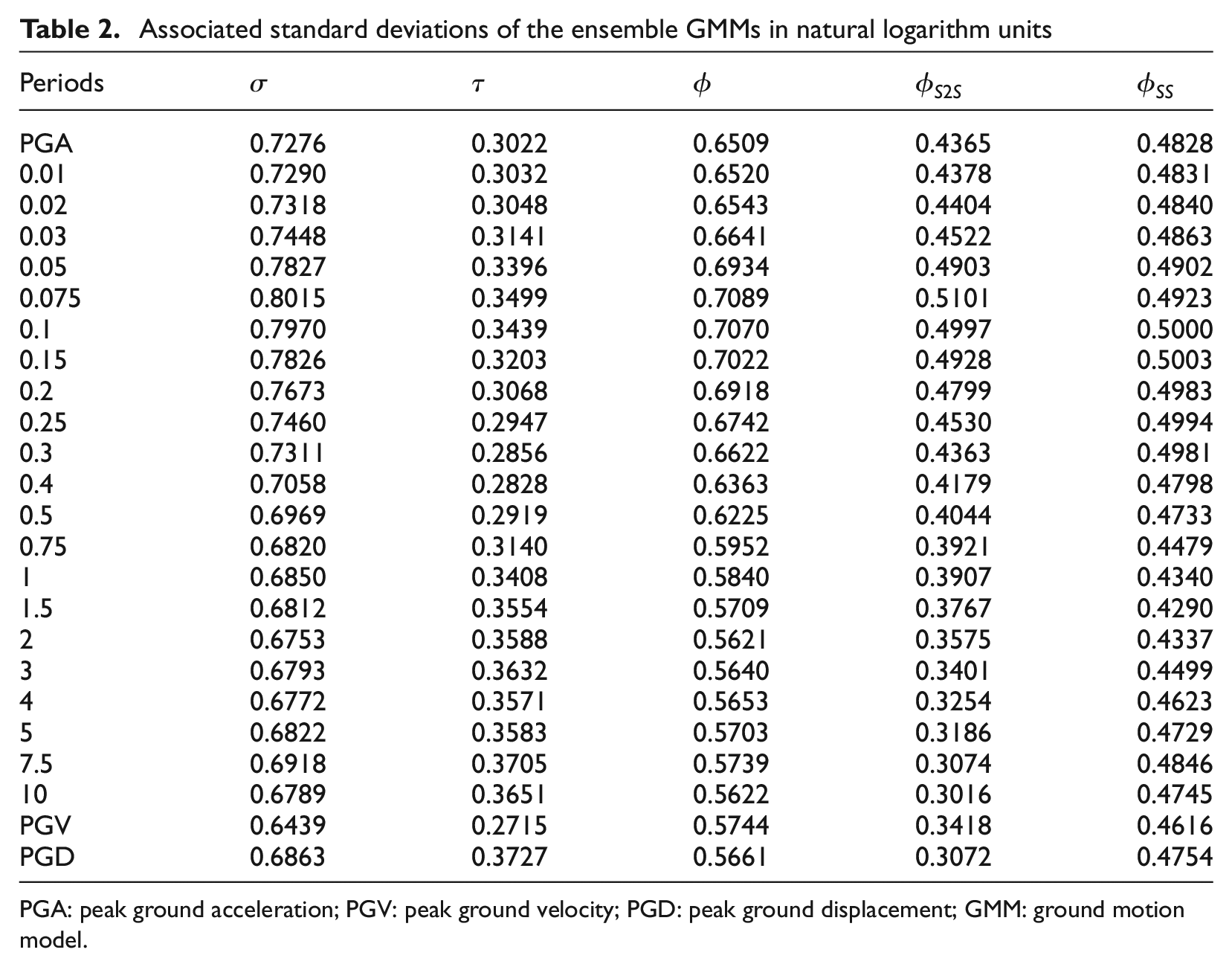
PGA: peak ground acceleration; PGV: peak ground velocity; PGD: peak ground displacement; GMM: ground motion model.

Figure 9.

Variation of different aleatory standard deviations versus spectral period.

Comparison with previous models developed for active shallow crustal regions

In this section, the final developed GMMs are compared with all five NGA-West2 GMMs: Abrahamson et al. (2014), Boore et al. (2014), Campbell and Bozorgnia (2014), Chiou and Youngs (2014), and Idriss (2014) referred to as ASK14, BSSA14, CB14, CY14, and I14, respectively.

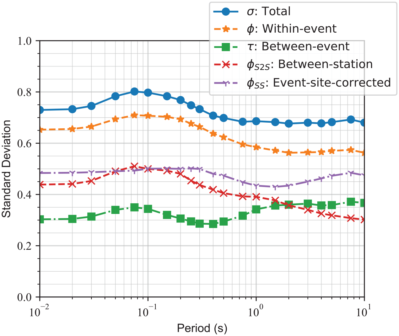
Figure 10 compares response spectra from our ensemble GMMs, SP23, with ASK14, BSSA14, CB14, CY14, and I14 GMMs. As can be seen, response spectra from our model are in good agreement with the NGA-West2 GMMs. We use a Z_TOR = 5 km and V_S₃₀ = 760 m/s for M5 and M7 events with rupture distances of 10 and 35 km. For lower magnitudes and shorter distances, our curve matches the CY14 model in the entire period range. For longer distances and lower magnitudes, SP23 is very close to the CY14 model in the shorter period range, while it is closer to the BSSA14 curve at the mid and longer period range. For the larger magnitudes, our GMMs predict slightly higher values, particularly in the mid-period range. We investigated this difference and found out that with decreasing Z_TOR for an M7 event, the gap between our ensemble model and the NGA-West2 GMMs in the middle period range becomes smaller. Overall, at short distances for larger magnitudes, our curve is very close to the CB14 model for the shorter period range, whereas, for long distances, it matches the ASK14 model in the shorter period range. For M7 and longer period range, our curve is in between the other NGA-West2 model.

Figure 10.

Comparison of the period-dependence of 5%-damped pseudo-spectral accelerations derived from the present model with the NGA-West2 GMMs for events with a Z_TOR = 5 km and V_S₃₀ = 760 m/s.

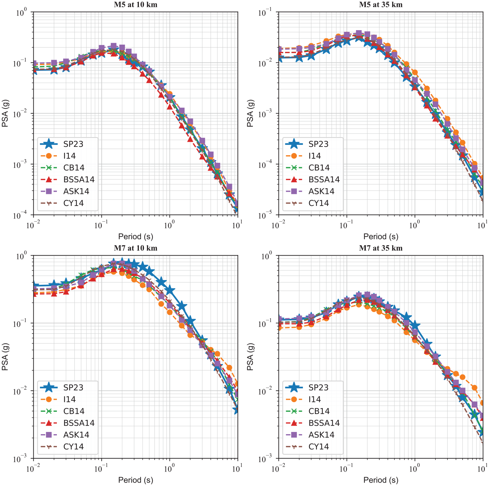
Figure 11 compares the magnitude scaling of our proposed GMMs, SP23, with ASK14, BSSA14, CB14, CY14, and I14 GMMs for PGA and PSA at 0.2, 1.0, and 5.0 s. We use a Z_TOR = 0 km and V_S₃₀ = 260 m/s for a rupture distance of 50 km. Some curves start at a larger magnitude since the applicable magnitude range for the CY14 and CB14 models is M4+, and for the I14 model is M5+. Generally, the magnitude scaling of our GMMs is consistent with the other NGA-West2 GMMs, and the curve is pretty close to CY14 for PGA and to ASK14 and BSSA14 for PSA at 0.2 s. For longer periods, all models result in a similar trend. As can be seen, the saturation effect from our GMMs is significant and comparable with the CB14 model, particularly for PGA and PSA at 0.2 s, while for longer periods, all models are similar.

Figure 11.

Comparison of the magnitude scaling of the estimated PSA values from the GMMs proposed in this study with the NGA-West2 GMMs at PGA as well as PSA at 0.2, 1.0, and 5.0 s at a rupture distance of 50 km for events with a Z_TOR = 0 km and V_S₃₀ = 260 m/s.

Figure 12 depicts the comparison of the V_S₃₀ scaling of our proposed GMMs, SP23, with ASK14, BSSA14, CB14, CY14, and I14 GMMs for PGA and PSA at 0.2 and 3 s. We use a Z_TOR = 1 km and M7 for rupture distances of 10 and 100 km. All GMMs are defined as a function V_S₃₀. Note that the I14 model should be used for V_S₃₀ ≥ 450 m/s. For the shorter-distance 10 km case, we can observe the curvature indicating the nonlinear site effects resulting in de-amplification. The nonlinear site effects are stronger for PSA at 0.2 s compared to PGA. The site amplification for the 100 km case is nearly linear with V_S₃₀ using all models. For PSA at 3 s, we can observe that all models have similar linear trend with V_S₃₀. Overall, the site response results are similar between the NGAWest2 models and our proposed GMMs, particularly in the range where there are a large amount of observed data. Based on this comparison, it is evident that the ML models can capture the linear and nonlinear site effects using V_S₃₀. It should be noted that the SP23 V_S₃₀ scaling curves are generally more jagged compared to the smooth NGA-West2 models because we have not used any simulated data and no prior function to perform curve fitting. This pattern is just observed by data and may be biased when there are not sufficient recorded ground motions for training.

Figure 12.

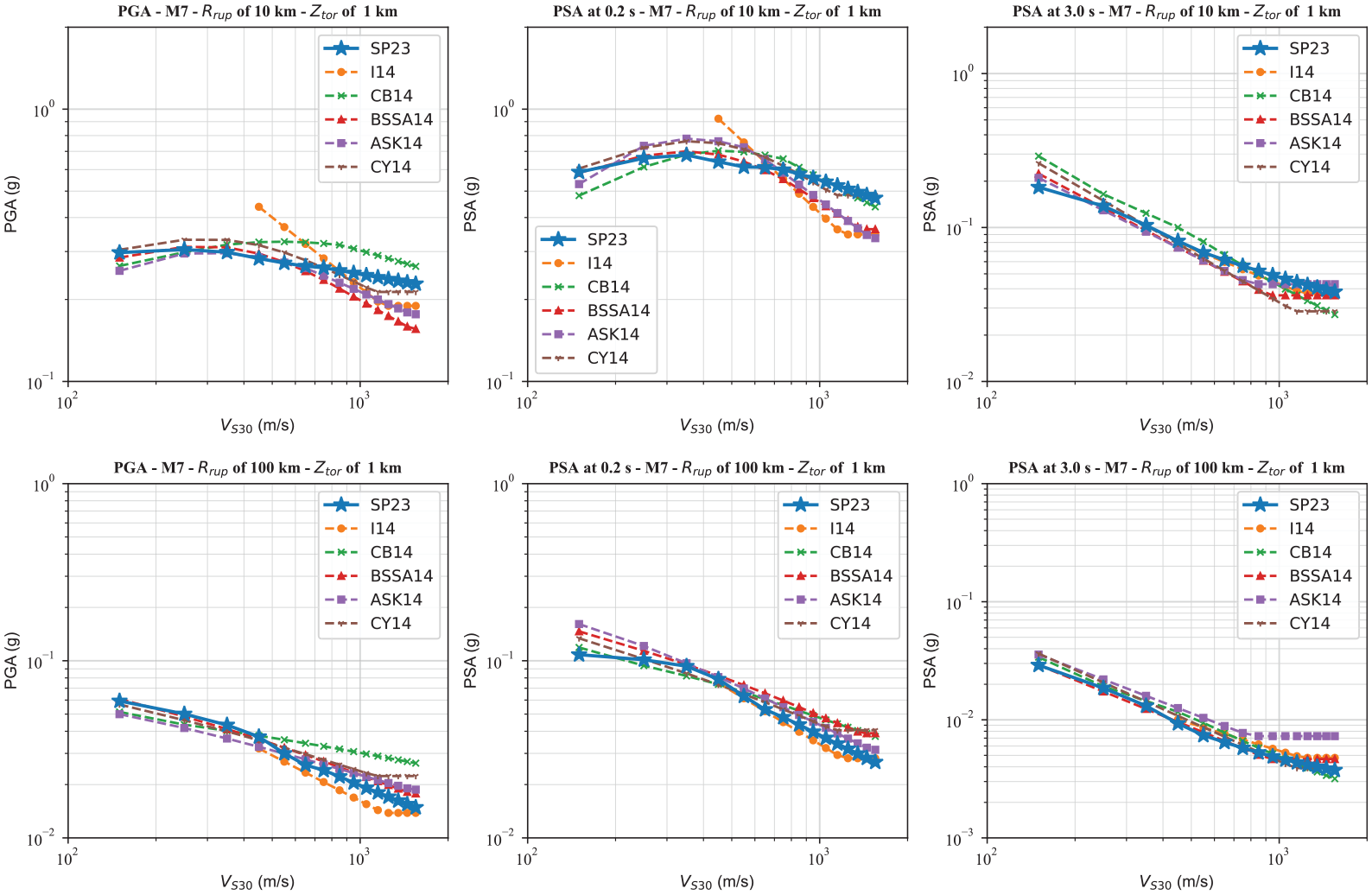
Comparison of the V_S₃₀ scaling of the estimated PSA values from the GMMs proposed in this study with the NGA-West2 GMMs at PGA and PSA at 0.2 at rupture distance of 10 (top) and 100 (bottom) km for events with M7 and a Z_TOR = 1 km.

The Z_TOR scaling of our proposed GMMs, SP23, with the NGA-West2 GMMs is compared in Figure 13. Z_TOR is not an input parameter for BSSA14 and I14. Also, default values used for other input parameters used in CB14 do not activate the Z_TOR scaling of the CB14 model. However, for comparison purposes, we plotted all NGA-West2 GMMs. We plotted Z_TOR up to 15 km for both M5 and M7 for visual purposes, but it should be noted that Z_TOR should be narrowing with increasing M (Abrahamson et al., 2014; Chiou and Youngs, 2014; Gregor et al., 2014). For the M5 case, the Z_TOR scaling of the ensemble model has a similar slope to ASK14 and CY14. It is interesting to note that the Z_TOR scaling of our GMMs and CY14 crosses the BSSA14 and CB14 Z_TOR scaling at Z_TOR of 5–7 km, which is the average depth to the rupture of M5 earthquakes in the NGA-West2 data set (Gregor et al., 2014). According to the equations provided by Abrahamson et al. (2014) and Campbell and Bozorgnia (2014), a bilinear function is used to determine the depth scaling factor. The hinge points for the depth scaling function are set at 10 and 16.66 km, respectively, for ASK14 and CB14. In this study, the ensemble GMMs exhibit more sudden changes in PGA and PSA. This could be attributed to a reduction in the number of events at greater depths or an increase in energy release for faults located deeper underground.

Figure 13.

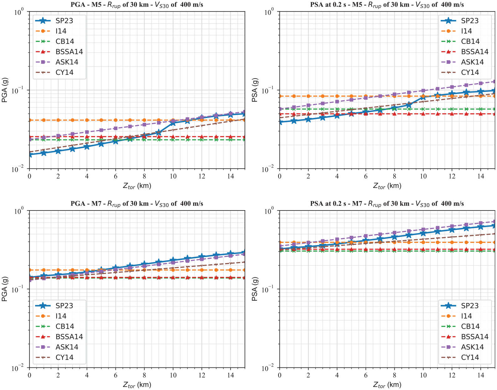
Comparison of the Z_TOR scaling of the estimated PSA values from the GMMs proposed in this study with the NGA-West2 GMMs at PGA and PSA at 0.2 at a rupture distance of 30 km for events with M5 and M7 and a V_S₃₀ = 400 m/s.

For M7 case, SP23, CY14, and ASK14 have a similar slope of the Z_TOR scaling. All ground motion values cross at Z_TOR of 0–2 km, which is the average depth to the rupture of M7 earthquakes in the NGA-West2 data set (Gregor et al., 2014). The ground motion value increases with increasing Z_TOR, confirming that buried ruptures are, on average, more energetic than events that rupture to the surface (Abrahamson et al., 2014).

Figure 14 compares the period dependence of the aleatory variability of the NGA-West2 GMMs with the ensemble GMMs. The NGA-West2 aleatory variability models are magnitude and distance-dependent, while we developed a magnitude and distance-independent aleatory variability. We plotted aleatory variability curves for a rupture distance of 50 km for M4, M5, M6, and M7. Generally, the shape of the total standard deviation of our model is similar to BSSA14 and CB14 aleatory variability models with a bump around 0.05–0.1 s and lower values at longer periods. For M4 and M5 cases, the total standard deviation from our model is lower compared to the total standard deviation values from the NGA-West2 models, whereas for M6 and M7, the total standard deviation of the model is larger for shorter periods (less than 1 s) and lower for longer periods (≥1 s) compared to the total standard deviation of the NGA-West2 models.

Figure 14.

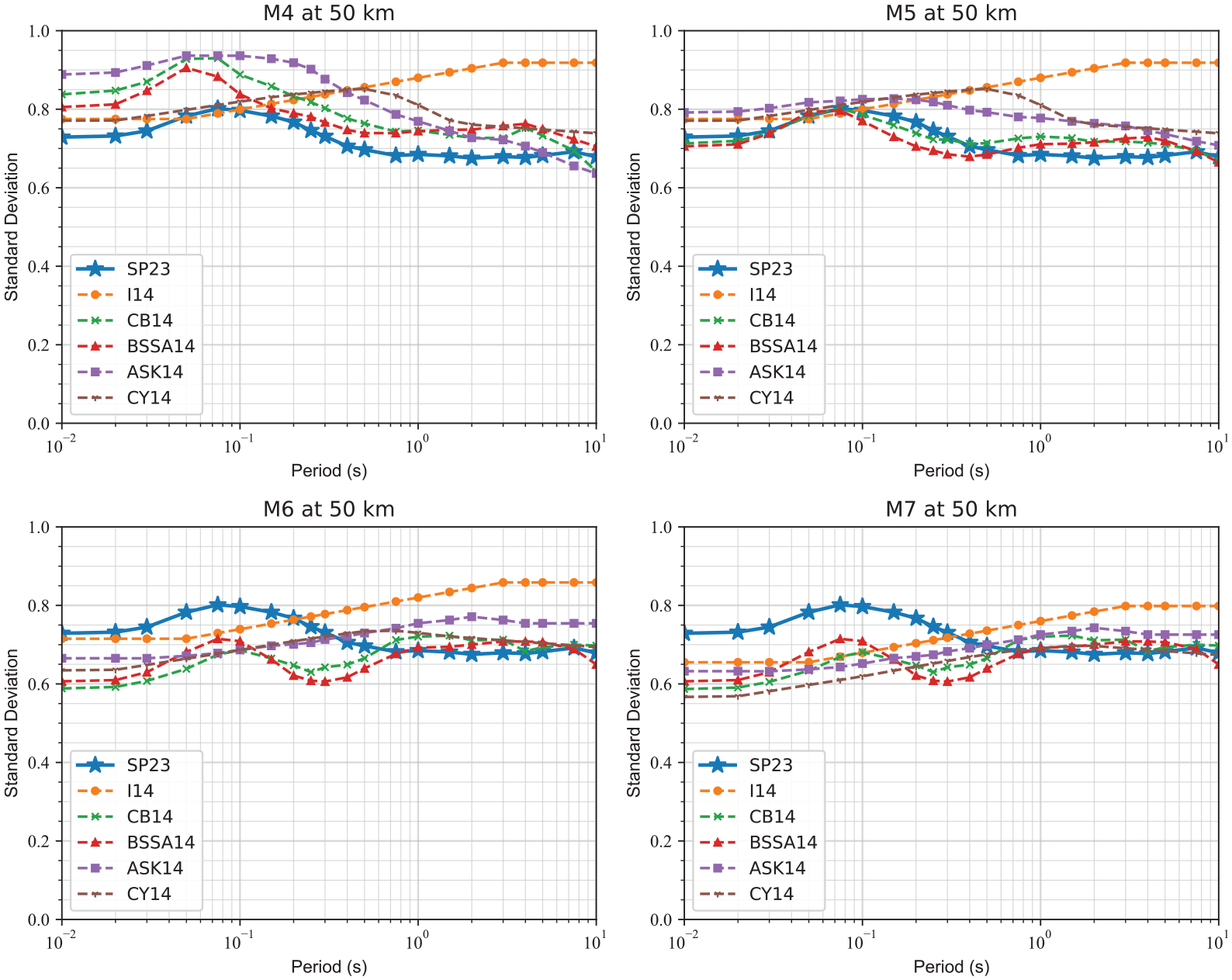
Comparison of the standard deviation from the GMMs proposed in this study with the NGA-West2 GMMs for events with magnitude 4, 5, 6, and 7 at a rupture distance of 50 km with a V_S₃₀ = 400 m/s.

Finally, for a true assessment of the predictive performance of the proposed GMMs in this study compared to the NGA-West2 GMM, we collect observed ground motions from two recent large earthquakes not included in the NGA-West2 database, the 2019 M7.1 Ridgecrest, California, and the 2023 M7.8 Turkey earthquakes. The details of these earthquakes and the recorded ground motions can be found on the USGS website (see section “Data and resources”). For the Ridgecrest earthquake, the RotD50 GMIMs are provided by Rekoske et al. (2019) and presented in detail in Rekoske et al. (2020) (see section “Data resources”). For the Turkey earthquake, we used the geometric mean of the two horizontal earthquakes, and we acknowledge that the results may change if the RotD50 GMIMs are used. The collected data set includes 250 and 763 observed ground motion recordings for the 2023 M7.8 Turkey and the 2019 M7.1 Ridgecrest earthquakes, respectively. The data set provides PGA and PSA at 0.3, 1, and 3 s. Figure 15 demonstrates the distance scaling of the ensemble and the NGA-West2 GMMs compared with observed ground motions for the 2023 M7.8 Turkey earthquake for PGA and PSA at 0.3, 1, and 3 s. For PGA, all NGA-West2 except for I14 have a similar performance. Note that all GMMs are applicable for rupture distances up to 300 (except for BSSA, which is applicable for distances up to 400 km), but we plotted the distance scaling up to 500 km to compare the extrapolation capability as well. We see some differences for PSA at 0.3, and our model has a similar trend to CB14 and BSSA14. For PSA at 1 s, all NGA-West2 models slightly underpredict at short distances, while our model predicts larger values than the NGA-West2 models. This trend can also be explained by the gap observed in Figure 10 between our ensemble model with the NGA-West2 GMMs. For PSA at 3 s, we can observe some differences at longer distances with slight underestimation from our model. Figure 16 illustrates the distance scaling of the ensemble and the NGA-West2 GMMs compared with observed ground motions for the 2019 M7.1 Ridgecrest earthquake for PGA and PSA at 0.3, 1, and 3 s. For PGA and PSA at 0.3 s, all models have reasonable and comparable performance. However, for PSA at 1 s, GMMs have a gap within the first 10 km, while this gap decreases with increasing distances. For PSA at 3 s, all models have a similar trend for distances larger than 10, while there is a significant variation for distances less than 10 km. This emphasizes that all GMMs with different functional forms or ML-based GMMs have comparable results for data-rich magnitude–distance ranges, whereas predications from various GMMs have considerable differences for magnitude–distance ranges with no or inadequate observed ground motions. We use MSE to numerically test the predictive power of the above-mentioned GMMs against the collected database. The resultant MSE values are tabulated in Table 3. For this analysis, we removed data with rupture distances greater than 300 km to have only data within the applicable range of all GMMs. Note that the full comparison of the performance of GMMs needs to use several popular approaches, such as the loglikelihood (LLH) method of Scherbaum et al. (2009) and its natural extension, known as the multivariate logarithmic score of Mak et al. (2017) or the Euclidean Distance–Based Ranking (EDR) of Kale and Akkar (2013). As presented in Table 3, the BSSA14 model is the best model with the lowest MSE for PGA for both earthquakes. For PSA at 0.3, 1, and 3 s, the SP23 model (weighted average ensemble model) outperforms the Turkey earthquakes, whereas the CY14 results in the lowest MSE for the Ridgecrest earthquake. This indicates that some models performed better in certain periods than others, and not a single model performed the best over the entire period range. Comparing the ensemble model with the individual ML models, we can recognize that ANN is the best model against the Turkey earthquake for PGA, SVR is the best model against the Ridgecrest earthquake for PGA, RFR has the lowest MSE against the Turkey earthquakes for PSA at 0.3 s, and for the rest of the cases, KRR outperforms the other ML models. KRR had not been used in the context of GMM development, and based on our study, this ML algorithm can be used to predict GMIMs for future earthquakes. Another interesting point is that even though RFR had the best performance on the test data set, the performance of this algorithm is not perfect on the collected data set, and at some periods, its MSE is twice the other ML models’ MSE values. Furthermore, it can be observed that the weighted average ensemble model beats all ML models against the Turkey earthquake for PSA at 0.3, 1, and 3 s and against the Ridgecrest earthquake for PGA and PSA at 0.3 s. This emphasizes that the weighted average ensemble model performs better over the entire range of M, R_rup, and period compared to the individual ML models. In addition to MSE values, MAE values, which are less sensitive to outliers, are provided in Table 3. A comparison of MAE values indicates that generally the SP23 (weighted average ensemble) model and CY14 perform better for all periods for Turkey and Ridgecrest earthquakes. Finally, it is worth mentioning that the suite of the CY14 GMM is a complex model compared to the other NGA-West2 GMMs with several input parameters and using many nonlinear functions inside its functional form, and our set of ML-based GMMs with only four input parameters without defining of any functional form can have a comparable performance. Note that since all models have been provided as the Supplementary material to this article, interested readers can use different GMM ranking schemes to assign different weight to each ML model using a given data set.

Figure 15.

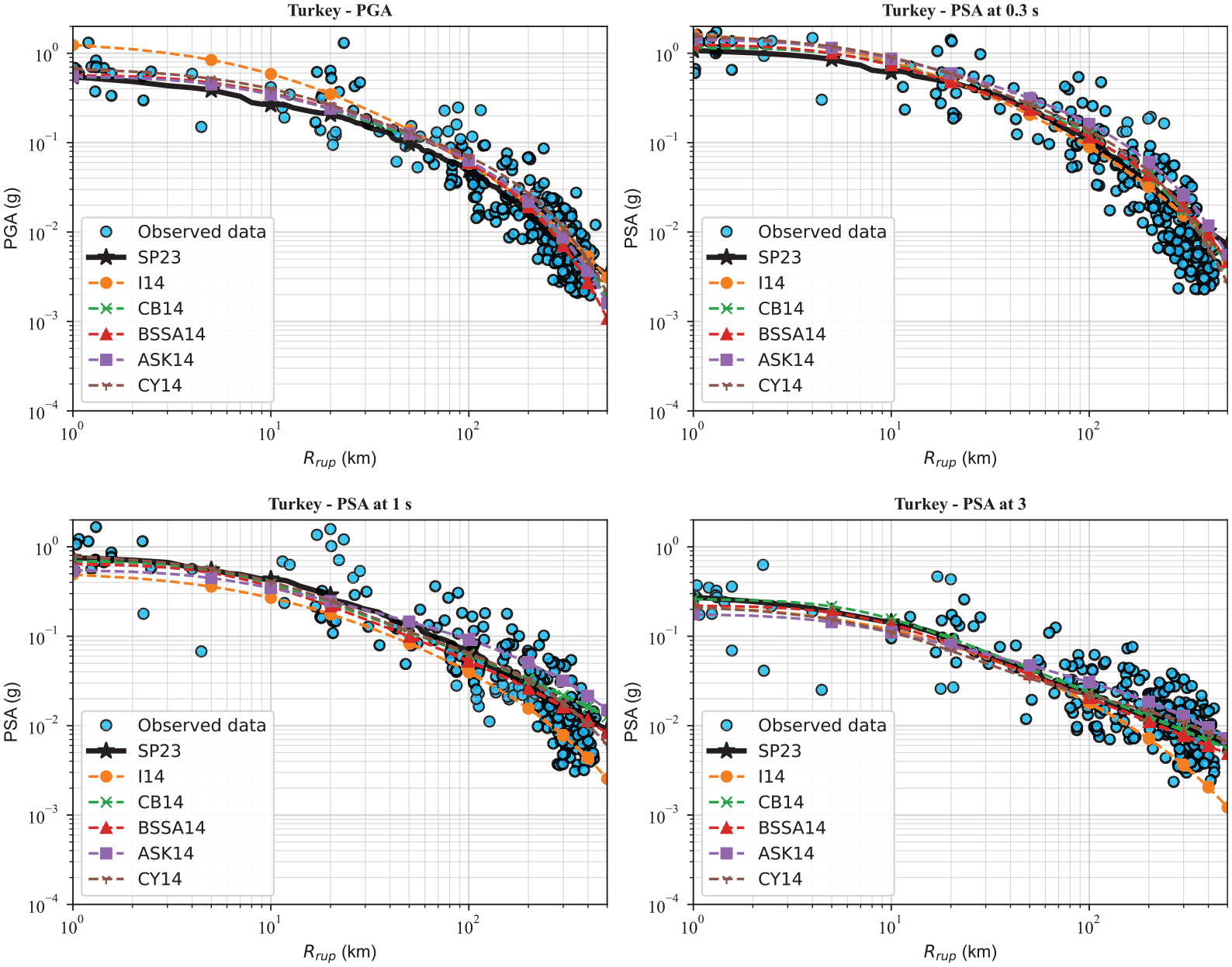
Assessing the predictive capability of NGA-West2 GMMs compared to the weighted average ensemble GMMs for the 2023 M7.8 Turkey earthquake.

Figure 16.

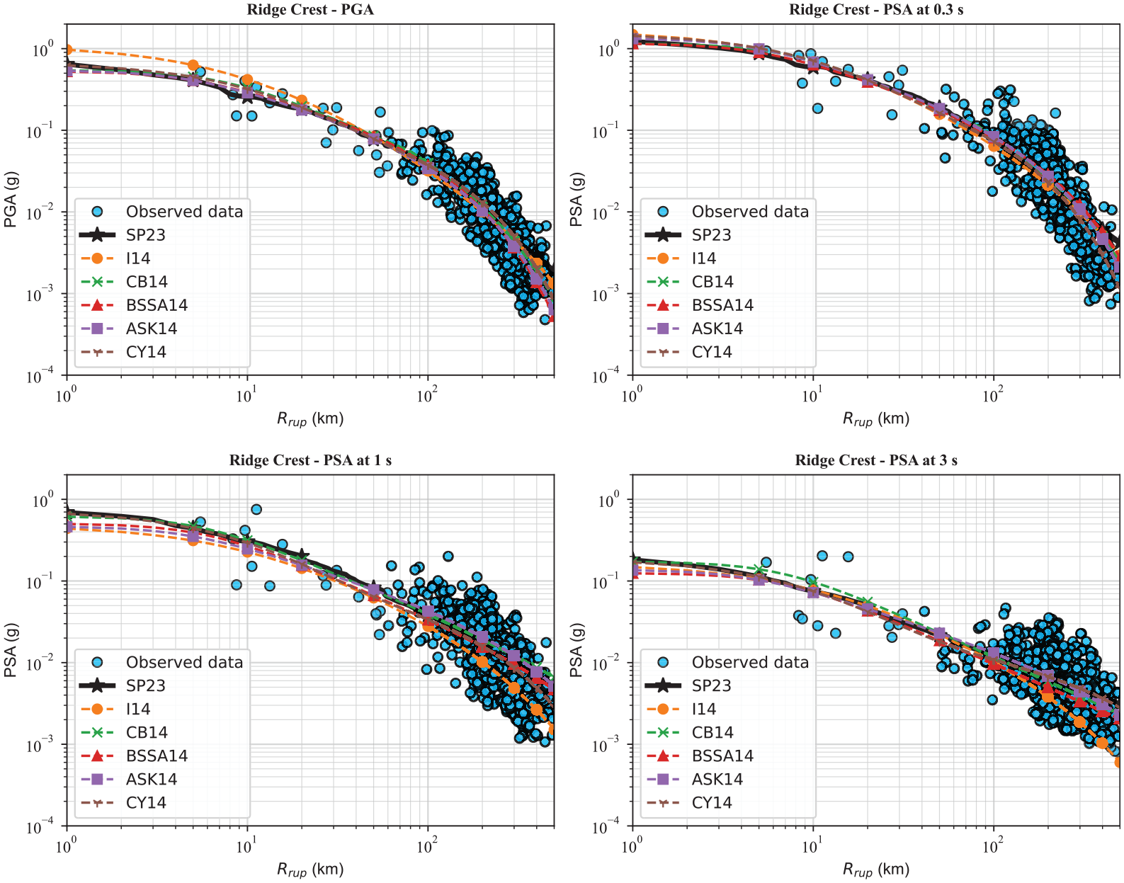
Assessing the predictive capability of NGA-West2 GMMs compared to the weighted average ensemble GMMs for the 2019 M7.1 Ridgecrest earthquake.

Table 3.

Performance of the different NGA-West2 and ML GMMs on the collected data set

Period	Earthquake	Metrics	I14	CB14	BSSA14	ASK14	CY14	SP23	ANN	KRR	RFR	SVR
PGA	Turkey	MSE	0.568	0.411	0.399	0.429	0.529	0.434	0.421	0.454	0.536	0.459
	Turkey	MAE	0.611	0.528	0.505	0.541	0.600	0.504	0.497	0.529	0.558	0.527
	Ridgecrest	MSE	0.244	0.261	0.229	0.246	0.259	0.232	0.238	0.246	0.317	0.238
	Ridgecrest	MAE	0.393	0.407	0.383	0.401	0.394	0.377	0.389	0.389	0.447	0.380
PSA at 0.3 s	Turkey	MSE	0.634	0.58	0.63	0.893	0.656	0.557	0.599	0.608	0.567	0.584
	Turkey	MAE	0.628	0.604	0.627	0.766	0.647	0.585	0.605	0.619	0.585	0.608
	Ridgecrest	MSE	0.374	0.343	0.362	0.348	0.333	0.35	0.414	0.364	0.391	0.367
	Ridgecrest	MAE	0.486	0.463	0.470	0.461	0.456	0.462	0.512	0.476	0.491	0.475
PSA at 1 s	Turkey	MSE	0.685	0.517	0.495	0.767	0.499	0.462	0.537	0.471	0.519	0.507
	Turkey	MAE	0.655	0.572	0.562	0.712	0.562	0.549	0.591	0.553	0.577	0.568
	Ridgecrest	MSE	0.568	0.379	0.364	0.401	0.354	0.363	0.403	0.369	0.782	0.379
	Ridgecrest	MAE	0.631	0.467	0.471	0.479	0.463	0.462	0.511	0.478	0.687	0.487
PSA at 3 s	Turkey	MSE	0.671	0.404	0.422	0.468	0.424	0.396	0.441	0.42	0.433	0.446
	Turkey	MAE	0.662	0.496	0.509	0.546	0.501	0.494	0.517	0.509	0.525	0.518
	Ridgecrest	MSE	0.609	0.331	0.355	0.321	0.316	0.324	0.33	0.32	0.539	0.328
	Ridgecrest	MAE	0.654	0.467	0.490	0.450	0.447	0.450	0.466	0.450	0.575	0.461

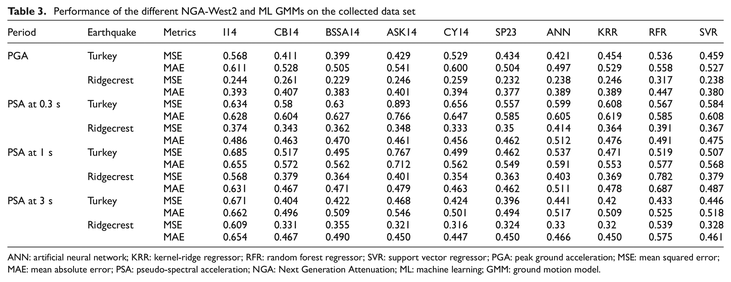
ANN: artificial neural network; KRR: kernel-ridge regressor; RFR: random forest regressor; SVR: support vector regressor; PGA: peak ground acceleration; MSE: mean squared error; MAE: mean absolute error; PSA: pseudo-spectral acceleration; NGA: Next Generation Attenuation; ML: machine learning; GMM: ground motion model.

Summary and conclusion

This study attempts to develop a new suite of global GMMs to predict different GMIMs for shallow crustal earthquakes in active regions having the key features of ground motions such as moment magnitude, R_rup, Z_TOR, and V_S₃₀ to include the source, path, depth, and site effects. In this regard, we use a subset of the NGA-West2 database, including 14,518 ground motion recordings out of 285 earthquakes. With growing interest in using ML techniques and increasing the size of the data set and number of recordings, we built four different data-driven nonparametric ML models to perform regression analysis. We used a repeated tenfold CV procedure to find the best hyperparameters for each estimator. The final ensemble model averages individual models’ outputs to compute the horizontal component of RotD50 PGA, 5%-damped PSA at different spectral periods, PGV, and PGD. Ensemble modeling aims to capture all benefits from individual models, increase accuracy, and improve predictions for future events. With no assumptions about the functional form, the developed ensemble GMMs can account for salient features of earthquake ground motions such as magnitude and distance scaling, saturation effect, magnitude-dependent hinge point, and linear and nonlinear site effects. A mixed-effects regression is used to partition the total residuals into between- and within-event components. Then, a smaller subset of the selected data is used to perform another mixed-effects regression to split the within-event variability into within-station and event-site–corrected residuals for site-specific applications. Finally, ensemble GMMs were compared and validated with the predicted PGA and PSA values from GMMs developed for the NGA-West2 database. Generally, there is good agreement between expected GMIMs from our GMMs using fewer explanatory variables with the NGA-West2 GMMs, including complex terms and results from simulations. The proposed GMMs generally have slightly lower standard deviations at longer periods and outperform the NGA-west2 GMMs in the mid-range period compared with observed ground motions from two recent large earthquakes. This new set of GMMs does not reject or supersede any other GMMs developed using the NGA-West2 data set, but it creates another predictive model that can help capture the uncertainty for seismic hazard analysis.

The ensemble GMMs for shallow crustal earthquakes in active regions are generally applicable for events with moment magnitudes ranging from 3 to 8, rupture distances up to 300 km, depth to the top of rupture less than 20 km, and V_S₃₀ between 150 and 1500 m/s. The proposed GMMs are global, and the user based on the region of interest may require performing some post-processing steps such as analysis of residuals and addition of regional path and site terms to account for systemic differences in those terms. It should be noted that the conventional regression method is still a better tool where limited data are available; however, the enriched NGA-West2 data set allows us to use the ML algorithms.

Data and resources

The Python computational platform and the scikit-learn package were used in our study to train all models. We used the PGA and response spectra of shallow crustal ground motion recordings and related metadata that were compiled and processed by the NGA-West2 project and provided to us by a flatfile publicly available at https://peer.berkeley.edu/research/data-sciences/databases.

The “Updated_NGA_West2_Flatfile_RotD50_d050_public_version.xlsx” file includes all the data. The “NGAW2_GMPE_Spreadsheets_v5.7_041415_ProtectedLocked.xlsm” file as well as the MATLAB codes provided by Jack Backer on GitHub (https://github.com/bakerjw/GMMs/tree/master/gmms) was used for comparison with other NGA-West2 GMMs.

The information for the 2019 M7.1 Ridgecrest and 2023 M7.8 Turkey earthquakes can be found at https://earthquake.usgs.gov/earthquakes/eventpage/ci38457511/executive and https://earthquake.usgs.gov/earthquakes/eventpage/us6000jllz/executive. The RotD50 GMIMs for the Ridgecrest earthquake are available on https://www.strongmotioncenter.org/specialstudies/rekoske_2019ridgecrest/. The showcase code and the saved models can be downloaded from the following GitHub repository. Since a pipeline framework has been used in Python, there is no need to process/normalize the input data for prediction and the saved models using pipeline take care of this step. The example in the showcase code is self-explanatory and can be accessed at https://github.com/farhadseda/ML-Based-GMMs-for-NGA-West2.

Supplemental Material

sj-docx-1-eqs-10.1177_87552930231191759 – Supplemental material for Machine learning–based ground motion models for shallow crustal earthquakes in active tectonic regions

Supplemental material, sj-docx-1-eqs-10.1177_87552930231191759 for Machine learning–based ground motion models for shallow crustal earthquakes in active tectonic regions by Farhad Sedaghati and Shahram Pezeshk in Earthquake Spectra

Footnotes

Acknowledgements

The authors thank Helen Crowley, Jeff Bayless, and two anonymous reviewers for their thoughtful comments and reviews that significantly improved this article.

Declaration of conflicting interests

The author(s) declared no potential conflicts of interest with respect to the research, authorship, and/or publication of this article.

Funding

The author(s) received no financial support for the research, authorship, and/or publication of this article.

ORCID iD

Shahram Pezeshk

Supplemental material

Supplemental material for this article is available online.

References

Abrahamson

Silva

Kamai

(2014) Summary of the ASK14 ground motion relation for active crustal regions. Earthquake Spectra 30: 1025–1055.

Ahumada

Altunkaynak

Ayoub

(2015) Fuzzy logic logic-based attenuation relationships of strong motion earthquake records. Expert Systems with Applications 42(3): 1287–1297.

Alavi

Gandomi

(2011) Prediction of principal ground motion parameters using a hybrid method coupling artificial neural networks and simulated annealing. Computers & structures 89(23/24): 2176–2194.

Ancheta

Darragh

Stewart

Seyhan

Silva

Chiou

BSJ

Wooddell

Graves

Kottke

Boore

Kishida

Donahue

(2014) NGA-West2 database. Earthquake Spectra 30: 989–1005.

Atik

Abrahamson

(2010) Nonlinear site response effects on the standard deviations of predicted ground motions. Bulletin of the Seismological Society of America 100: 1288–1292.

Atik

Youngs

(2014) Epistemic uncertainty for NGA-West2 models. Earthquake Spectra 30: 1301–1318.

Atkinson

(2008) Alternative ground-motion prediction equations for eastern North America from a referenced empirical approach: Implications for epistemic uncertainty. Bulletin of the Seismological Society of America 98: 1304–1318.

Atkinson

(2010) Ground-motion prediction equations for Hawaii from a referenced empirical approach. Bulletin of the Seismological Society of America 100(2): 751–761.

Bindi

(2017) The predictive power of ground-motion prediction equations. Bulletin of the Seismological Society of America 107: 1005–1011.

10.

Boore

(2003) Simulation of ground motion using the stochastic method. Pure and Applied Geophysics 160: 635–676.

11.

Boore

(2009) Comparing stochastic point-source and finite-source ground-motion simulations: SMSIM and EXSIM. Bulletin of the Seismological Society of America 99: 3202–3216.

12.

Boore

(2010) Orientation-independent, nongeometric-mean measures of seismic intensity from two horizontal components of motion. Bulletin of the Seismological Society of America 100: 1830–1835.

13.

Boore

Stewart

Seyhan

Atkinson

(2014) NGA-West2 equations for predicting PGA, PGV, and 5% damped PSA for shallow crustal earthquakes. Earthquake Spectra 30: 1057–1085.

14.

Bozorgnia

Abrahamson

Atik

Ancheta

Atkinson

Baker

Baltay

Boore

Campbell

Chiou

BS-J

Darragh

Day

Donahue

Graves

Gregor

Hanks

Idriss

Kamai

Kishida

Kottke

Mahin

Rezaeian

Rowshandel

Seyhan

Shahi

Shantz

Silva

Spudich

Stewart

Watson-Lamprey

Wooddell

Youngs

(2014) NGA-West2 research project. Earthquake Spectra 30: 973–987.

15.

Brownlee

(2016a) Machine learning algorithms from scratch with Python. Machine Learning Mastery. Available at: https://machinelearningmastery.com/machine-learning-algorithms-from-scratch/ (accessed 30 June 2023).

16.

Brownlee

(2016b) Overfitting and underfitting with machine learning algorithms. Machine Learning Mastery 21: 575.

17.

Brownlee

(2018) A Gentle Introduction to k-Fold Cross-Validation. Available at: https://machinelearningmastery.com/overfitting-and-underfitting-with-machine-learning-algorithms/ (accessed 30 June 2023).

18.

Brownlee

(2020) Repeated k-Fold Cross-Validation for model evaluation in Python. Machine Learning Mastery. Available at: https://machinelearningmastery.com/repeated-k-fold-cross-validation-with-python/ (accessed 30 June 2023).

19.

Campbell

(2003) Prediction of strong-ground motion using the hybrid empirical method and its use in the development of ground-motion (attenuation) relations in eastern North America. Bulletin of the Seismological Society of America 93: 1012–1033.

20.

Campbell

Bozorgnia

(2014) NGA-West2 ground motion model for the average horizontal components of PGA, PGV, and 5% Damped Linear Acceleration Response Spectra, earthquake. Spectra 30: 1087–1115.

21.

Chiou

BSJ

Youngs

(2014) Update of the Chiou and Youngs NGA model for the average horizontal component of peak ground motion and response spectra. Earthquake Spectra 30: 1117–1153.

22.

Collins

Graves

Somerville

(2006) Revised analysis of 1-D Rock Simulations for the NGA-E Project. Final report prepared for the Pacific Earthquake Engineering Research Center, University of California, Berkeley, CA, April.

23.

Derras

Bard

Cotton

(2014) Towards fully data driven ground-motion prediction models for Europe. Bulletin of the Seismological Society of America 12(1): 495–516.

24.

Derras

Bard

Cotton

Bekkouche

(2012) Adapting the neural network approach to PGA prediction: An example based on the KiK-net data. Bulletin of the Seismological Society of America 102: 1446–1461.

25.

Dhanya

Raghukanth

STG

(2018) Ground motion prediction model using artificial neural network. Pure and Applied Geophysics 175: 1035–1064.

26.

Donahue

Abrahamson

(2014) Simulation-based hanging wall effects. Earthquake Spectra 30: 1269–1284.

27.

Douglas

(2003) Earthquake ground motion estimation using strong-motion records: A review of equations for the estimation of peak ground acceleration and response spectral ordinates. Earth-Science Reviews 61: 43–104.

28.

Douglas

(2011) Ground Motion Prediction Equations 1964–2010. PEER Report No. 2011/ 102, Pacific Earthquake Engineering Research Center, University of California, Berkeley, CA, April.

29.

García

Romo

Mayoral

(2007) Estimation of peak ground accelerations for Mexican subduction zone earthquakes using neural networks. Geofísica Internacional 46: 51–63.

30.

Gök

Kaftan

(2022) Prediction of peak ground acceleration by artificial neural network and adaptive neuro-fuzzy inference system. Annales Geophysicae 65(1): SE106–SE106.

31.

Gregor

Abrahamson

Atkinson

, et al (2014) Comparison of NGA-West2 GMPEs. Earthquake Spectra 30(3): 1179–1197.

32.

Güllü

(2012) Prediction of peak ground acceleration by genetic expression programming and regression: A comparison using likelihood-based measure. Engineering Geology 141: 92–113.

33.

Zhang

(2022) Support vector machine method for developing ground motion models for earthquakes in Western part of China. Journal of Earthquake Engineering 26: 5679–5694.

34.

Idriss

(2014) An NGA-West2 empirical model for estimating the horizontal spectral values generated by shallow crustal earthquakes. Earthquake Spectra 30: 1155–1177.

35.

Kale

Akkar

(2013) A new procedure for selecting and ranking ground-motion prediction equations (GMPEs): The Euclidean distance-based ranking (EDR) method. Bulletin of the Seismological Society of America 103: 1069–1084.

36.

Kamai

Abrahamson

Silva

(2014) Nonlinear horizontal site amplification for constraining the NGA-West2 GMPEs. Earthquake Spectra 30: 1223–1240.

37.

Khosravikia

Clayton

(2021) Machine learning in ground motion prediction. Computers & Geosciences 148: 104700.

38.

Khosravikia

Clayton

Nagy

(2019) Artificial neural network-based framework for developing ground-motion models for natural and induced earthquakes in Oklahoma, Kansas, and Texas. Seismological Research Letters 90: 604–613.

39.

Kong

Trugman

Ross

Bianco

Meade

Gerstoft

(2019) Machine learning in Seismology: Turning data into insights. Seismological Research Letters 90(1): 3–14.

40.

Kotha

Bindi

Cotton

(2016) Partially non-ergodic region specific GMPE for Europe and Middle-East. Bulletin of Earthquake Engineering 14: 1245–1263.

41.

Kotha

Weatherill

Bindi

Cotton

(2020) A regionally-adaptable ground-motion model for shallow crustal earthquakes in Europe. Bulletin of Earthquake Engineering 18(9): 4091–4125.

42.

Kubo

Kunugi

Suzuki

Aoi

(2020) Hybrid predictor for ground-motion intensity with machine learning and conventional ground motion prediction equation. Scientific Reports 10(1): 1–12.

43.

Kuhn

Johnson

(2013) Applied Predictive Modeling. New York: Springer.

44.

Mak

Clements

Schorlemmer

(2017) Empirical evaluation of hierarchical ground-motion models: Score uncertainty and model weighting. Bulletin of the Seismological Society of America 107(2): 949–965.

45.

Parker

Stewart

Boore

Atkinson

Hassani

(2022) NGA-subduction global ground motion models with regional adjustment factors. Earthquake Spectra 38: 456–493.

46.

Petersen

Moschetti

Powers

Mueller

Haller

Frankel

Zeng

Rezaeian

Harmsen

Boyd

Field

(2015) The 2014 United States national seismic hazard model. Earthquake Spectra 31: S1–S30.

47.

Pezeshk

Zandieh

Campbell

Tavakoli

(2018) Ground-motion prediction equations for Central and Eastern North America using the hybrid empirical method and NGA-West2 Empirical Ground-Motion Models. Bulletin of the Seismological Society of America 108(4): 2278–2304.

48.

Raschka

(2018) MLxtend: Providing machine learning and data science utilities and extensions to Python’s scientific computing stack. Journal of Open Source Software 3(24): 638.

49.

Rekoske

Thompson

Moschetti

Hearne

Aagaard

Parker

(2019) Ground Motions from the 2019 Ridgecrest, California, Earthquake Sequence. Center for Engineering Strong Motion Data (CESMD). DOI: 10.5066/P9REBW60.

50.

Rekoske

Thompson

Moschetti

Hearne

Aagaard

Parker

(2020) The 2019 Ridgecrest, California, earthquake sequence ground motions: Processed records and derived intensity metrics. Seismological Research Letters 91(4): 2010–2023.

51.

Rodriguez-Marek

Rathje

Bommer

Scherbaum

Stafford

(2014) Application of single-station sigma and site-response characterization in a probabilistic seismic-hazard analysis for a new nuclear site. Bulletin of the Seismological Society of America 104: 1601–1619.

52.

Scherbaum

Delavaud

Riggelsen

(2009) Model selection in seismic hazard analysis: An information-theoretic perspective. Bulletin of the Seismological Society of America 99(6): 3234–3247.

53.

Schmedes

Archuleta

(2008) Near-source ground motion along strike-slip faults: Insights into magnitude saturation of PGV and PGA. Bulletin of the Seismological Society of America 98: 2278–2290.

54.

Schwarz

(1978) Estimating the dimension of a model. Annals of Statistics 6(2): 461–64.

55.

Sedaghati

Pezeshk

(2016) Comparative study on parameter estimation methods for attenuation relationships. Journal of Geophysics and Engineering 13: 912–927.

56.

Sedaghati

Pezeshk

(2017) Partially nonergodic empirical ground motion models for predicting horizontal and vertical PGV, PGA, and 5% damped linear acceleration response spectra using data from the Iranian plateau. Bulletin of the Seismological Society of America 107: 934–948.

57.

Sedaghati

Ansari

Farjooid

(2009) Developing attenuation relations by use of fuzzy logic and comparison to current relations for the Iranian Plateau. In: 5th National Civil Engineering Conference (in Persian). Mashhad, Iran.

58.

Sreenath

Raghukanth

STG

(2023) Stochastic ground motion models to NGA-West2 and NGA-Sub databases using Bayesian neural network. Earthquake Engineering & Structural Dynamics 52: 248–267.

59.

Sreenath

Podili

Raghukanth

STG

(2023) A hybrid non-parametric ground motion model for shallow crustal earthquakes in Europe. Earthquake Engineering & Structural Dynamics 52: 2303–2322.

60.

Stafford

(2014) Crossed and nested mixed-effects approaches for enhanced model development and removal of the ergodic assumption in empirical ground-motion models. Bulletin of the Seismological Society of America 104: 702–719.

61.

Stone

(1974) Cross-validation and multinomial prediction. Biometrika 61: 509–515.

62.

Tavakoli

Sedaghati

Pezeshk

(2018) An analytical effective point-source-based distance-conversion approach to mimic the effects of extended faults on seismic hazard assessment. Bulletin of the Seismological Society of America 108: 742–760.

63.

Tezcan

Cheng

(2012) Support vector regression for estimating earthquake response spectra. Bulletin of the Seismological Society of America 10: 1205–1219.

64.

Vemula

Sreejaya

Raghukanth

STG

(2023) Neural network-based subduction ground motion model and its application to New Zealand and the Andaman and Nicobar Islands. Journal of Earthquake Engineering 27: 2863–2886.

65.

Wooddell

Abrahamson

(2014) Classification of main shocks and aftershocks in the NGA-West2 database. Earthquake Spectra 30: 1257–1267.

Supplementary Material

Please find the following supplemental material available below.

For Open Access articles published under a Creative Commons License, all supplemental material carries the same license as the article it is associated with.

For non-Open Access articles published, all supplemental material carries a non-exclusive license, and permission requests for re-use of supplemental material or any part of supplemental material shall be sent directly to the copyright owner as specified in the copyright notice associated with the article.

0.00 MB

0.02 MB