Time-varying damping ratios and velocities in a high-rise during earthquakes and ambient vibrations from coda wave interferometry

Abstract

Coda wave interferometry is applied to data from Community Seismic Network MEMS accelerometers permanently installed on nearly every floor of a 52-story steel moment-and-brace frame building in downtown Los Angeles. Wavefield data from the 2019 M7.1 Ridgecrest, California earthquake sequence are used to obtain impulse response functions, and time-varying damping ratios and shear-wave velocities are computed from them. The coda waves are used because of their increased sensitivity to changes in the building’s properties, and the approach is generalized to show that a building’s nonlinear response can be monitored through time-varying measurements of representative pseudo-linear systems in the time domain. The building was not damaged, but temporary nonlinear behavior observed during the strong motions provides a unique opportunity to test this method’s ability to map time-varying properties. Reference damping parameters and velocities are obtained from a month-long period during which no significant seismic activity had occurred. Damping ratios measured over narrow frequency bands increase by up to a factor of 4 over short time durations spanning the main shock, as well as M > 4.5 aftershocks and a foreshock. The largest damping ratio increases occur for the highest frequencies, and the increase is attributed to friction associated with structural and non-structural surface discontinuities which experience relative motion and impact during shaking, resulting in energy loss. Shear-wave velocities in the building’s east–west and north–south directions are found by applying a waveform stretching method to the direct and coda waves. The broadband velocities are reduced by as much as 10% during building shaking, and their restoration to pre-earthquake levels is found to be a function of shaking amplitudes. Until recently, these techniques had been limited by temporal and spatial sparsity of measurements, but in this study, variations of the impulse response functions are resolved over time scales of tens of seconds and on a floor-by-floor spatial scale.

Keywords

Monitoring impulse response health monitoring seismology coda wave interferometry

Introduction

We introduce the application of coda wave interferometry (CWI) to very high-resolution high-rise data, both spatially and temporally, to extract time-varying properties, including damping ratios and shear-wave velocities. These are obtained from propagating impulse response functions (IRFs) due to building excitations during the 2019 M7.1 Ridgecrest California earthquake sequence. The CWI method employed here takes advantage of the delay in the later wave arrivals. Because of the use of both direct and later arrivals, this technique has greater sensitivity to slight changes in the medium (here, a building’s inelastic properties), particularly when the full waveform can be compared before and after repeated sources, such as anthropogenic noise sources and earthquakes. We show how a building’s nonlinear response can be continuously resolved and monitored over very short time segments (order of 20 s) in a quantitative, signal-processing approach that uses the IRF coda waves. Understanding the mechanics behind the analogous data signatures of building damage caused by shaking, for example, the increase in damping ratios and reduction in seismic velocities due to earthquake excitation could provide insights into designing structural health monitoring (SHM) and damage detection tools.

Interferometric techniques are based on cross-correlation or deconvolution of seismic wavefields at two different locations between which constructive interference produces coherent waves. Inside buildings, cross-correlated deconvolved wavefields represent wave propagation between any two floors. These techniques have been applied to earthquake data (Kohler et al., 2007; Nakata and Snieder, 2014; Nakata et al., 2013; Rahmani and Todorovska, 2021; Rahmani et al., 2015, 2017; Snieder and Safak, 2006; Todorovska and Trifunac, 2008a, 2008b) and ambient vibration data (Nakata and Snieder, 2014; Prieto et al., 2010; Sun et al., 2017) to extract the building characteristics associated with the IRFs, such as seismic velocity, broadband damping, and the time-lapse changes in these properties. After cross-correlation or deconvolution, the response of the building that has been extracted is independent from the ground motion, soil–structure interaction, and complex earthquake source signature. With interferometric techniques, we can modify the boundary conditions through our choice of receiver pairs to obtain a richer, information-filled set of propagating wave characteristics. We often assume that wave propagation in the building is one-dimensional for simplicity (Nakata et al., 2013; Snieder and Safak, 2006); this assumption holds well for intermediate- to high-rise buildings excited by earthquake motions at their base (Celebi et al., 2016) though it is not a necessary assumption (Ebrahimian and Todorovska, 2014, 2015). The extracted IRF waveforms represent the reverberation of waves between the two floors with amplitude and polarity that depends on the reflection boundary conditions. Time-domain IRFs are typically computed for waves propagating between the ground level and the top of the building, and are examined for damage signatures which could result in velocity reduction.

Seismic interferometric techniques applied to the arrays of seismometers deployed on the surface of the Earth have been successful at imaging seismic velocities within the solid Earth, from delineating oil reservoirs to identifying inelastic, non-isotropic seismic heterogeneity in the deep Earth. Measurements of the time-varying seismic velocity field (often reductions in wave speeds) in regions temporarily subjected to strong ground motions are a small but growing practice due to the wide availability of seismic records with the spatial and temporal resolution to resolve those changes (Brenguier et al., 2008a; Mordret et al., 2016; Nakata and Snieder, 2011; Peng and Ben-Zion, 2006; Rubinstein and Beroza, 2004a, 2004b; Sawazaki et al., 2006; Sheng et al., 2022).

The traditional derivation of the IRF arises from equations of motion for linear elastic systems. In SHM applications, the impulse response of the structure is useful because it can be measured as the displacement at any location that is produced in response to an input or “virtual source” forcing function at another location. Time-domain IRFs of mid-rise and high-rise structures provide information about system response that is complementary to frequency response functions and response spectra (e.g. Ebrahimian et al., 2018). IRFs provide information about pre-event and post-event (including for the nonlinear case) perturbations in reflection coefficients, dispersion effects, damping, travel times, and traveling wave velocities. In traditional IRF computations, it is usually implicitly or explicitly assumed that the IRF is computed with respect to a baseline response in which no large amplitude applied load has recently affected the system, altering its dynamic properties. Here, we use a month-long period of ambient vibration recordings during which no significant seismicity near the building had occurred, for the baseline response.

In this study, we also compute damping ratios from the IRFs for different frequency bands. Early studies on damping introduced the viscous damping coefficient with corresponding physical mechanisms as a mathematically convenient way to describe energy dissipation in structures (Hudson, 1965; Jacobsen, 1930, 1960; Soroka, 1949). The introduction of electronic structural vibration sensors deployed inside full-scale structures that included buildings and towers made it possible to measure damping from ambient vibrations (Abazarsa et al., 2013; Zhang and Cho, 2009), wind events (e.g. Jeary, 1992; Lagomarsino, 1993; Tamura and Suganuma, 1996), and earthquakes (Celebi et al., 2017; Ghahari et al., 2012; Goel and Chopra, 1997; Hart and Vasudevan, 1975; Satake et al., 2003). Specific to this study, Jeary (1992) introduced the idea of using the random decrement technique to measure the first-mode damping of two towers subjected to wind loading. Hart and Vasudevan (1975) measured damping from 12 high-rise buildings using data from the 1971 San Fernando, CA earthquake using a frequency-domain identification technique. McVerry (1979, 1980) found better matches for damping in the same buildings with a similar dataset by computing damping associated with the fundamental period for small-time series segments. Not long after, studies using a range of input excitations began showing that damping ratios depend on the vibration amplitude (Jeary and Ellis, 1984; McVerry, 1979, 1980; Satake et al., 2003; Tamura and Suganuma, 1996). Additional studies illustrated differences in damping resulting from differences in building type and foundation type (Bernal et al., 2015, 2012; McVerry, 1980; Miranda and Cruz, 2017; Reinoso and Miranda, 2005; Satake et al., 2003). Soil–structure interaction was found to play a role in the expected energy dissipation resulting in variations in damping ratio estimation (Bernal et al., 2015; Miranda and Cruz, 2017; Zhang and Cho, 2009). Miranda and Cruz (2017) found that damping ratios of higher modes increase approximately linearly with increasing frequency but do not correspond to a mass- or stiffness-proportional damping model. State-space identification techniques to estimate modal parameters including damping ratios are now common (Ghahari et al., 2012; Reinoso and Miranda, 2005), allowing for the estimation of non-classical damping (Ghahari et al., 2016).

A common theme in most prior damping studies is that they use frequency-domain methods or rely on the identification of modal parameters to measure the damping ratio. Our study is a complementary approach to measuring damping ratios over a broad range of frequencies entirely from time-domain IRFs. In addition, using data from a spatially dense array allows us to resolve damping over very small-time scales—on order of 20 s over the course of a single earthquake input. Our method does not depend on identifying modal parameters (e.g. frequencies and mode shapes) or assuming models (e.g. SDOF, Timoshenko beam) to find the associated damping ratios.

Compared with frequency-domain IRFs, the time-domain interferometric techniques including the coda waves have at least two clear advantages. The first is that the signals do not need to be decomposed into different structural resonant modes. Even though the first few modes for most intermediate- to high-rise buildings may be identifiable, the higher-frequency modes often necessary for the dynamic analysis and small-scale damage detection and location are usually not easily identified in the frequency domain with low uncertainty. The second advantage is that this cross-correlation method needs only very short time intervals for the averaging to extract high signal-to-noise IRFs (Ebrahimian and Todorovska, 2015; Todorovska and Trifunac, 2008a, 2008b). Therefore, the response changes can be extracted for even just one hazard event (e.g. earthquake or strong wind event). Quantifying these short time changes with CWI, as we show here, has the potential to aid in characterizing the nonlinear response of the system with better spatial resolution.

Data

The July 2019 Ridgecrest, California earthquake sequence occurred in southeastern California, a few kilometers northeast of the city of Ridgecrest (Ross et al., 2019). The mainshock consisted of an M7.1 earthquake on 6 July 2019, preceded 2 days earlier by an M6.4 foreshock. Light-to-moderate ground shaking from both the M6.4 and M7.1 Ridgecrest earthquakes was felt in the greater Los Angeles region, located about 200 km from the epicentral region (Figure 1a). High-rises experienced unusually strong long-period shaking in the east–west direction, as a result of excitation by complex trains of scattered shear waves, followed by surface waves propagating into the Los Angeles basin.

Figure 1.

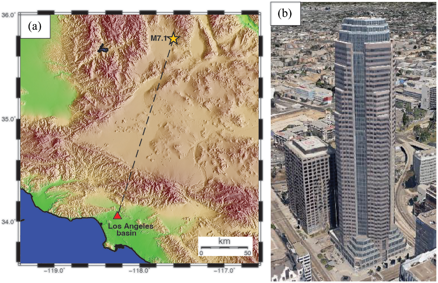
(a) Ridgecrest M7.1 earthquake location (yellow star) and downtown Los Angeles where the 52-story is located (red triangle) and (b) 52-story building in downtown Los Angeles (image from Google Earth).

The 2019 Ridgecrest earthquake sequence was recorded on hundreds of regional strong-motion network sensors in the Los Angeles basin. In particular, the community-hosted Community Seismic Network (CSN) captured variations in ground-level motion and upper floor shaking within mid-rise and high-rise buildings on triaxial accelerometers deployed on nearly every floor (Kohler et al., 2020). The CSN (Clayton et al., 2015, 2020) consists of inexpensive micro-electromechanical systems (MEMS) accelerometers that operate and record acceleration waveform data continuously at 50 sps within ± 2 g maximum amplitude levels. The sensors relay continuous 24/7/365 acceleration waveform data and shaking intensity parameters using the Amazon Web Services cloud environment. The network consists of about 1200 sensors located mainly in the Los Angeles basin, both at ground-level locations and in the upper floors of mid-rise and high-rise structures (Kohler et al., 2014, 2016, 2020) CSN has instrumented several mid-rise and high-rise structures, one of which is a 52-story (+ five subterranean garage levels) dual-steel moment-and-brace frame building located in downtown Los Angeles (Figure 1b). This building’s lateral system consists of a braced frame core surrounded by a steel moment frame. The floor plans contain various setbacks and notches along the building’s vertical profile. The structural system consists of three major components: an interior concentrically braced core, outrigger beams spanning the core to the building perimeter, and eight exterior outrigger columns. The beams support gravity loads, act as ductile moment-resisting beams between the core and exterior frame columns, and enhance the overturning resistance of the building by engaging the perimeter columns to the core columns (Taranath, 1997). The first five translational resonant frequencies of this building in the horizontal directions are approximately 0.2, 0.6, 1.2, 1.7, and 2.2 Hz (Celebi et al., 2016; Kohler et al., 2016). This building recorded the Ridgecrest earthquakes on triaxial CSN sensors deployed on most floors of the building (see Figure 3 in the work by Kohler et al., 2020).

CWI

This technique takes advantage of the sensitivity of coda waves to small changes in the medium by comparing the waveforms before and after a perturbation. Coda waves, in this setting, are the waves that have been scattered multiple times, for example, from the boundaries or different floors of the building. The idea has been used for estimating velocity changes in fault zones (Poupinet et al., 1984), volcanoes (Grêt et al., 2005), and in ultrasonic experiments (Planès and Larose, 2013). It has also been applied to monitoring engineering structures (Serra et al., 2017; Stähler et al., 2011; Wang et al., 2022), detecting damage in concrete samples (Fröjd and Ulriksen, 2017; Planès and Larose, 2013), and even detecting minute changes associated with fluid migration in rocks (Desmond and Valenza, 2019). However, it has not been used in SHM of buildings, with only a couple of exceptions for velocity variations (Jaimes et al., 2022; Mordret et al., 2017), but not for damping.

For CWI to be useful, a repeating source is required. This could be repeating or doublet earthquakes (Grêt et al., 2005; Poupinet et al., 1984), a repeating active source (e.g. hammer blows as in the work by Stähler et al., 2011), or waveforms obtained by seismic interferometry (Brenguier et al., 2008a, 2008b; Sens-Schönfelder and Wegler, 2006). In our case, the IRFs obtained by deconvolution represent such a repeating experiment (Jaimes et al., 2022) in which we use a longer train of IRF waveforms that include coda waves.

CWI explained

Assume an unperturbed wavefield u(t) can be written as a path summation (Snieder, 2006) over all possible paths

u (t) = \sum_{P} A_{P} S_{P} (t - t_{P}) .

(1)

The path P is defined as the entire path that a particular wave packet has traveled, t_P is the travel time along the path, A_P is its amplitude, and S(t) is the source wavelet. The travel time for path P is

t_{P} = \int_{P} \frac{1}{v} ds

(2)

where the integration is along the path P. Figure 2 shows an example of how the wavefield u(t) can be constructed as a summation of different paths and how different paths (e.g. throughout a building) can have similar travel times.

Figure 2.

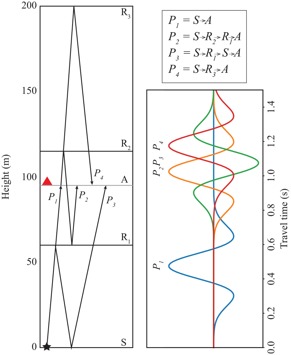
Construction of wavefield u(t) as a summation of four different paths inside a building. Paths always begin at the source S at the bottom of the building and are reflected from some combination of S, R₁, R₂, and R₃ floors. Paths are described in the top legend. The receiver is located at floor A (95 m height), the source has a Ricker wavelet, and the amplitude A_P is assumed to be unity for all paths. Note how paths P₂, P₃, and P₄ all arrive over a time span of below 0.2 s. The wavefield u(t) is the summation of the individual path wavefields.

Now, assume a perturbed wavefield

u_{per} (t) = \sum_{P} A_{P} S_{P} (t - t_{P} - τ_{P})

(3)

whose travel time is due to a velocity variation given by

t_{P} + τ_{P} = \int_{P} \frac{1}{v + δ v} ds = \int_{P} (\frac{1}{v} - \frac{δ v}{v^{2}}) ds .

(4)

We can solve for the travel-time perturbation

τ_{P} = - \int_{P} \frac{1}{v} \frac{δ v}{v} ds = - (\frac{δ v}{v}) \int_{P} \frac{1}{v} ds

(5)

where we have assumed that the relative velocity perturbation is constant, leading to

τ_{P} = - (\frac{δ v}{v}) t .

(6)

Note that we have assumed the velocity perturbation (dv/v) is constant, but the velocity v can change along the path. We have also replaced t_P by t, the average travel time over a window [t_P− T, t_P + T].

According to the previous expression, the travel-time perturbation depends on the travel time of the wave packet only and is independent of the path. That is, two paths that have similar travel times, even if very different trajectories, will have a similar travel-time perturbation. Thus, the mean travel-time perturbation can be estimated from the average of all trajectories or paths that arrive in the time window around t.

Figure 3 shows a comparison of two wavefields (with a more complete set of paths compared to Figure 2) where the perturbed wavefield (red trace) has a dv/v = −5% velocity perturbation. Note how the waveforms are similar, but the waves are increasingly out-of-phase as time becomes larger. We take three short windows at different times and, for each, find the travel-time perturbation τ between the two traces, shown in the bottom panel. Note that, as predicted before, the travel-time perturbation is larger as t grows, and the slope of τ/t is proportional to the velocity perturbation.

Figure 3.

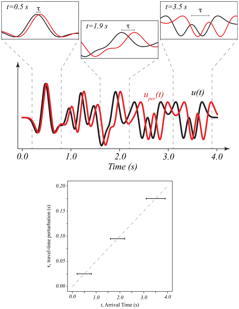
A comparison of wavefields before and after an applied velocity perturbation dv/v = −5% using the summation method in Equation 1. Selected windows are chosen to show how the travel-time perturbation can be estimated by looking at the phase delay of the two traces. Travel-time delay becomes larger as t increases. Bottom panel shows the estimated travel-time perturbation τ as a function of the average travel time at each selected window.

CWI velocity variations

We illustrate how focusing on different parts of the IRF wavefield, which reflect different combinations of wave paths, provides additional information. We define <τ> as the mean travel-time perturbation of all the wave paths over a short time window (t − T, t + T) and use this as a function of the travel time t, to estimate the velocity perturbation between two traces: a reference trace u(t) and a perturbed trace u_per(t). Snieder et al. (2002) and Snieder (2006) showed that the maximum of the cross-correlation between the two traces over the short time window provides the estimate of the velocity perturbation. We can see this in Figure 3, where the small windows show that the two traces are identical but time-shifted by τ, and the cross-correlation provides an estimate of that time shift. This can be done over several different small-time windows at different average travel times t (for example, Brenguier et al., 2008a; Snieder et al., 2002). The linear regression of time delay versus time in the coda (as in the bottom panel of Figure 3) is used to find the velocity perturbation.

Another approach, known as the stretching correlation method (Sens-Schönfelder and Wegler, 2006), estimates the relative delay time <τ> from the proportion by which the time axis t has to be compressed or dilated to obtain the highest correlation between the two traces. As pointed out by Sens-Schonfelder and Wegler (2006), the advantage of this approach is that dt/t does not need to be small, allowing for a stable estimate even when the velocity variations are of the order of 10% or more (see for example Figure 3, where the late window at t = 3.5 s only has 50% overlapping waveforms between the two traces).

Method and results

Estimating IRFs

In preparation for implementing CWI, we calculate the IRFs between pairs of sensors at different floors by computing the cross-correlation and normalizing by the power spectrum of the reference station using a multitaper algorithm (Prieto, 2022). This is equivalent to estimating the impulse response via deconvolution (Celebi et al., 2016; Jaimes et al., 2022; Prieto et al., 2010; Snieder and Safak, 2006), whereby the cross-spectrum of the two signals (the complex spectrum of one signal is multiplied by the complex conjugate of the complex spectrum of the second signal) is divided by the power spectrum of the reference signal. The resulting frequency-domain response is then inverse-Fourier-transformed and plotted as the IRF. In this study, we use both the direct and coda waves in a full-waveform analysis of shear-wave arrivals resulting from the deconvolutions. Note that the shear waves for this building are likely dispersive, but we focus on broadband shear-wave velocities.

The IRFs are obtained for time periods spanning the Ridgecrest mainshock on 6 July 2019, and a month of ambient vibrations recorded during a seismically quiet period in November 2021 when the largest number of sensors in the building was operating. In this study, we focus on deconvolving the acceleration waveforms recorded on every level of the 52-story building with respect to the waveforms at the ground level (Figure 4) and the top levels (Supplemental Figure A1). Because there is no sensor deployed on the first floor, the second floor is used as the reference location (“virtual source”) for the ground level, and the sensor at the 50th floor (the topmost sensor) is used as the reference station for the top level.

Figure 4.

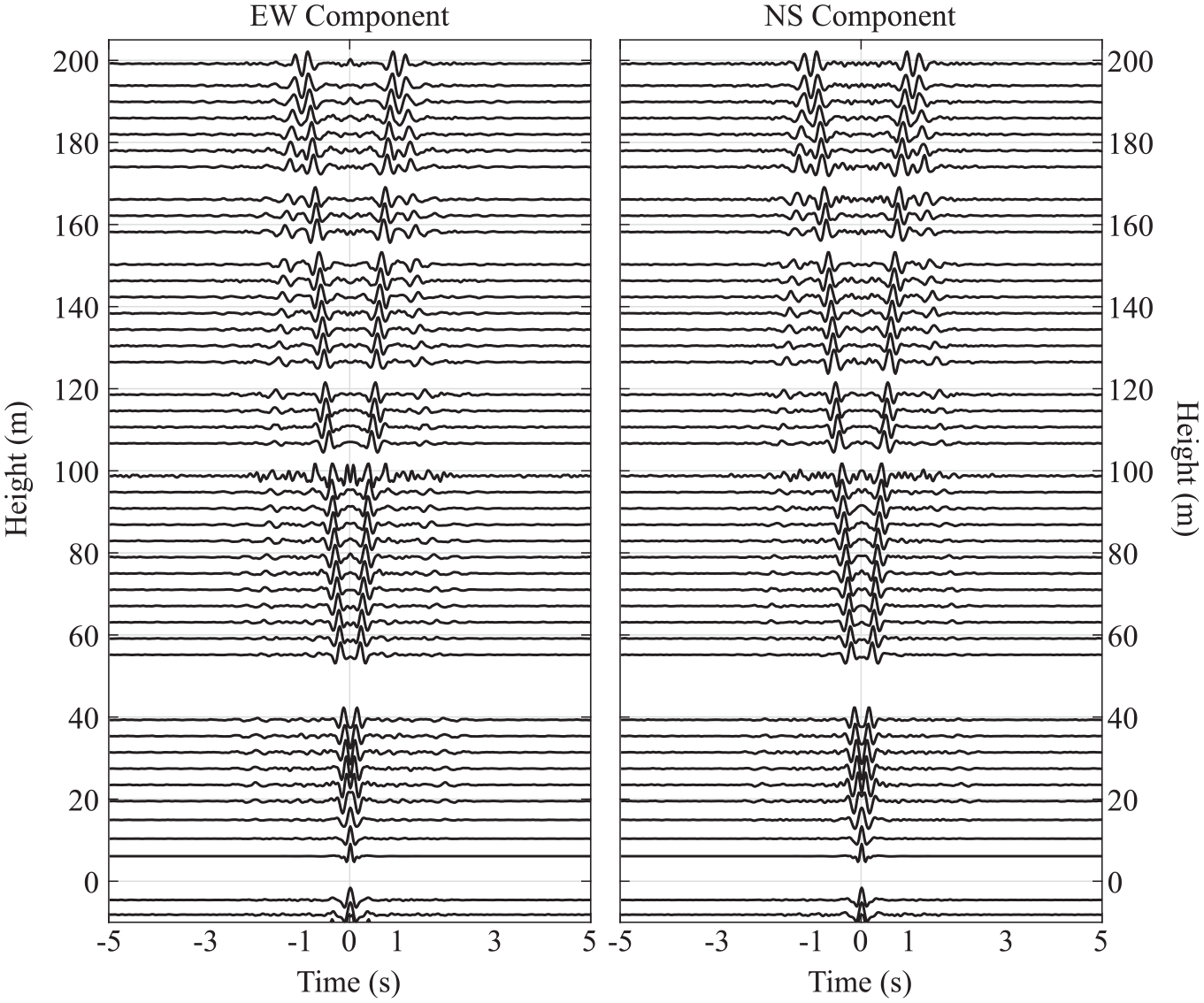
IRFs from the 52-story building for the two horizontal components (building-EW and building-NS) with respect to the sensor at Floor 2 computed from 30 min of earthquake data around the 2019 M7.1 Ridgecrest earthquake. Traces are filtered between 0.5 and 10 Hz.

During the periods when the building is still dynamically responding to the M7.1 Ridgecrest earthquake loading, or is in measurable free vibration from earthquake excitation, the waveforms are divided into 20-s-long segments. The 20-s windows are shifted at 10-s intervals (i.e. 50% overlap with the previous window), and the IRFs are estimated for each of these windows. No stacking is performed on any waveforms before or after cross-correlation for the 20-s periods. To obtain the pre-event baseline response, similar processing is applied to ambient vibration data. For this, we used 30 days of continuous data recorded from 1 to 30 November 2021 because this was a period of no significant seismicity and when a maximum number of sensors were recording data (i.e. minimum number of faulty stations). However, because the accelerations are much lower in amplitude, stacking is applied to 1-h-long files to obtain 30-day IRFs. As with the earthquake data, these represent shear waves in the building that are the IRFs between the reference floor and every other instrumented floor in the building.

Figure 5 shows a comparison of 30-day IRFs of ambient vibration data and IRFs obtained from a single 20-s window during strong shaking due to the Ridgecrest mainshock. These IRFs show that during earthquake shaking for the 20-s periods, clear IRFs emerge from the procedure. Figure 5 also shows that although both IRFs look alike, there is a clear phase shift between the traveling waves of the ambient vibration and strong shaking windows, suggesting a change in the wave speed within the building.

Figure 5.

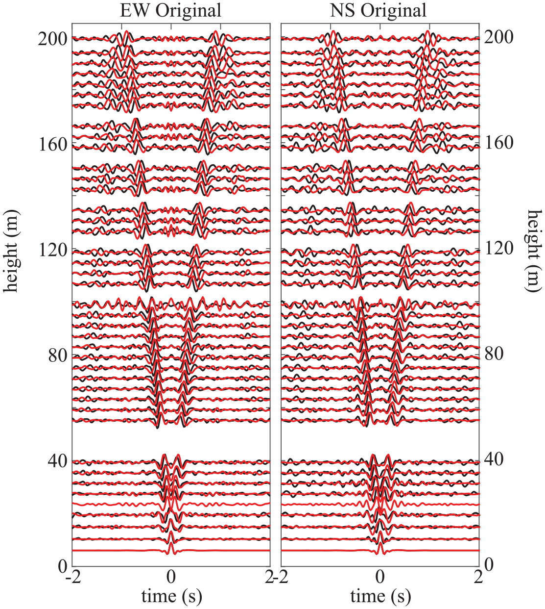
IRFs with respect to sensor at Floor 2 computed from ambient vibration data (black traces) and using 20-s window during strong shaking during the 2019 M7.1 Ridgecrest earthquake (red traces) for the building-EW (Left panel) and building-NS (Right panel) horizontal components. Traces are filtered between 0.5 and 10 Hz.

Estimating velocity variations with CWI

In this approach, we compare every set of 20-s IRFs with the reference 30-day IRFs obtained from ambient vibration data where no significant shaking is observed. As shown in Figure 5, a delayed arrival of the upgoing wave is clear for all traces, but it is also evident that later arrivals (e.g. downgoing waves reflected from the top of the building) are also delayed for the IRFs during strong shaking.

By estimating the time delays of the phases of the reference IRFs (from ambient vibrations) with respect to the IRFs during the M7.1 Ridgecrest earthquake, we obtain an estimate of the velocity perturbation (dv) inside the building. The advantage of such a method is that our estimate is based not only on the arrival times of the direct upgoing wave but also draws information from reflected waves within the IRFs, an ideal case for CWI.

To estimate the time delays for velocity variations, we use the stretching technique (Hadziioannou et al., 2009; Sens-Schönfelder and Wegler, 2006) whereby we stretch the time axis (±α%) of one waveform (e.g. the 20-s IRF) and compare the resulting traces with the unperturbed reference traces (the reference IRF). The optimal velocity perturbation α is obtained when the cross-correlation coefficient of all traces is maximum. Figure 6 shows the same IRF traces as in Figure 5 but the reference IRFs have been stretched by 8% and 10% in the EW and NS components. Note how, after the velocity perturbation correction, the two traces align along the entire waveform, including the upgoing and the downgoing wave. The correlation coefficient of the 39 traces before velocity correction is CC = 0.2; after velocity correction, it is increased to CC = 0.8.

Figure 6.

Velocity-corrected IRFs with respect to sensor at Floor 2 computed from ambient vibration data (black traces) and using 20-s window during strong shaking during the 2019 M7.1 Ridgecrest earthquake (black traces) for the building-EW (left panel) and NS horizontal components (right panel).Traces are filtered between 0.5 and 10 Hz.

We apply this method in an automated procedure to every 20-s window in the minutes before, during, and after the M7.1 Ridgecrest earthquake. Figure 7 shows the resulting velocity variations estimated using the CWI method. During the M7.1 strong motions, the velocity perturbation reaches a maximum reduction of about 10% that slowly recovers as the shaking amplitude decreases. An M4.9 earthquake occurring 3 min before the M7.1 is observed and generates a short-lived velocity reduction of around 5% that quickly recovers. The dashed vertical lines in Figure 7 show the origin times of M > 4.5 earthquakes (1 foreshock, the mainshock, and 11 aftershocks). For all these earthquakes (all of which occurred in approximately the same source region), the travel time for the first seismic arrivals at the building location is ∼30 s, and for shear waves it is ∼45 s.

Figure 7.

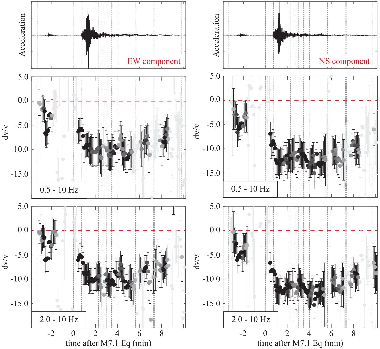
Estimated velocity variations (dv/v) for the building-EW (left-hand side) and building-NS (right-hand side) components using CWI applied to times before, during, and after the 2019 M7.1 Ridgecrest earthquake. Dashed vertical lines show origin times of M > 4.5 earthquakes (1 foreshock, mainshock, and 11 aftershocks). Top panels show waveforms recorded on 50th floor for reference. Lower panels show velocity variations at different frequency bands. Light gray circles and error bars represent IRFs with low correlation coefficients and thus have large uncertainties.

In Figure 7, we show estimated dv/v for the 20-s windows, with grayscale indicating the level of certainty where optimal correlation coefficients CC > 0.5 are shown in black. For the times when very low-amplitude signals are present, the computed 20-s IRFs are noisy and thus have a low correlation coefficient with respect to the reference IRF, irrespective of the velocity perturbation. We cannot use such windows to estimate the velocity perturbations because the uncertainties are much higher (it is impossible to define the phase delay of two uncorrelated traces).

In a separate test of consistency with modal observations, high-resolution spectrogram analysis indicates temporary drops in eigenfrequencies during the M7.1 Ridgecrest mainshock that are consistent with the IRF velocity observations discussed here. The spectrogram calculations are performed on the same building-EW accelerations in time windows that are 40 s long, and then shifted forward in time by 20 s (i.e. 50% overlap). The spectrograms show a 10% reduction in the first east–west translational mode (∼0.2 Hz), 8% reduction in the second translational mode (∼0.6 Hz), and 15% reduction in the third east–west translational mode (∼1.2 Hz) (Supplemental Figure A2a). In the building-NS direction, the reductions are 10% for the first north–south translational mode (∼0.2 Hz), 7% in the second north–south translational mode (∼0.6 Hz), and 12% in the third mode (∼1.2 Hz) (Figure A2b). The spectrograms also show how the eigenfrequency changes can be tracked in near real time relative to the types of seismic waves (and their associated frequency bands) that are exciting the building. As with the IRF properties, if the permanent damage events had occurred, the eigenfrequencies would be expected to register a permanent change (e.g. Clinton et al., 2006), without reverting to the pre-event levels.

Estimating damping variations

The damping ratios for narrow bands that correspond to modes can be computed by measuring the slope of the envelope of the IRFs, bandpass filtered within the half-power bandwidth (Mordret et al., 2017; Prieto et al., 2010; Snieder and Safak, 2006). Nakata and Snieder (2014) suggested that with ambient vibration deconvolution interferometry, when noise sources are inside the building, the damping ratio measured by the amplitude decay of the deconvolution function is a combination of the intrinsic damping of the building and the radiation loss in the solid Earth at the base of the building. The advantages are that damping ratios can be computed directly from the earthquake and ambient vibration data, without having to assume a model (e.g. shear beam: Rahmani et al., 2015, 2017, 2021) or approximation of the system (e.g. SDOF: Kashima, 2017; Kashima et al., 2014).

In this study, we compute both broadband and narrowband damping ratios (ξ) by filtering the EW and NS IRFs in several bands between 0.5 and 6.0 Hz and compare the amplitude decay of the 20-s IRF during strong shaking. We use IRFs with respect to the bottom level (Floor 2) (Figure 4), but we also compute the IRFs relative to the top level as an independent sanity check (Supplemental Figures A3–A4). Results with the top level are similar, and we therefore only present the bottom-level results here (see comparison in Figure A5). Before filtering, this analysis mixes information of multiple modes because the IRFs contain the response of a large range of frequencies. The narrow bands presented here include 0.5–1.0 Hz (which spans the second set of translational resonant frequencies in the horizontal directions), 0.8–1.3 Hz (spanning the third set of frequencies), 2–4 Hz (spanning the fifth set of frequencies), and 3–6 Hz which is above the fifth set of frequencies.

We estimate the damping factor by looking at the amplitude decay of the envelope of the IRFs with respect to the bottom level. In this case, we fit the logarithm of the amplitude of the IRFs at each floor with a linear function that is proportional to 2πftξ, where t is the travel time and ξ is the critical damping factor and we use f as the midpoint of the filtering band. We fit the linear decay starting at the predicted arrival time of the upgoing wave. Supplemental Figure A6 shows an example fit of the IRFs amplitude around the fundamental mode (0.18 Hz) at different heights using a 100-s-long window. Our method is thus also capable of estimating damping for the fundamental mode, but as our interest is in estimating temporal variations over short time windows, we focus on higher frequencies.

Similarly, we use the ambient vibration IRFs as a reference and compute the damping factor relative to the reference IRF envelope for the higher frequencies. This approach provides a more stable estimate of damping factor because the reference IRF has a similar envelope shape compared to the 20-s envelope; thus, the relative slope estimate is better constrained. Figure 8 shows 5 s of example IRF envelopes at three times during the strong shaking of the M7.1 Ridgecrest earthquake, where the amplitude decay is steeper for the IRFs associated with the strongest shaking (black circles, 1 min after origin time) and thus has a larger damping ratio. Supplemental Figure A7 shows examples of the misfit as a function of damping parameter for the three times in Figure 8, suggesting that the method can distinguish the damping variations presented here. The choice of the window length over which we perform our linear fit has a small, but non-negligible, effect on the damping estimate. When using too short of a window, the amplitude decay is negligible and the fit is not meaningful because there are too few datapoints to constrain it; using too long of a window incorporates a lot of background noise in the IRFs, leading to a flat amplitude decay, thus biasing the estimate toward background noise values. We tested different window lengths and settled on 5 s for all IRF envelopes.

Figure 8.

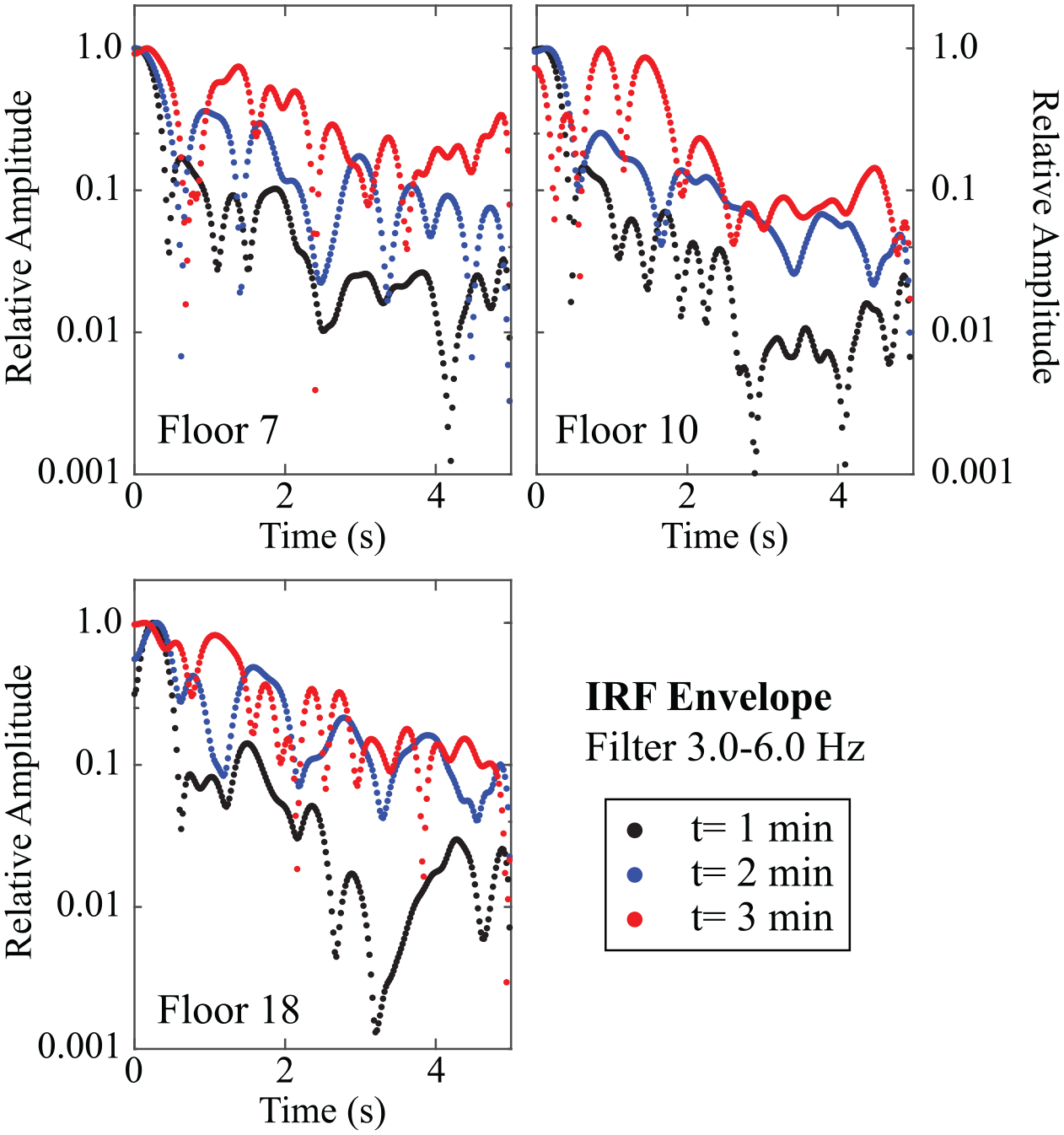
Log envelope amplitudes for IRFs with respect to the bottom floor for 3–6 Hz frequency range, for three floors: 7th, 10th, and 18th. Other floors look similar. Black circles: 20-s IRF corresponding to 1 min after Ridgecrest origin time. Blue circles: 20-s IRF corresponding to 2 min after Ridgecrest origin time. Red circles: 20-s IRF corresponding to 3 min after Ridgecrest origin time.

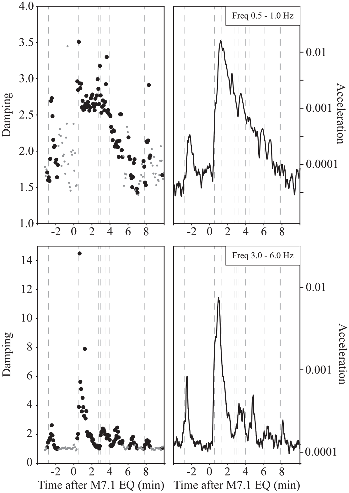
Figure 9 shows the estimated damping factors using the method presented here. Note the strong variations in damping just after the mainshock (time = 0.0 min) and even after a small foreshock (time approximately −3.5 min). The strong variation during the mainshock consists of a significant damping increase (more attenuation) that slowly recovers. Even after the initial damping increases, the recovery is not monotonic, but rather shows variations. In Figure 9, we mark the origin times of a foreshock, the mainshock, and M4 > 5 aftershock of the M7.1 earthquake, and we observe a clear time correlation between increases in the damping ratios and the arrival times of earthquake energy at the building location. As mentioned earlier, for all these earthquakes (all of which occurred in approximately the same source region), the travel time for the first seismic arrivals at the building location is ∼30 s and for shear waves, it is ∼45 s. This explains the delay time between each vertical line (origin time) and the onset of damping increase in these plots.

Figure 9.

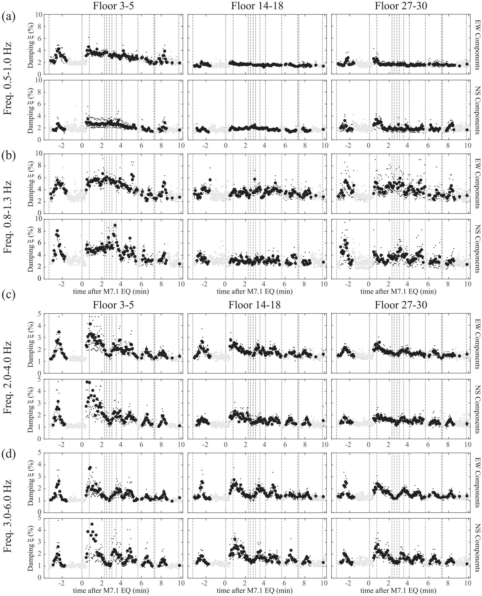
Comparison of damping estimates for building-EW (top rows in each panel) and building-NS components (bottom row in each panel) at different frequency bands for times before, during, and after the 2019 M7.1 Ridgecrest earthquake. (a) Frequencies between 0.5 - 1 Hz (b) 0.8 - 1.3 Hz (c) 2 - 4 Hz, and (d) 3 - 6 Hz. Vertical dashed lines mark the origin times of M > 4.5 earthquakes (1 foreshock, the mainshock, and 11 aftershocks). Smaller dots represent estimates at individual floors, while larger filled circles are averages over the floors for each column, each corresponding to a 20-s IRF window. Gray symbols correspond to noisy IRFs (see Figure 7).

The highest frequencies produce the most pronounced increases, with damping ratio increasing by up to a factor of 4 (∼1% to ∼4%) during the mainshock motions (Figure 9b to d), and increasingly small for lower frequencies (Figure 9a). The damping ratio increase lasts about 30–120 s, then reduces for a short duration before the M > 4.5 aftershock energy arrives at the building. In the context of the horizontal modes of this building, Figure 9a spans the second set of frequencies (0.5–1.1 Hz), Figure 9b spans the third set of translational modal frequencies (0.8–1.3 Hz), Figure 9c spans the fifth set of translational frequencies (2–4 Hz), and Figure 9d spans frequencies above the first five translational modal frequencies (3–6 Hz). This suggests that the high-frequency shaking associated with the aftershocks leads to temporary increases in the damping factor that are within the slow recovery of the initial damping increase due to the mainshock. The damping variations at low frequencies (Figure 9a) do not show these kinds of variations, while the higher-frequency damping factors are more or less aligned with the arrival of seismic energy from the aftershocks (Figure 9c and d).

To understand why the damping ratio changes over such short time intervals, we consider various mechanical explanations for the source of the attenuation. In general, we would expect that damping is a stable viscous process over the short time periods discussed here; moreover, because the building is moving during the time periods when damping is being computed, it may be more accurate to call this apparent damping because it may be a combination of multiple mechanical sources. One possible interpretation for the observed variations is that the oscillations are due to interactions between resonance in the building and in the ground below the building. If the basin produces a complex coda typical of sedimentary basins, that coda could be expected to interact with the resonant modes of the building. However, one problem with this interpretation is that the deconvolution procedure used here should theoretically remove all characteristics in the IRFs that originate from sources below the reference station (below Floor 2). In other words, the wave propagation effects due to soil properties are theoretically removed, and the building-only response is what remains. More specifically, the relative travel times and amplitudes between the floors of the IRFs exclude the underlying soil-layer velocity effects (due to the soil’s elastic properties). We note, however, that building foundation rocking (if any) is not individually constrained in the measurements, so the IRFs may contain building rocking effects. We do not believe that rocking is a significant component of these horizontal measurements, however, because the ground-level measurements at this location are small, including for the M7.1 mainshock; Celebi et al. (2016) came to similar conclusions based on prior earthquake observations made for the same building. Ideally, with multiple sensors per floor, one would use the ground level’s horizontal response plus foundation rocking (multiplied by the floor’s height) as a reference to completely remove foundation rocking effects.

A more plausible interpretation is that small-amplitude earthquake loading has a strong measurable effect on damping because its higher frequencies contribute significantly to wave attenuation in the building. Figure 10 shows the amplitude of shaking (log scale) for all sensors along the height of the building. The resulting shaking is quite different at low frequencies compared to the shaking at high frequencies. At high frequencies, the shaking due to the M7.1 earthquake is quickly damped, and we can see accelerations above noise for small aftershocks at 3–6 Hz, while they are not evident at frequencies between 0.5 and 1.0 Hz because the long-period waves damp much more slowly. Note how the general shape of the envelope is similar to the temporal variations of damping at short and long periods (Figure 11), suggesting a correlation between the amplitude of shaking and the damping variation.

Figure 10.

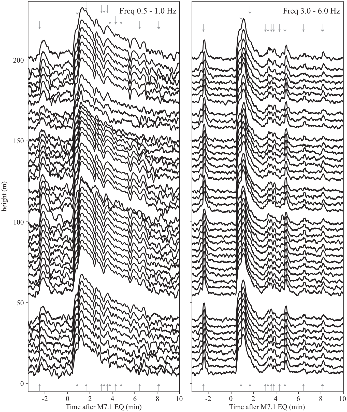
Frequency-dependent log-amplitude of shaking due to the M7.1 Ridgecrest earthquake, foreshock, and aftershocks with M > 4.5 for all sensors. Arrows mark the expected arrival time of the S-wave for all earthquakes. Note how at low frequencies (left panel), the shaking due to the M7.1 earthquake overwhelms the shaking of the aftershocks, but at higher frequencies (3–6 Hz, higher modes) (right panel), the shaking of the M7.1 earthquake is quickly damped and the shaking for small aftershocks can readily be observed.

Figure 11.

Damping estimates (see Figure 9) and amplitude of shaking (log envelope, Figure 10) at low and high frequencies showing how damping modulation is strongly influenced by shaking due to smaller aftershocks at high frequencies, while not so much at low frequencies.

This could explain why the small-amplitude foreshock and aftershocks have a relatively large effect on the damping ratios immediately after those earthquake motions impact the building; the foreshock and aftershock effects are nearly as large as the M7.1 mainshock. Self-similarity laws for earthquake sources, in which the moment is a function of the cube root of corner frequency in the source spectrum, suggest that smaller-moment foreshocks and aftershocks will have larger corner frequencies than the mainshock (Aki, 1967; Prieto et al., 2004). This could result in larger-than-expected impact of smaller-magnitude earthquakes on the higher modes of the high-rise in downtown Los Angeles.

Friction may occur when elements or surfaces come into contact and move relative to each other during shaking. Such changes in friction properties, and the kinetic energy associated with the relative motions and impacts, may lead to thermal energy production and energy loss, and thus short-term damping increases. The building’s non-structural elements likely contribute relative motion on small spatial scales (e.g. one floor) during the strong shaking in the same way that relative motion on small pre-existing cracks in a building may be temporarily activated during strong shaking. A similar slow recovery process after strong shaking was observed for aftershocks of the 2011 Tohoku earthquake and is interpreted as the healing of cracks (Astorga and Guéguen, 2020). For example, discontinuities or separations in non-structural partition walls may cause relative motion in the partition wall relative to the main structural wall, and relative motion in one section of the partition wall relative to another section. With these types of mechanisms, overall stiffness is, in addition, reduced during shaking. The small scale of friction-damping sources is consistent with our observation of higher frequencies predominating the damping ratio changes.

Conclusion

A coda wave seismic interferometric technique (CWI) is applied to the acceleration waveform data recorded in a steel moment-and-brace frame high-rise in downtown Los Angeles that recorded the 2019 Ridgecrest earthquake sequence. The accelerations are recorded continuously (24/7/365) at 50 sps on a dense MEMS-based strong-motion array operated by the CSN. The waveform data are analyzed for time periods during shaking from the M7.1 Ridgecrest mainshock, as well as aftershocks and a foreshock. These are compared with ambient vibrations recorded on days that exhibited no significant seismicity. A cross-correlation method is applied to the pairs of data consisting of the second floor and every other floor above and below it, to obtain the time-domain IRFs. Broadband shear-wave velocities are reduced by as much as 10% during building shaking due to the Ridgecrest sequence, and their restoration to pre-earthquake levels is found to be a function of the decrease in shaking amplitude levels over a broad frequency band. The temporal variations of the IRF can be resolved over time scales of tens of seconds and on a spatial scale that depends on station density, throughout the entire duration of the building shaking. Damping ratios measured over narrow frequency bands increase significantly over short time durations spanning the main shock, and M > 4.5 aftershocks and a foreshock. The largest damping ratio increases occur for the highest frequencies, and the increase is attributed to friction associated with structural and non-structural surface discontinuities which experience relative motion and impact during shaking, resulting in energy loss. The damping ratio measurement represents an average over all floors.

Until recently, CWI techniques have been limited by sparsity of measurements or short-term sensor deployments inside buildings, both of which limit the spatial and temporal resolution of possible changes in properties due to damage or nonlinear inelastic response. The benefits of this approach to SHM are that: it is a non-parameterized mathematical approach that does not depend on modal identification, structure type or geometry, structural materials, or similar a priori assumptions; it couples nonlinear response characterization together with the underlying physics of deformation; it can map nonlinear response characterization; and it could comprise an automated real-time system identification and damage detection method that can potentially be applied to the rapidly growing field of permanent, continuously recording sensor networks—all of which with spatial resolution dependent on station density. This method illustrates a way to compute higher-frequency damping (and its temporal variations), even if the building’s resonant frequencies are not known or are uncertain.

The results from this earthquake and ambient vibration analysis suggest that monitoring a structural system’s IRFs from continuous waveform data is observable in the presence of dense, low-cost sensor array data, and that changes in the propagating wave properties can be resolved to make interpretations of dynamic building response and, potentially, damage. If small-scale permanent damage has occurred by a physical mechanism, for example, a fracture in a beam flange, that will affect the system’s inelastic properties and density, then those changes could be observable in continuous IRFs. In addition, interferometric techniques that include coda waves to monitor structural health should also be able to resolve geometric nonlinearities since they will also impact IRF properties when the sampling lengths (sensor spacing) are appropriately small.

Supplemental Material

sj-docx-1-eqs-10.1177_87552930241240458 – Supplemental material for Time-varying damping ratios and velocities in a high-rise during earthquakes and ambient vibrations from coda wave interferometry

Supplemental material, sj-docx-1-eqs-10.1177_87552930241240458 for Time-varying damping ratios and velocities in a high-rise during earthquakes and ambient vibrations from coda wave interferometry by Germán A Prieto and Monica D Kohler in Earthquake Spectra

Footnotes

Acknowledgements

The authors thank Jonathan Stewart, Tom Heaton, Chen Ji, and Philippe Gueguen for discussions on this topic prior to publication. M.D.K. thanks Gabriel Pizarro for computer hardware and software support directly related to this project.

Declaration of conflicting interests

The author(s) declared no potential conflicts of interest with respect to the research, authorship, and/or publication of this article.

Funding

The author(s) disclosed receipt of the following financial support for the research, authorship, and/or publication of this article: The Community Seismic Network (CSN) was supported by Caltech, the Conrad N. Hilton Foundation, and Computers and Structures, Inc.

ORCID iD

Germán A Prieto

Data and resources

Community Seismic Network (CSN) strong-motion data for the 2019 Ridgecrest earthquake are available from .

Supplemental material

Supplemental material for this article is available online.

References

Abazarsa

Nateghi

Ghahari

Taciroglu

(2013) Blind modal identification of non-classically damped systems from free or ambient vibration records. Earthquake Spectra 29(4): 1137–1157.

Aki

(1967) Scaling law of seismic spectrum. Journal of Geophysical Research 72(4): 1217–1231.

Astorga

Guéguen

(2020) Structural health building response induced by earthquakes: Material softening and recovery. Engineering Reports 2(9): e12228.

Bernal

Döhler

Kojidi

Kwan

Liu

(2015) First mode damping ratios for buildings. Earthquake Spectra 31(1): 367–381.

Bernal

Mozaffari

Kwan

Döhler

(2012) Damping identification in buildings from earthquake records. SMIP seminar on utilization of strong motion data proceedings. Available at: https://www.conservation.ca.gov/cgs/pages/program-smi/seminar/smip12_toc.aspx (March 2024).

Brenguier

Campillo

Hadziioannou

Shapiro

Nadeau

Larose

(2008a) Postseismic relaxation along the San Andreas fault at parkfield from continuous seismological observations. Science 321: 1478–1481.

Brenguier

Shapiro

Campillo

Ferrazzini

Duputel

Coutant

Nercessian

(2008b) Towards forecasting volcanic eruptions using seismic noise. Nature Geoscience 1(2): 126–130.

Celebi

Kashima

Ghahari

Koyama

Taciroglu

Okawa

(2017) Before and after retrofit behavior and performance of a 55-story tall building inferred from distant earthquake and ambient vibration data. Earthquake Spectra 33(4): 1599–1626.

Celebi

Ulusoy

Nakata

(2016) Responses of a tall building in Los Angeles, California, as inferred from local and distant earthquakes. Earthquake Spectra 32: 1821–1843.

10.

Clayton

Heaton

Kohler

Chandy

Guy

Bunn

(2015) Community seismic network: A dense array to sense earthquake strong motions. Seismological Research Letters 86: 1354–1363.

11.

Clayton

Kohler

Guy

Bunn

Heaton

Chandy

(2020) CSN/LAUSD network: A dense accelerometer network in Los Angeles Schools. Seismological Research Letters 91(2A): 622–630.

12.

Clinton

Bradford

Heaton

Favela

(2006) The observed wander of the natural frequencies in a structure. Bulletin of the Seismological Society of America 96: 237–257.

13.

Desmond

Valenza

(2019) Sensitivity of coda wave interferometry to fluid migration through rock. The Journal of the Acoustical Society of America 145(2): 1100–1104.

14.

Ebrahimian

Kohler

Massari

Asimaki

(2018) Parametric estimation of dispersive viscoelastic layered media with application to structural health monitoring. Soil Dynamics and Earthquake Engineering 105: 204–223.

15.

Ebrahimian

Todorovska

(2014) Wave propagation in a Timoshenko beam building model. Journal of Engineering Mechanics 140: 04014018.

16.

Ebrahimian

Todorovska

(2015) Structural system identification of buildings by a wave method based on a nonuniform Timoshenko Beam model. Journal of Engineering Mechanics 141(8): 04015022.

17.

Fröjd

Ulriksen

(2017) Frequency selection for coda wave interferometry in concrete structures. Ultrasonics 80: 1–8.

18.

Ghahari

Abazarsa

Taciroglu

(2016) Blind modal identification of non-classically damped structures under non-stationary excitations. Structural Control and Health Monitoring 24(6): e1925.

19.

Ghahari

Abazarsa

Ghannad

Taciroglu

(2012) Response-only modal identification of structures using strong motion data. Earthquake Spectra 42(8): 1221–1242.

20.

Goel

Chopra

(1997) Vibration properties of buildings determined from recorded earthquake motions. Report no. UCB/EERC-97/14, December. Berkeley, CA: Earthquake Engineering Research Center, University of California.

21.

Grêt

Snieder

Aster

Kyle

(2005) Monitoring rapid temporal change in a volcano with coda wave interferometry. Geophysical Research Letters 32(6): L06304.

22.

Hadziioannou

Larose

Coutant

Roux

Campillo

(2009) Stability of monitoring weak changes in multiply scattering media with ambient noise correlation: Laboratory experiments. The Journal of the Acoustical Society of America 125(6): 3688–3695.

23.

Hart

Vasudevan

(1975) Earthquake design of buildings: Damping. Journal of the Structural Division 101(1): 11–30.

24.

Hudson

(1965) Equivalent viscous friction for hysteretic systems with earthquake-like excitations. In: Proceedings of the 3rd world conference on earthquake engineering, Wellington, New Zealand, 22 January–1 February, Vol. 11, pp. 185–201. Wellington, New Zealand: New Zealand National Committee on Earthquake Engineering.

25.

Jacobsen

(1930) Steady forced vibration as influenced by damping. Transactions of the American Society of Mechanical Engineers 52: 169–178.

26.

Jacobsen

(1960) Damping in composite structures. In: Proceedings of the 2nd world conference on earthquake engineering, Tokyo and Kyoto, Japan, 11–18 July, Science Council of Japan, pp. 1029–1044.

27.

Jaimes

Prieto

Rodriguez

(2022) Detection of building response changes using deconvolution interferometry: A case study in Bogota, Colombia. Seismological Research Letters 93(2A): 931–942.

28.

Jeary

(1992) Establishing non-linear damping characteristics of structures from non-stationary response time-histories. The Structural Engineer 70(4): 61–66.

29.

Jeary

Ellis

(1984) Non-destructive in situ testing using dynamics techniques. In: Proceedings of the 3rd international conference on tall buildings, Hong Kong and Guangzhou, China, December, CTBUH, pp. 76–81.

30.

Kashima

(2017) Study on changes in dynamic characteristics of high-rise steel-framed buildings based on strong motion data. Procediaengineering 199: 194–199.

31.

Kashima

Koyama

Iiba

Okawa

(2014) Change in dynamic characteristics of RC/SRC buildings during the 2011 Great East Japan Earthquake. In: Proceedings of the 10th national conference earthquake engineering, Anchorage, AK, 21–25 July.

32.

Kohler

Filippitzis

Heaton

Clayton

Guy

Bunn

Chandy

(2020) 2019 Ridgecrest earthquake reveals areas of Los Angeles that amplify shaking of high-rises. Seismological Research Letters 91(6): 3370–3380.

33.

Kohler

Heaton

Bradford

(2007) Propagating waves recorded in the steel, moment-frame Factor Building during earthquakes. Bulletin of the Seismological Society of America 97: 1334–1345.

34.

Kohler

Heaton

Cheng

Singh

(2014) Structural health monitoring through dense instrumentation by community participants: The Community Seismic Network and Quake-Catcher Network. In: 10th U.S. National conference on earthquake engineering (NC10EE), Anchorage, AK, 21–25 July.

35.

Kohler

Massari

Heaton

Kanamori

Hauksson

Guy

Chandy

(2016) Downtown Los Angeles 52-story high-rise and free-field response to an oil refinery explosion. Earthquake Spectra 32(3): 1793–1820.

36.

Lagomarsino

(1993) Forecast models for damping and vibration periods of buildings. Journal of Wind Engineering and Industrial Aerodynamics 48(2–3): 221–239.

37.

McVerry

(1979) Frequency domain identification of structural models from earthquake records. EERL report no. 79-027902, October. Pasadena, CA: California Institute of Technology. Available at: https://resolver.caltech.edu/CaltechEERL:1979.EERL-79-02 (March 2024).

38.

McVerry

(1980) Structural identification in the frequency domain from earthquake records. Earthquake Engineering and Structural Dynamics 8: 161–180.

39.

Miranda

Cruz

(2017) Damping ratios in tall buildings inferred from instrumented tall buildings in California. In: International workshop on performance-based seismic design of structures (PESDES), Shanghai, China, 13–15 October.

40.

Mordret

Mikesell

Harig

Lipovsky

Prieto

(2016) Monitoring southwest Greenland’s ice sheet melt with ambient seismic noise. Science Advances 2(5): e1501538.

41.

Mordret

Sun

Prieto

Toksöz

Büyüköztürk

(2017) Continuous monitoring of high-rise buildings using seismic interferometry. Bulletin of the Seismological Society of America 107(6): 2759–2773.

42.

Nakata

Snieder

(2011) Near-surface weakening in Japan after the 2011 Tohoku-Oki earthquake. Geophysical Research Letters 38: L17302.

43.

Nakata

Snieder

(2014) Monitoring a building using deconvolution interferometry. II: Ambient vibration analysis. Bulletin of the Seismological Society of America 104(1): 204–213.

44.

Nakata

Snieder

Kuroda

Ito

Aizawa

Kunimi

(2013) Monitoring a building using deconvolution interferometry, I: Earthquake-data analysis. Bulletin of the Seismological Society of America 103(3): 1662–1678.

45.

Peng

Ben-Zion

(2006) Temporal changes of shallow seismic velocity around the Karadere-Duzce branch of the North Anatolian Fault and strong ground motion. Pure and Applied Geophysics 163: 567–600.

46.

Planès

Larose

(2013) A review of ultrasonic Coda Wave Interferometry in concrete. Cement and Concrete Research 53: 248–255.

47.

Poupinet

Ellsworth

Frechet

(1984) Monitoring velocity variations in the crust using earthquake doublets: An application to the Calaveras Fault, California. Journal of Geophysical Research: Solid Earth 89(B7): 5719–5731.

48.

Prieto

(2022) The multitaper spectrum analysis package in Python. Seismological Society of America 93(3): 1922–1929.

49.

Prieto

Lawrence

Chung

Kohler

(2010) Impulse response of civil structures from ambient noise analysis. Bulletin of the Seismological Society of America 100(5A): 2322–2328.

50.

Prieto

Shearer

Vernon

Kilb

(2004) Earthquake source scaling and self-similarity estimation from stacking P and S spectra. Journal of Geophysical Research: Solid Earth 109(B8): B08310.

51.

Rahmani

Todorovska

(2021) Structural health monitoring of a 32-story steel moment-resisting frame building using 50 years of seismic monitoring data. Earthquake Engineering & Structural Dynamics 50(6): 1777–1800. https://doi.org/10.1002/eqe.3422

52.

Rahmani

Ebrahimian

Todorovska

(2015) Time-wave velocity analysis for early earthquake damage detection in buildings: Application to a damaged full-scale RC building. Earthquake Engineering & Structural Dynamics 44(4): 619—636.

53.

Rahmani

Hao

T-Y

Todorovska

Boroschek

(2017) Structural health monitoring of Torre Central by the wave method. In: 16th world conference on earthquake engineering, Santiago, Chile, 9–13 January, Paper no. 3651. Kanpur, India: National Information Centre of Earthquake Engineering.

54.

Reinoso

Miranda

(2005) Estimation of floor acceleration demands in highrise buildings during earthquakes. The Structural Design of Tall and Special Buildings 14(2): 107–130.

55.

Ross

Idini

Jia

Stephenson

Zhong

Wang

Zhan

Simons

Fielding

E. J

Yun

S-H

Hauksson

Moore

Liu

Jung

(2019) Hierarchical interlocked orthogonal faulting in the 2019 Ridgecrest earthquake sequence. Science 366(6463): 346–351.

56.

Rubinstein

Beroza

(2004a) Evidence for widespread nonlinear strong motion in the MW 6.9 Loma Prieta earthquake. Bulletin of the Seismological Society of America 94: 1595–1608.

57.

Rubinstein

Beroza

(2004b) Nonlinear strong ground motion in the ML 5.4 Chattenden earthquake: Evidence that preexisting damage increases susceptibility to further damage. Geophysical Research Letters 31: L23614.

58.

Satake

Suda

Arakawa

Sasaki

Tamura

(2003) Damping evaluation using full-scale data of buildings in Japan. Journal of Structural Engineering 129(4): 470–477.

59.

Sawazaki

Sato

Nakahara

Mishimura

(2006) Temporal change in site response caused by earthquake strong motion as revealed from coda spectral ratio measurement. Geophysical Research Letters 33: L21303.

60.

Sens-Schönfelder

Wegler

(2006) Passive image interferometry and seasonal variations of seismic velocities at Merapi Volcano, Indonesia. Geophysical Research Letters 33(21): L21302.

61.

Serra

Festa

Vassallo

Zollo

Quattrone

Ceravolo

(2017) Damage detection in elastic properties of masonry bridges using coda wave interferometry. Structural Control and Health Monitoring 24(10): e1976.

62.

Sheng

Mordret

Sager

Brenguier

Boué

Rousset

Vernon

Higueret

(2022) Monitoring seismic velocity changes across the San Jacinto fault using train-generated seismic tremors. Geophysical Research Letters 49(19): e2022GL098509.

63.

Snieder

(2006) The theory of coda wave interferometry. Pure and Applied Geophysics 163(2): 455–473.

64.

Snieder

Safak

(2006) Extracting the building response using interferometric imaging; Theory and application to the Millikan Library in Pasadena, California. Bulletin of the Seismological Society of America 96: 586–598.

65.

Snieder

Grêt

Douma

Scales

(2002) Coda wave interferometry for estimating nonlinear behavior in seismic velocity. Science 295(5563): 2253–2255.

66.

Soroka

(1949) Note on the relations between viscous and structural damping coefficients. Journal of the Aeronautical Sciences 16(7): 409–410.

67.

Stähler

Sens-Schönfelder

Niederleithinger

(2011) Monitoring stress changes in a concrete bridge with coda wave interferometry. The Journal of the Acoustical Society of America 129(4): 1945–1952.

68.

Sun

Mordret

Prieto

Toksöz

Büyüköztürk

(2017) Bayesian characterization of buildings using seismic interferometry on ambient vibrations. Mechanical Systems and Signal Processing 85: 468–486.

69.

Tamura

Suganuma

(1996) Evaluation of amplitude-dependent damping and natural frequency of buildings during strong winds. Journal of Wind Engineering and Industrial Aerodynamics 59: 115–130.

70.

Taranath

(1997) Steel, Concrete, and Composite Design of Tall Buildings. 2nd ed. San Francisco, CA: McGraw-Hill.

71.

Todorovska

Trifunac

(2008a) Earthquake damage detection in the Imperial County Services Building III: Analysis of wave travel times via impulse response functions. Soil Dynamics and Earthquake Engineering 28(5): 387–404.

72.

Todorovska

Trifunac

(2008b) Impulse response analysis of the Van Nuys 7-storey hotel during 11 earthquakes and earthquake damage detection. Structural Control and Health Monitoring 15(1): 90–116.

73.

Wang

Niederleithinger

Hindersmann

(2022) The installation of embedded ultrasonic transducers inside a bridge to monitor temperature and load influence using coda wave interferometry technique. Structural Health Monitoring 21(3): 913–927.

74.

Zhang

Cho

(2009) Experimental study on damping ratios of in-situ buildings. International Journal of Mechanical and Mechatronics Engineering 3(2): 191–195.

Supplementary Material

Please find the following supplemental material available below.

For Open Access articles published under a Creative Commons License, all supplemental material carries the same license as the article it is associated with.

For non-Open Access articles published, all supplemental material carries a non-exclusive license, and permission requests for re-use of supplemental material or any part of supplemental material shall be sent directly to the copyright owner as specified in the copyright notice associated with the article.

0.00 MB

1.43 MB