Efficient incorporation of rupture directivity into probabilistic seismic hazard analysis using a deep learning

Abstract

Earthquakes with rupture forward directivity effects can produce high amplitude, pulse-like ground shaking, which imposes significantly greater seismic demands on buildings compared to non-pulse-like shaking of similar amplitude. Although theoretical frameworks exist for the incorporation of rupture directivity effects into probabilistic seismic hazard analysis (PSHA), the associated computational burden often makes it impractical for regional-scale studies in practice. Furthermore, many available models to estimate directivity are limited to the application to ruptures of limited geometrical complexity. In this study, we develop a deep learning–based model that provides adjustment terms (moment modifiers) for the mean and standard deviation of ground motion distributions near an earthquake rupture, as predicted by a ground motion model. Thereby the model depends on a chosen distribution of hypocenters along the fault, but not on individual hypocenter locations. Our model is trained on a synthetic dataset generated from an empirical directivity amplification model that includes a wide variety of earthquake ruptures, encompassing diverse seismic properties such as magnitude, dip angle, and faulting style, as well as geometrical complexities ranging from simple, planar ruptures to intricate, multi-segment, branching ruptures with step-overs and strike reversals. This enables our model to provide accurate moment modifiers for a broad spectrum of earthquake ruptures in PSHA and other applications like scenario-based estimates of shaking and loss. The final model can be easily integrated into existing seismic hazard frameworks, as demonstrated by an application in a complete PSHA calculation for Turkey. The results indicate that explicitly incorporating directivity effects can lead to significant changes in long period seismic hazard, and through the use of efficient moment modifier models based on deep learning it can be possible to expand the usage of directivity models in seismic hazard and risk analysis at large regional scales.

Keywords

Probabilistic seismic hazard analysis rupture directivity modeling deep learning

Introduction

The term rupture forward directivity describes the generation of high-amplitude ground motion with a short duration that can occur in the near-fault area of large earthquake ruptures. Such pulse-like ground motion is caused if an earthquake rupture propagates at a velocity close to the shear wave velocity of the surrounding medium, and if the direction of slip is aligned with the observation site (Somerville et al., 1997). Somerville (2003) has shown empirically that directivity affects only a narrow frequency band, where the peak period depends on the magnitude of the earthquake source. This empirical observation was moreover linked to physical properties such as the rise-time and the source dimensions, which generally increase with earthquake magnitude. Rupture forward directivity (directivity hereafter) has been observed for several earthquakes in the past, such as the 1992 $M_{W} 7.3$ Landers, California (Wald and Heaton 1994), 1999 $M_{W} 7.6$ Chi-Chi, Taiwan (Xie 2019), 2010 $M_{W} 7.1$ Darfield, New Zealand (Bradley et al., 2014), and the 2023 $M_{W} 7.6$ and $M_{W} 7.8$ Kahramanmaraş, Türkiye (Mai et al., 2023) earthquakes. The resulting pulse-like ground motions from forward directivity can impose larger seismic demands on engineered structures than non-pulse-like motions of similar amplitude (Bertero et al., 1978; Hall et al., 1995; Mavroeidis et al., 2004).

Despite its relevance for engineering applications, explicit incorporation of directivity effects in ground motion modeling and probabilistic seismic hazard analysis (PSHA) has not yet become firmly established. Instead, it is typically captured implicitly during the regression stage of ground motion model (GMM) development, simply due to the fact that an often unspecified fraction of observations is affected by directivity. Because the pulse-like characteristics of directivity relevant to PSHA diminishes quickly beyond the near-field region, and because aleatory uncertainty is typically not treated distance dependent in most GMMs, this procedure leads to an underestimation of ground motion variability at short source-to-site distances and overestimation at greater distances (Abrahamson, 2000), and can fail to capture strong azimuthal variations in mean and variability that may occur in the near-fault region.

Although considerable efforts have been undertaken to overcome this issue via the explicit incorporation of directivity effects in ground motion modeling (summarized in Spudich et al., 2013), to date the GMM of Chiou and Youngs (2014) is the only one to include an explicit directivity term. As an alternative, directivity adjustment models, such as the one from Somerville et al. (1997), later updated in Abrahamson (2000), or Bayless et al. (2020) and Bayless et al. (2024), are inferred from ground motion residuals of directivity neutral GMMs in order to provide post hoc adjustments of GMM predictions. However, such directivity adjustment models usually depend on the exact hypocenter location on a rupture plane, such that an additional computational loop over various hypocenter locations would have to be added to PSHA calculation workflows. This full hypocenter randomization approach is realizable for earthquake source models of limited size and complexity, as shown by the implementation for the 2010 New Zealand National Seismic Hazard Model (NSHM) (Stirling et al., 2012) by Weatherill and Lilienkamp (2023), but the associated computational effort becomes disproportionally large for large scale PSHA calculations for state-of-the-art source models such as the one presented in Seebeck et al. (2023) and Van Dissen et al. (2022) for the 2022 New Zealand NSHM (Gerstenberger et al., 2022a, 2022b), or the Uniform California Earthquake Rupture Forecast version 3 (UCERF v.3) (Field et al., 2014; Page et al., 2014) as recently shown by the implementation of the full hypocenter randomization approach by Al Atik et al. (2023).

As an alternative to the full hypocenter randomization approach, Watson-Lamprey (2018) suggests to modify the moments of the probability distribution of ground motion that is predicted by a directivity neutral GMM (median and variance) with adjustment terms that account for the average directivity effect according to a predefined spatial distribution of hypocenter locations on a rupture plane. These so-called modifiers of moments are consequently hypocenter location independent and can therefore be incorporated with little computational effort in large-scale PSHA computations (Donahue et al., 2019).

To implement such a model, Watson-Lamprey (2018) suggests to fit empirical, closed-form equations to synthetically calculated moment modifiers. Although this approach is computationally efficient, a loss of accuracy compared to the synthetic moment modifiers is ascertained, which is caused by the relatively simple parametric form of the chosen equation. The severity of this issue is acceptable for the simple ruptures the model was calibrated with, and a certain stretch toward slightly more complex ruptures is also within reach as recently demonstrated by Withers et al. (2024b). However, the ascertained limitation in reproducing the finer details of the moment modifier fields in such cases raises doubts regarding the applicability of such a model to highly complex, branching multi-segment ruptures as they can occur in advanced source models. Kelly et al. (2022) and Withers et al. (2024a) are addressing this limitation following an approach in which they use a shallow artificial neural network (ANN) approach to predict point-wise values of moment modifiers for a wide range of rupture geometries and seismic properties from a subset of simple ruptures from UCERF v.3.

A similar approach was suggested by Weatherill and Lilienkamp (2023) who utilize a convolutional artificial neural network (ANN) to efficiently and accurately generate maps of moment modifiers for 3884 complex, multi-segment earthquake ruptures from the 2022 New Zealand NSHM. However, in this case the objective was to define a compact representation of the directivity fields specifically for the ruptures contained within the New Zealand NSHM. Therefore, the resulting model is not capable of generalizing to ruptures beyond those contained within the 2020 New Zealand NSHM rupture inventory.

The purpose of this study is to modify this ANN approach in order to derive a deep learning model that generalizes to a wide range of rupture geometries and seismic properties. Critically, to facilitate its use in PSHA the model takes as predictors parameters that are already adopted by existing ground motion models, and thus would not require the adaptation of the calculation software to compute new source and path parameters. Doing so can facilitate wider usage of the neural network model to different regions of the world and to different types of seismogenic fault source models. The study is organized as follows: In the next section, we will introduce the adapted modifier of moments approach, followed by a brief description of the generated synthetic data set. A detailed description of the model calibration procedure using the U-Net neural network architecture (Ronneberger et al., 2015) and some modeling results are presented thereafter. Subsequently we present a practical application of the derived model in a PSHA calculation for Turkey. We finalize the study with a brief discussion of the model performance and some advice for practical usage.

The modifier of moments approach

The modifier of moments approach (Watson-Lamprey, 2018) is a means of directly including directivity effects in the seismic hazard integral (Equation 1, Cornell, 1968), without the need for an additional integral to account for hypocenter location uncertainty, which would significantly increase computational demand (Donahue et al., 2019).

λ (Y \geq y ∣ T) = \sum_{i = 1}^{N_{SRCS}} λ_{m > M_{\min}, i} \int_{M} \int_{R} P [Y \geq y | m, r, T, θ_{dir}, f_{H}] \cdot f_{M_{i}} (m) \cdot f_{R, i} (r ∣ m) dr dm

(1)

Here, $λ$ represents the rate at which a ground motion intensity measure $Y$ at response period $T$ exceeds or equals level $y$ at a site. $N_{SRCS}$ is the number of earthquake sources capable of generating significant ground motion at the site, and $λ_{m > M_{\min}, i}$ is the rate at which the magnitude $m$ of the $i$ th source exceeds its minimum considered magnitude $M_{\min}$ . $P [Y \geq y | m, r, T, θ_{dir}, f_{H}]$ is the probability of ground motion level $y$ being exceeded in a specific earthquake scenario, where $θ_{dir}$ represents the parameters used to model directivity-related amplification, and $f_{H}$ denotes the spatial distribution of hypocenter locations on a rupture surface. $f_{M_{i}} (m)$ represents the magnitude distribution of the $i$ th source, and $f_{R, i} (r | m)$ describes the source-to-site distance distribution for an earthquake of a given magnitude at the $i$ th source.

The term:

\begin{matrix} P [Y \geq y | m, r, T, θ_{dir}, f_{H}] = \\ 1 - \int_{- \infty}^{y} \frac{1}{σ^{'} (θ_{dir} | f_{H}) \sqrt{2 π}} \exp [- \frac{1}{2} {(\frac{Y - [μ (m, r, T) + \bar{Δ μ_{dir}} (θ_{dir} | f_{H})]}{σ^{'} (θ_{dir} | f_{H})})}^{2}] dY, \end{matrix}

(2)

where

{σ^{'}}^{2} (θ_{dir} | f_{H}) = σ^{2} (T) + Δ σ_{red}^{2} (T) + {\bar{Δ σ_{dir}}}^{2} (θ_{dir} | f_{H}),

(3)

is typically solved using a GMM, which considers the logarithm of a ground motion intensity measure to be normally distributed with median $μ (m, r, T)$ and variance $σ^{2} (T)$ (the moments of the normal distribution). The moment modifiers $\bar{Δ μ_{dir}} (θ_{dir} | f_{H})$ and $\bar{Δ σ_{dir}} (θ_{dir} | f_{H})$ then adjust the GMM moments to account for directivity effects given the distribution of hypocenter locations on the fault $f_{H}$ . The adjustment to the total aleatory variability described by the term on the far right of Equation 3 applies only to the moment modifier models. The adjustment term $Δ σ_{red}^{2}$ accounts for the reduction of the aleatory variability of the GMM due to the change of incorporating directivity explicitly in the median instead of considering it a random perturbance of ground motion (Bayless et al., 2020).

Data

The first step toward a universally applicable, ANN based modifier of moments model is the generation of a large and diverse synthetic data set. This data set must contain $N_{rup}$ representations of earthquake ruptures (predictive parameters $X$ ), and the corresponding moment modifiers $\bar{Δ μ_{dir}}$ and $\bar{Δ σ_{dir}}$ (target parameters $Y$ ). As outlined in the Introduction, the amplitude of directivity related amplification depends on the earthquake’s magnitude $M$ , the response period $T$ , and the alignment of an observation site with the direction of slip on the rupture. For the latter condition, the style of faulting ( $SOF$ ) and a 3D mesh of coordinates describing the rupture surface could be utilized to represent an earthquake rupture. However, since the meshes for different earthquake ruptures usually vary substantially, it is difficult to make such a representation compatible with the fixed-size input layer of a neural network. Therefore, we decided to not use the 3D rupture geometry itself, but various source-to-site distance metrics derived from the rupture as predictive input parameters. In total, we consider 8 predictive parameters $θ_{dir}$ : Magnitude $M$ , response period $T (s) \in$ {0.75, 1.00, 1.25, 1.50, 2.00, 2.50, 3.00, 4.00, 5.00, 7.50, 10.00}, rupture plane distance $R_{rup}$ , Joyner-Boore distance $R_{jb}$ , the along-strike horizontal distance of a site to the rupture $R_{y 0}$ , coordinates $GC 2_{t}$ and $GC 2_{u}$ (according to the generalized coordinate system 2 (Spudich and Chiou, 2015), and the style of faulting $SOF \in$ {0, 1} (dip-slip $\hat{=}$ 0, strike-slip $\hat{=} 1$ , respectively). The latter six parameters thereby describe the alignment of a site with the slip direction on the rupture. While the usage of five different distance metrics leads to considerable redundancy in the input information, the nuanced difference between the distance metrics enable a very precise description of the rupture geometry at short distances. We emphasize at this point that our selection of predictive parameters is tailored to the Bayless et al. (2020) directivity model, which we use for the generation of our synthetic data set. If a different directivity adjustment model is used during data generation, a different composition of input parameters according to this model may be advised.

In order to describe earthquake ruptures of various sizes, shapes, and complexities in a standardized way for usage in a deep learning model, we decided to format the predictive parameters for each rupture $x_{i} i \in {1, \dots, N_{rup} \cdot N_{T}}$ where $N_{T} = 11$ is the number of considered response periods, via a set of maps (rasters) of size 256×256 with a spacing of 5 km. Although magnitude, style of faulting, and response period could actually be described by single numbers, we represent those parameters as arrays with the same geometry as the distance metrics (assigning the same value to each pixel) to make them compatible with the ANN architecture.

To calculate the moment modifiers $y_{i}$ , we assume a given distribution of hypocenter positions within the rupture ( $f_{H}$ ), from which we draw 250 sample hypocenters per rupture using the two-step sampling procedure from Weatherill and Lilienkamp (2023). For hypocenter along-strike position, we adopt the preferred probability mass functions proposed by Watson-Lamprey (2018). For strike-slip ruptures, this describes a symmetric distribution with 0.5 of the total weight distributed uniformly for hypocentres located in bins of 0.1 between 0.3 and 0.7 of the total rupture length, 0.25 of the total weight distributed uniformly between 0 and 0.2 of the total rupture length, and 0.25 to distributed uniformly between 0.8 to 1.0 of the total rupture length (see Figure 3 of Weatherill and Lilienkamp (2023)). In this manner, bilateral and unilateral propagating ruptures are weighted evenly. For dip-slip ruptures, a normal distribution is assumed with the highest weights given to hypocenter positions in the middle of the rupture length. For down-dip hypocenter position, we use the model of Melgar and Hayes (2019) that describes a Gaussian distribution $N (μ = 0.55, σ = 0.2)$ , which is adapted and re-normalized so that it is truncated in the range [0, 1]. This continuous distribution then discretized into three bins for strike-slip ruptures and five bins for dip-slip ruptures using the Gaussian Quadrature approximation approach of Miller and Rice (1983). The two-step sampling approach first samples the discrete bin for the hypocenter position according to the bin weights, then in the second step the final hypocenter position is sampled uniformly within the bin in order to establish a smoother distribution of hypocenters across the fault.

According to the criteria for the selection of an appropriate directivity model suggested in Weatherill and Lilienkamp (2023), we select the Bayless et al. (2020) model to simulate the directivity amplification patterns for each hypocenter location. This model is particularly well suited for application to ruptures of increasing complexity, as the azimuthal component of the directivity predictor itself adopts the GC2 framework that aims to ensure a topologically continuous representation of fault normal and fault parallel distances even in cases where faults may contain topological discontinuities such as gaps or step-overs. This makes it computationally efficient and facilitates integration into many PSHA software codes where functions to calculate GC2 are already present. Bayless et al. (2020) is also calibrated using ground motions from observed earthquakes with complex multi-segment ruptures, complemented with data from physics-based simulations, meaning that complex ruptures are well represented in the underlying dataset. In a final step, we average over the $N_{SAMP}$ = 250 amplification fields to obtain maps of the moment modifiers ${\bar{Δ μ}}_{dir}$ and $\bar{Δ σ_{dir}}$ . A supporting illustration regarding the data generation procedure is given in the supplemental material S1 to this article.

To enable the best possible generalization to arbitrary earthquake ruptures of the final model, we need to ensure that the training data set encompasses a large variety of different earthquake ruptures, both in terms of seismic properties such as magnitude, strike-angle, and dip-angle, but also in terms of geometrical complexity. To this end we include three different earthquake rupture forecasts (NZ—New Zealand Community Fault Model (Seebeck et al., 2023), TUR—Turkey Fault Model (Basili et al., 2024; Danciu et al., 2021), GEN—A generic inventory of simple planar ruptures) in the synthetic dataset.

The NZ model is characterized by a large amount of branching, multi-segment ruptures including complexities such as step-overs and reversals of dip direction between segments. Out of the 3884 ruptures in the inventory, we reject 227 due to issues with the calculation of $GC 2$ coordinates or the contribution from multiple faults with significantly different $SOF$ , a feature that our model does not support. We split the remaining ruptures into a training set (2849) used for optimizing the ANN model, and a validation set (808) used for verification that the model generalizes to previously unseen ruptures. Because many ruptures in the ERF share a large number of common segments, a simple random split seems insufficient in order to cleanly separate the training and the validation sets. Therefore, we quantify the similarity of ruptures as the fraction of shared segments and subsequently apply multi-dimensional scaling (MDS) to identify clusters of ruptures with high similarity. Separation into the training and validation sets is then performed visually using the MDS results, ensuring that highly similar ruptures end up together in either the training or the validation data set.

The TUR inventory is composed of multi-segment ruptures that are topologically simpler compared to those from the NZ model. These ruptures allow for changes in strike along length, but the dip and style-of-faulting are constant and the segments are connected only at the segment ends (i.e. without offsets and step-overs). The ruptures are generated from the ESHM20 fault source model (Basili et al., 2024), whose full ERF is modeled with a truncated Gutenberg-Richter distribution between $M_{W} 5.75$ and $M_{W} 8.5$ . To avoid oversampling the smaller magnitude ruptures, we sort the complete ERF into bins of 0.5 $M_{W}$ and draw no more than 100 sample ruptures from each bin if the bin contains more than 100 ruptures (for larger magnitudes all the ruptures in the bin were retained. We apply the same MDS based split strategy of the 1929 ruptures into a training (1528) and a validation (401) set. A summary of the split procedures for the NZ and TUR rupture inventories is provided in the supplemental material S2 to this article.

The purpose of including the GEN inventory is to ensure the functionality of the final model also for simple, planar ruptures that may occur in real-time applications such as ShakeMap. Since GEN is composed of single segment ruptures, we randomly split the 1600 ruptures into a training (1280) and a validation (320) set.

The distribution of ruptures according to Magnitude and dip angle $ϕ$ are presented in Figure 1.

Figure 1.

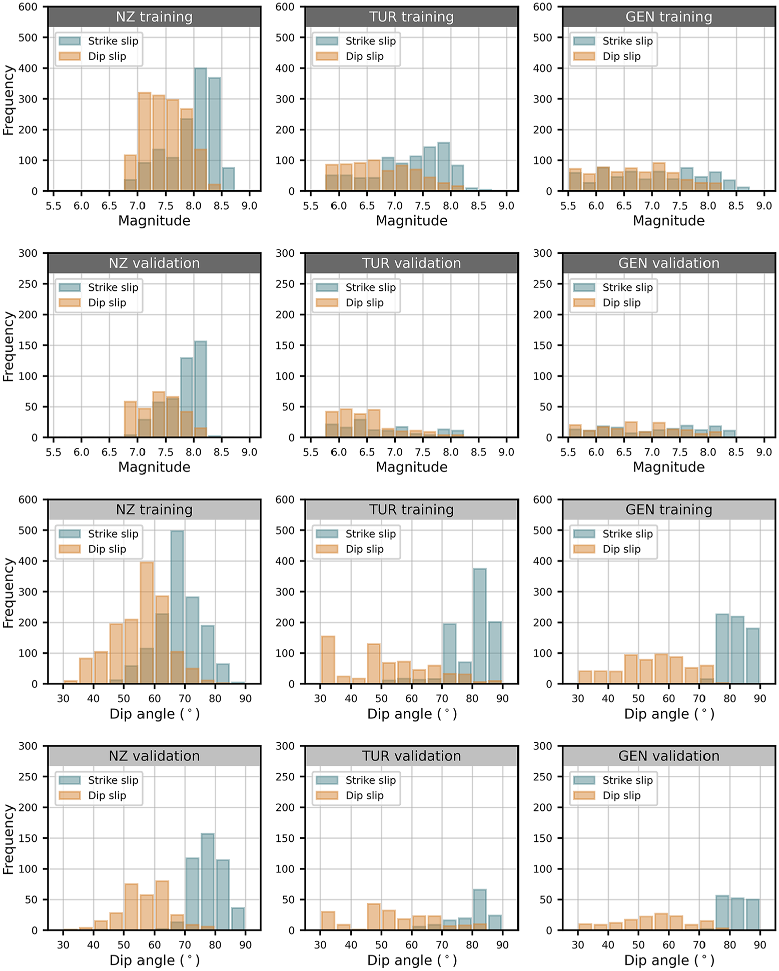
Distribution of the synthetic training and validation data sets with respect to magnitude, dip angle, and ERF. Lower bound magnitudes in NZ and TUR are determined by the fault models’ specific thresholds separating background from fault based seismicity. The lower bound magnitude of 5.5 for GEN was chosen to slightly extend our model’s applicability to lower magnitudes.

Deep learning–based modifier of moments implementation

The ability to grasp non-linear relations in data sets at great detail (e.g. Lecun et al., 2015), make deep learning an appealing candidate for the modeling of the complex, spatially variable patterns of moment modifiers. Classical deep learning, as implemented in this study, is a supervised machine learning method that dates back to the mid-twentieth century (McCulloch and Pitts, 1943; Rosenblatt, 1962; Rumelhart et al., 1986; Widrow and Hoff, 1960), where first attempts were made to design artificial neural networks, that is, model architectures that mimic the information processing workflows in the human brain (Bishop, 2006). One of deep learning’s most interesting key features is the fact that ANNs learn complex non-linear relations in data sets autonomously from the observation of pairs of predictive parameters and corresponding target parameters (in our case the representation of a rupture (predictive), and the corresponding moment modifiers (target)), such that the introduction of a priori knowledge via an inflexible, closed form equation becomes obsolete. However, due to the lack of a priori knowledge that could potentially constrain a model in case of data scarcity, a large set of data examples is required in order to train an ANN to the state where it can be utilized as a reliable predictive model. For a more thorough introduction to the field of deep learning we refer to the review of Lecun et al., (2015).

Deep learning has in recent years found various applications in seismology such as phase picking in seismic waveforms (Perol et al., 2018), fault detection in seismic images (Xiong et al., 2018), and ground motion modeling (Derras et al., 2014). Of particular interest is here the U-Net neural network architecture (Ronneberger et al., 2015), which operates on data in the shape of multi-channel images and is therefore a natural fit for the modeling of spatial data as demonstrated, for example, with the prediction of the strength of wireless communication signals in urban areas (Levie et al., 2020), or the prediction of spatially coherent maps of ground motion in the Kanto region (Lilienkamp et al., 2022). In this study, we employ the U-Net architecture to take the stack of maps describing an earthquake rupture $x_{i}$ as input, and provide estimates of the corresponding moment modifiers $y_{i}$ as output. Further details regarding the exact structure of the employed U-Net are given in the supplemental material S3.

After initialization, the U-Net neural network is merely a collection of random coefficients. As a consequence, if a model output ${\hat{y}}_{i}$ was generated from an input $x_{i}$ at this stage, it would simply be a random perturbation of the input, and not resemble the desired moment modifiers. Therefore, the model coefficients must be adjusted during a training procedure such that they produce a model output ${\hat{y}}_{i}$ similar to the desired moment modifiers $y_{i}$ . Technically, this is achieved via minimization of a normalized mean squared error ( $MS E^{*}$ ) loss function that quantifies the dissimilarity between the model output and the desired moment modifiers:

{MSE}_{i}^{*} (T) = \frac{1}{2 N_{p}} \sum_{k = 1}^{N_{p}} {[\frac{\bar{Δ μ_{dir, i, k}} (T) - \hat{\bar{Δ μ_{dir, i, k}}} (T)}{ϕ_{μ, i} (T)}]}^{2} + {[\frac{\bar{Δ σ_{dir, i, k}} (T) - \hat{\bar{Δ σ_{dir, i, k}}} (T)}{ϕ_{σ, i} (T)}]}^{2},

(4)

This is implemented using backpropagation (Rumelhart et al., 1986) and the Adam optimization algorithm (Kingma and Ba, 2015). We decided to normalize the loss function due to the strong period dependence of the directivity amplitude, such that equal attention is placed on all periods. Here, $N_{p} = 256 \times 256$ is the number of grid points on the map, $ϕ_{μ}$ is the standard deviation of all $\bar{Δ μ_{dir, k}}$ values and $ϕ_{σ}$ is the standard deviation of all $\bar{Δ σ_{dir, k}}$ values on the map. The update of model coefficients is not conducted for each training sample individually, but jointly for small subsets (mini batches) of training examples of various periods $T$ . The size of the minibatch is a model hyperparameter. A precise description of the training algorithm is provided in the supplemental material S3. During the training procedure, the U-Net iteratively learns to relate earthquake rupture descriptions $x_{i}$ from the training set to their corresponding moment modifiers $y_{i}$ . The U-Net is validated regularly with examples from the validation data set during training to ensure the models’ ability to generalize to previously unseen ruptures.

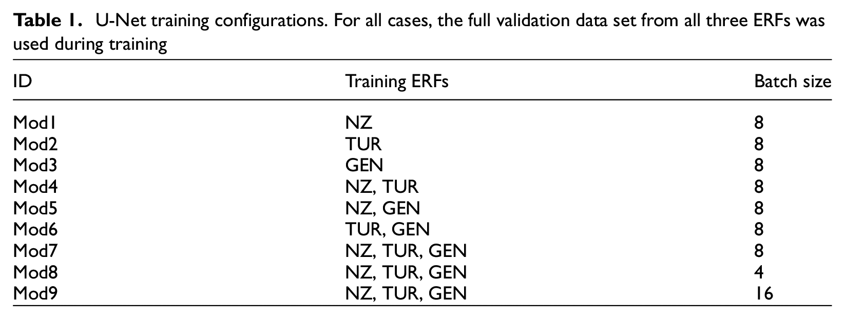
We tested nine different configurations of the training procedure, which are summarized in Table 1. We primarily varied the composition of the training data set in order to demonstrate the gain of using data from three different ERFs. For all configurations, we used the validation data set which is composed of ruptures from all three ERFs. For the configuration in which we use ruptures from all ERFs in the training set, we also tested the influence of the batch size hyperparameter.

Table 1.

U-Net training configurations. For all cases, the full validation data set from all three ERFs was used during training

ID	Training ERFs	Batch size
Mod1	NZ	8
Mod2	TUR	8
Mod3	GEN	8
Mod4	NZ, TUR	8
Mod5	NZ, GEN	8
Mod6	TUR, GEN	8
Mod7	NZ, TUR, GEN	8
Mod8	NZ, TUR, GEN	4
Mod9	NZ, TUR, GEN	16

Model performance evaluation

Initially, we evaluated the performance of the models across the nine configurations outlined in Table 1. For each model, we predicted moment modifiers for all samples in the validation data set and obtained the loss value w.r.t. the precalculated moment modifiers according to Equation 4. The cumulative distribution of loss values for each individual ERF is depicted in Figure 2. For the sake of clarity, we decided to present only the results obtained for a response period of $T$ = 3 s, however, additional periods are covered in the supplemental material S4 to this article. A primary finding was the notable disparity in performance when models trained with ruptures from one ERF were tested against ruptures from the other two ERFs (Figure 2a to c). Because the seismic properties in the training sets of the three ERFs are comparable (compare Figure 1), we attribute the significant performance variability among ruptures from different ERFs to the differences in geometrical complexity. Furthermore, the variable magnitude range among the ruptures in the three ERFs (compare Figure 1) might contribute to the variable generalization performance of the models in (a–c).

Figure 2.

Comparison of model performances on validation samples for configurations given in Table 1 and at a response period of $T$ = 3 s. The steep slope of the blue curve in (a) (Mod1) indicates a large amount of small loss values, and therefore good model performance, for NZ validation ruptures, whereas the shallow slope of the orange curve indicates a large amount of large loss values, and therefore poor generalization of Mod1 to the TUR data set. For comparison purposes, the performance of model Mod9 shown in (i) is also drawn in panels (a)–(h) as thick, transparent lines. $BS$ denotes the batch size.

Another significant observation is the considerable performance enhancement achieved by introducing a second ERF into the training set, evident in predicting ruptures from the third, still excluded ERF (Figure 2d to f). Notably, while this improvement is substantial in all cases, it is less pronounced for the most complex NZ ERF (compare Figure 2c and f). Comparing the performance gains resulting from the addition of a second ERF (e.g. Figure 2a and e) and the relatively smaller but still significant gains from using a third ERF (e.g. Figure 2e and i), led to the conclusion that training the U-Net model with ruptures from the three ERFs enables reasonable estimates of moment modifiers even for ruptures for previously unexplored ERFs. Although the influence of batch size was found to be mostly negligible, a slight advantage was observed with a batch size of 16 (model Mod9), hence further results shown in this study are obtained from this model.

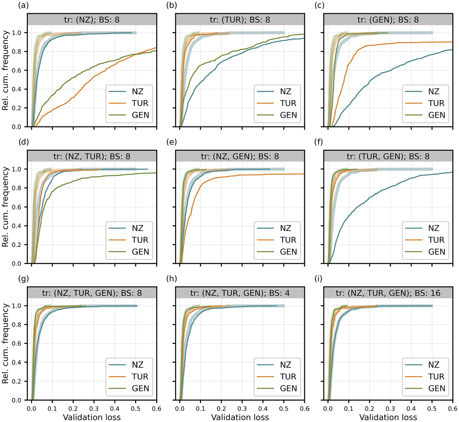
To illustrate the model’s predictive capabilities and its ability to handle challenging scenarios, we present three example predictions from model Mod9 in Figure 3. These examples were selected at the 99th, 90th, and 80th percentiles of obtained validation loss values in order to demonstrate that even in demanding cases, the model’s estimates of moment modifiers remain reasonably accurate. In the example from NZ (99th percentile), a clear shift in the strongest positive mean directivity adjustment from north to south is observed, alongside a smaller-than-targeted estimate of variability. Conversely, in the TUR example (90th percentile), differences in mean moment modifiers are less systematic, with only slight underestimation of variability. Finally, for the GEN example (80th percentile), only a minor systematic difference in the mean modifier is evident in the eastern region affected by positive amplification, with no systematic underestimation of variability observed upon visual inspection.

Figure 3.

Comparison of precalculated moment modifiers (d–f; j–l) with the U-Net reproductions (g–i; m–o) for the validation ruptures presented in a–c. The loss values of 0.244 (left column), 0.057 (center column), and 0.035 (right column) are representative for the 99th, 90th, and 80th percentile of obtained validation losses, respectively. Yellow lines in (b) and (c) indicate the top of rupture.

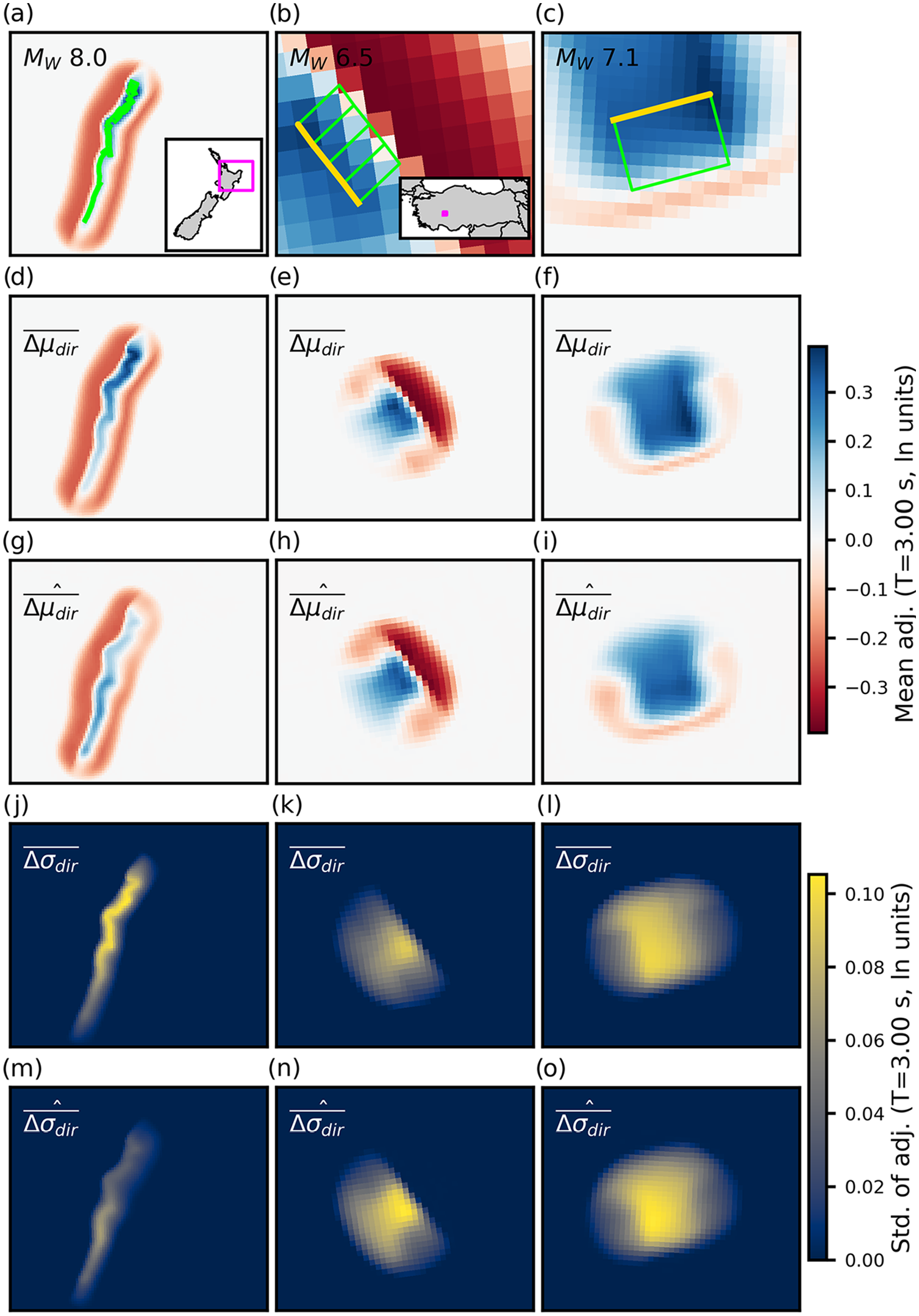
To offer a more comprehensive assessment of the overall model performance, we conducted a residual analysis, the results of which are presented in Figure 4. Residuals were calculated pixel-wise for validation ruptures for $1 \leq R_{rup} \leq 100$ km and $5.5 \leq M \leq 8$ . Across all depictions, the residuals appear largely centered around zero, albeit with some minor deviations.

Figure 4.

Distribution of pixel-wise model residuals from validation samples w.r.t. $R_{rup}$ and $M$ . Only sites with $1 \leq R_{rup} (km) \leq 100$ and $5.5 \leq M_{W} \leq 8$ are considered.

The standard deviation of the residuals for both moment modifiers consistently decrease with increasing $R_{r u p}$ (Figure 4a and c). This is expected, given that directivity primarily influences the near field. Similarly, standard deviations increase with magnitude (Figure 4b and d) reflecting the stronger directivity effects at larger magnitudes as per the model proposed by Bayless et al. (2020). From Figure 5 one can recognize a significant dependence of model uncertainty with increasing response period $T$ . This trend can be directly linked to the usage of a normalized loss function during training, which minimizes the relative misfit in order to put equal emphasis on all response periods. Arguably, the degree of misfit of the neural network moment modifier may be considered an additional source of variability that may, in certain circumstances, be relevant to consider within PSHA if the specific rupture and site configuration that leads to a larger misfit is pertinent for location of the target PSHA application. This may be identified through exploratory sensitivity analysis and could be partly mitigated by increasing the standard deviation in the moment modifier by reducing $Δ σ_{red}^{2}$ for the scenarios of critical importance.

Figure 5.

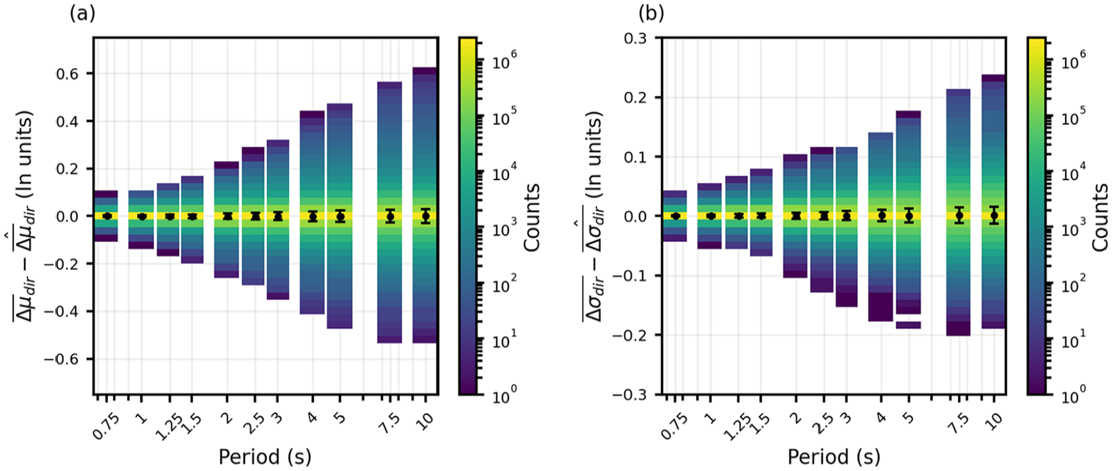
Distribution of pixel-wise model residuals from validation samples w.r.t. period $T$ . Only sites with $1 \leq R_{rup} (km) \leq 100$ and $5.5 \leq M_{W} \leq 8$ are considered.

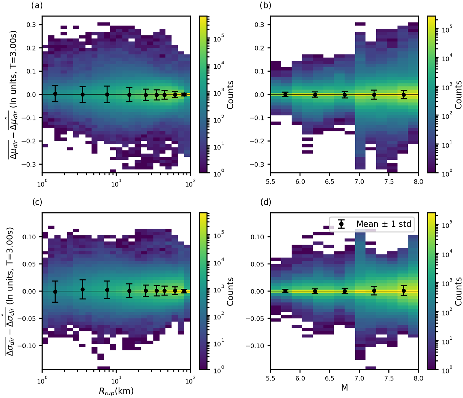
No discernible systematic trend with the dip angle of the rupture was identified. A detailed compilation of empirically determined biases and standard deviations depending on $T$ , $R_{rup}$ , and $M$ is provided in Tables S01-S11 in the supplementary material S5 accompanying this article.

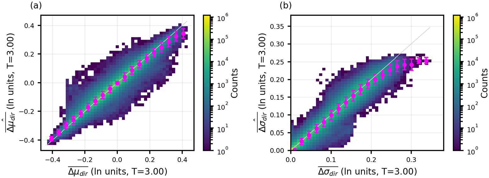
A direct comparison of pixel-wise, precomputed and estimated values of moment modifiers for validation samples at a period of $T = 3.0$ s is presented in Figure 6. While the model performs well in the ranges $- 0.4 \leq \bar{Δ μ_{dir}} \leq 0.2$ and $0 \leq \bar{Δ σ_{dir}} \leq 0.2$ , respectively, systematic underestimation of both moment modifiers must be stated for larger values. Especially the large, systematic underestimation of large values of $\bar{Δ σ_{dir}} \geq 0.25$ (Figure 6 b) requires some detailed analysis. We find that the most underestimated values at $\bar{Δ σ_{dir}} > 0.3$ belong to only three ruptures, one of which is presented as an exemplary case in Figure 7.

Figure 6.

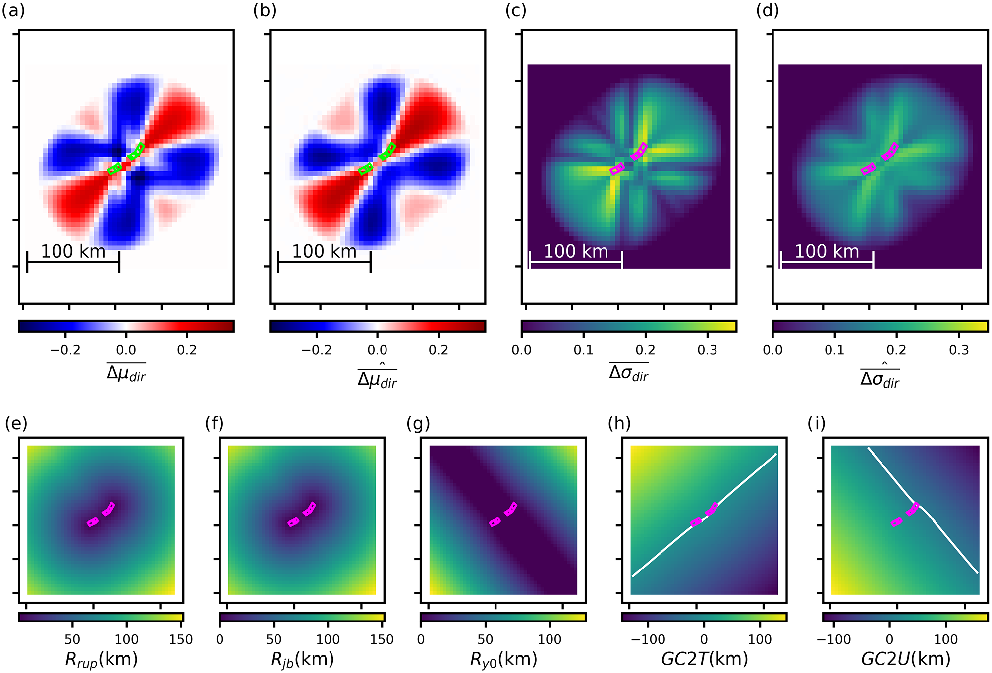
Pixelwise comparison of precalculated moment modifiers and model predictions for validation examples. Error bars indicate $\pm 1$ standard deviation. The straight line indicates the perfect fit.

Figure 7.

Example of a rupture from the NZ ERF (e–i) with exceptionally high values of $\bar{Δ σ_{dir}}$ at some pixels (c) that are significantly underestimated by the model (d). The mean moment modifier $\bar{Δ μ_{dir}}$ (a) and the corresponding model estimate (b) are in better agreement.

This $M = 6.93$ rupture from the NZ ERF is a relatively small rupture that, however, reveals the largest values of $\bar{Δ σ_{dir}}$ in the validation data set. We assume that this is the result of the offset between the two sub-ruptures and the chosen hypocenter distribution, which leads to a concentration of hypocenters toward the outer tips of the sub-ruptures. Therefore, compared to the case where the rupture had no step-over, sites close to the outer tips of the rupture experience fewer intermediate levels of amplification that would be caused by hypocenter locations in the center of the rupture. The remaining, more extreme, cases then lead to an increase in the variability $\bar{Δ σ_{dir}}$ . Although the roughly 10 km long step-over is hard to recognize visually from the representation of the rupture via the five distance metrics (Figure 7e to i), the pixel spacing of 5 km on the grid should theoretically enable the U-Net to reconstruct the rupture as indicated by the magenta colored outline. However, comparison of Figure 7a and b and c and d, respectively, creates the impression that the U-Net does not thoroughly grasp the finer nuances caused by the step-over and instead smoothes the patterns as if the gap did not exist. This is probably due to the fact that this specific case of a step-over together with the chosen hypocenter distribution leads to a very specific sample of hypocenter locations that is not representative for the average distribution in the training data set, and therefore the U-Net is not capable of thoroughly reproducing the resulting influence on the modifier patterns. In particular, since the hypocenter distribution is not given as an explicit model input, it is also not explicitly suggested that a rupture with a step-over should yield systematically different moment modifiers than contiguous ruptures. In this specific case, it is debatable whether such sharp, large amplitude features in the precalculated modifiers, which result from the theoretical description in the Bayless et al. (2020) model, would actually be observable in reality, or whether the more smoothed out appearance of the U-Net prediction might better explain real-world processes. However, since the objective of designing a surrogate model can only be to mimic as closely as possible the available synthetic data, such considerations should not find their way into future modeling attempts.

For the remaining two ruptures that generate comparably large exceptional values of $\bar{Δ σ_{dir}}$ , no drastic geometrical features such as step-overs are present. Again we suspect that an exceptional realization of hypocenter locations during the data generation might cause these exceptionally large values during data generation. In this regard, the more smoothed out appearance of the U-Net predictions are neither surprising nor particularly concerning, since such samples do then not represent the underlying distribution that the U-Net is supposed to grasp.

Implementation in PSHA

To demonstrate the application of the directivity model into probabilistic seismic hazard analysis, we consider the case of Turkey, and in particular the active fault sources contained within the recent 2020 European Seismic Hazard Model [ESHM20] (Basili et al., 2024; Danciu et al., 2024, 2021). A subset of this fault model formed part of the data set used to train the neural network, but in this case, we apply the resulting generalized directivity model to the complete set of ruptures generated by the fault source components of the model. The fault source model for ESHM20 is only one of the two source model logic tree branches used in the PSHA calculation, the other being a distributed seismicity (uniform area) source model. Furthermore, in the fault source model branches only earthquakes with $M_{W} \geq 6.5$ occur on the active faults themselves, while lower magnitude earthquakes are represented by a smoothed, gridded seismicity model (Danciu et al., 2024, 2021) to which directivity is not applied.

The Anatolian region provides a good case study for application for several reasons. First, the active fault source model contains faults with diverse styles of faulting, including long, fast-slipping strike-slip systems along the North and East Anatolian faults, extensional faulting in western Anatolia where the transform system gives way to backarc extension from the Hellenic subduction, and compressional faulting in eastern Turkey toward Lake Van and the Karliova Triple Junction. The geographical variation in style-of-faulting is shown in the upper map of Figure 8. 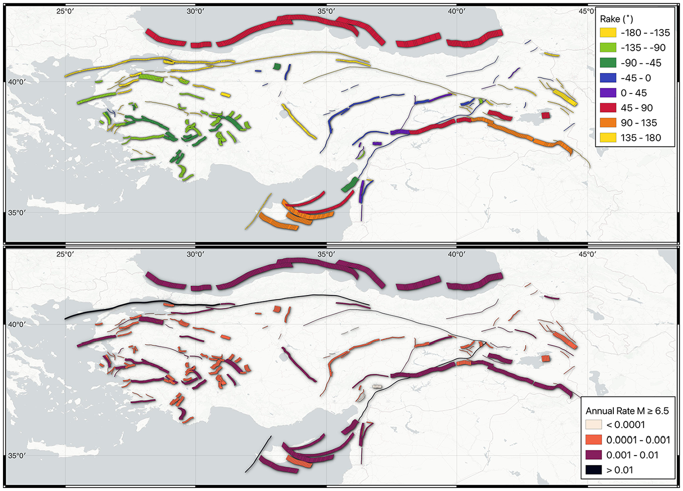Many of these fault systems are highly active, with rates of exceedance of $M_{W} 6.5$ on the order of more than 0.001 year⁻¹, and even as much as 0.01–0.03 years⁻¹ on the North and East Anatolian faults, which can be seen in the lower map of Figure 8. Earthquakes greater than $M_{W} 7.5$ have occurred in this region many times in the historical past, with the most recent being the 1999 Izmit earthquake ( $M_{W}$ 7.6) and two largest shocks of the 2023 Kahramanmaras earthquake sequence ( $M_{W} 7.8$ and $M_{W} 7.6$ ).

Figure 8.

Active fault sources for Turkey extracted from the 2020 European Seismic Hazard Model with color scaled according to rake $λ (^{°})$ (upper) and annual rate of occurrence of earthquakes with $M_{W} \geq 6.5$ .

In contrast to the ERF seismic hazard models developed for California and New Zealand using inversion (Field et al., 2014; Gerstenberger et al., 2022a), the ESHM20 adopts a floating rupture approach with earthquake recurrence described by a Gutenberg-Richter model truncated between a minimum and maximum magnitude. In this approach, each fault is described as a composite fault source with a fixed geometry and slip rate. Within the PSHA calculation, ruptures are generated for each magnitude considered within the magnitude frequency distribution using three-dimensional rupture surface whose area scales with earthquake size according to a specified magnitude frequency distribution, which in this case is Leonard (2014). If the rupture size is smaller than that of the entire composite fault source, the earthquake rupture forecast considers all the positions that the rupture can be placed uniformly within the fault surface given a specific stepping interval (5 km in this case). The rate of occurrence of that magnitude is split evenly between all of the possible corresponding ruptures can be distributed across the main fault surface. The composite fault sources represent model interpretations of the more complex geology, meaning that ruptures cannot contain offsets and/or step-overs but can change strike and, if necessary, dip along the rupture plane. This makes them more topologically simple than the inversion-based source ruptures seen in California and New Zealand. A total of 181 composite fault sources are considered in the model, covering Turkey, Cyprus and the Dead Sea transform. This results in 27,818 fault ruptures between $M_{W} 6.5$ and $M_{W} 8.5$ when assuming a floating rupture step distance of 5 km.

To assess the impact of directivity on the fault source PSHA for Turkey we run a complete probabilistic seismic hazard model for the highest weighted fault source branch of the model. For the ground motion model, ESHM20 adopts a scaled backbone logic tree, which considers the regionalized GMM of Kotha et al. (2020, 2022) as the backbone model and applies additional adjustments to describe epistemic uncertainty in source stress parameter and anelastic attenuation. For full details, see Weatherill et al. (2020) and Weatherill et al. (2024). As we are interested only in the relative change in seismic hazard given the inclusion of directivity for this illustrative application, we consider only the core backbone GMM, which is regionalized for application to Turkey, but do not consider all the possible branches of the scaled backbone logic tree. As the moment modifier model is based upon the directivity amplification model of Bayless et al. (2020), their corresponding reduction factors for the within-event variability of the ground motion model are implemented in this calculation to determine $Δ σ_{red} (T)$ , as per Equation 3.

The seismic hazard terms of the 3-s spectral acceleration, $Sa (3.0 s)$ with a 10% probability of being exceeded in 50 years is shown in Figure 9. Here the change in seismic hazard from incorporating directivity using the generalized neural network modifier of moments model can be seen in the difference map. The most obvious feature is a clear increase in hazard on the order of 25%–30% along main North and East Anatolian Fault systems. This reflects the density of rupture locations and the high activity rates of the two principal faults in the Anatolian region. Elsewhere the change in hazard is more variable, with moderate increases in seismic hazard on the order of 10%–15% on the up-dip sides of the more active reverse faults in eastern Turkey and the Caucasus as well as in the extensional faults in southwestern Turkey. These are accompanied by net decreases in hazard on the down-dip sides of the faults.

Figure 9.

$Sa (3.0 s)$ with a 10 % probability of exceedance in 50 years without directivity (top), with directivity (middle) and percent change in the seismic hazard from including directivity (bottom). These results are specific to the Bayless et al. (2020) directivity model, the assumed hypocenter distributions, and equal probability of 0.5 for unilateral and bilateral rupture propagation for strike-slip ruptures. Changing any of these assumptions may have substantial impact on the resulting change in seismic hazard.

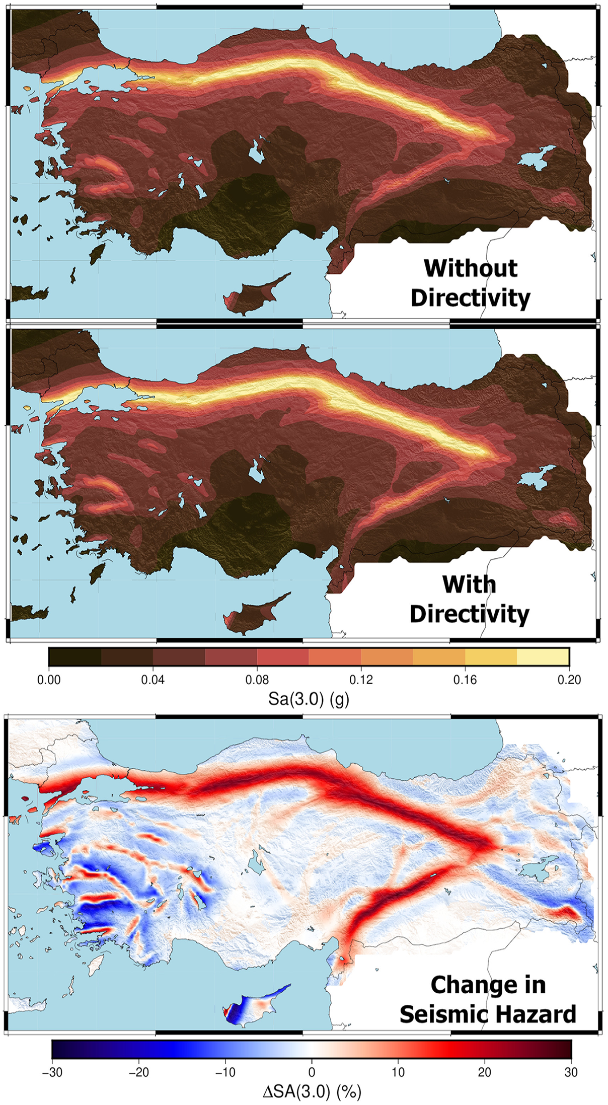
Stronger polarization of the changes in hazard are seen in the extensional regions of western Turkey rather than around the compressional faults in eastern Turkey, which seems at first counter-intuitive given that we would likely expect higher directivity amplification on reverse faults, as suggested by dynamic rupture simulations on dipping faults (Oglesby et al., 2000). This pattern in the change in seismic hazard is controlled by higher activity rate and density of faults in western Turkey and the fact that the underlying Bayless et al. (2020) directivity model on which the modifier of moments model is calibrated only distinguishes between strike-slip and dip-slip faults, and not between reverse and normal faults. As the NGA West 2 data set upon which the Bayless et al. (2020) model was fit contains a much greater proportion of reverse faulting ruptures than normal faulting, the patterns of amplification with respect to the up- and down-dip projections of the rupture in the moment modifier models will reflect more the reverse faulting case. The relevant point here is that the changes in seismic hazard around the extensional faults in western Turkey may be larger than we had expected given style of faulting, and may not necessarily be present to the same extent were one to use a directivity amplification model that distinguishes between reverse and normal dip-slip faults.

The example applications demonstrated that the neural network modifier of moments model can be applied to realistic fault-based seismic hazard models. The amplitude of the change in seismic hazard is, of course, dependent on spectral period, with peak changes on the order of ±3%–5% for $Sa (1.0 s)$ to as much as 50% at very long periods ( $T \geq 5 s$ ). For Istanbul in particular, however, the expected increase in hazard is on the order of 2.5% for $Sa (1.0 s)$ , 15.5% for $Sa (3.0 s)$ and 21% for $Sa (5.0 s)$ . It should of course be re-iterated that the exact degree of amplification or de-amplification is dependent not only on the period of vibration being considered but also to this specific combination of the Bayless et al. (2020) directivity amplification model and the hypocentre distribution assumed within the moment modifier approach. Alternative models will inevitably yield different results than those shown here, some potentially reducing the net influence of directivity on the seismic hazard.

Although execution of the neural network modifier of moments model did increase the computational time of the calculation compared to the execution of the PSHA without directivity, the total running time was not prohibitive and remained considerably smaller than that of running a fully randomized hypocenter approach with this same underlying directivity model. The increased computational effort emerged from the need to calculate the distances measured required by the U-Net at the U-Net reference grid sites in addition to those required by the selected GMM at the hazard calculation target sites, and then from interpolating the moment modifiers from the U-Net reference grid to the target sites. The exact increase in calculation time and computational resources will likely vary from one software to another, and potentially from one calculation configuration to another, depending on the efficiency of the implementation of these additional steps. It should also be noted that other directivity models such as Chiou and Youngs (2014) and Bayless et al. (2024) require racetrack centering in forward application, a process that increases computational costs for application of directivity in PSHA at scale. In light of this, the computational benefit to cost ratio of using neural network based moment modifier models will likely increase when using other directivity models that require racetrack centering.

Discussion

In the “Model performance evaluation” section, we identified few ruptures for which certain combinations of the chosen hypocenter distributions, the sampled hypocenter locations, and the rupture geometries lead to exceptionally large values of the precalculated $\bar{Δ σ_{dir}}$ , that could not be reproduced by the U-Net model. Since the number of hypocenters that are sampled per rupture during data generation is finite ( $N_{SAMP}$ = 250), and the synthetic data set consists of over 5000 ruptures, it is expected that few individual ruptures end up with an unusual sample of hypocenter locations that may not appear at first to represent the underlying distribution. Since the precalculated moment modifiers do not exactly represent the average directivity effect, it is of little surprise and not particularly worrying that the U-Net predictions differ substantially from the targets.

This perspective fundamentally differs from the overfitting approach presented in (Weatherill and Lilienkamp, 2023), where the ANN model was forced to adapt as closely as possible to every individual precalculated moment modifier for every rupture. Ultimately, it is the decision of the modeler to assess to which degree the underlying dataset is to be trusted versus how much emphasis is put on maximizing the ability to generalize to novel ruptures at the cost of missing some of the finer, though potentially artificial, details in the synthetic data set.

Considering the initial purpose of the model developed in this study as a globally applicable model, we focus on the fact that even if the U-Net encounters ruptures with unfamiliar geometrical features, which is very likely to happen when applied to ruptures outside the ERFs considered in this study, it is still capable of providing amplification patterns that agree on the large scale very well with the manually calculated moment modifiers, and that the discrepancies are only revealed in the finer nuances. This property might lead to distorted estimates of the seismic hazard at few sites that are located in the small affected areas, and the hazard of which is largely dominated by this one particular rupture.

We consider our model Mod9 to be applicable to ruptures from the NZ and TUR ERFs, as well as simple planar ruptures with the following ranges of magnitudes and dip angles $ϕ$ :

$5.75 \leq M \leq 8.0$

$30 \leq ϕ \leq 90$ for dip-slip ruptures

$45 \leq ϕ \leq 90$ for strike-slip ruptures

$R_{rup} \leq 1217$ km

$R_{jb} \leq 1219$ km

$R_{y 0} \leq 1147$ km

-1050 km $\leq GC 2_{t} \leq 1, 212$ km

-1094 km $\leq GC 2_{u} \leq 1, 683$ km

Although the magnitude range in our training set is actually larger than the one suggested here, we emphasize that $5.5 \leq M \leq 5.75$ only occur for the GEN ruptures, such that the model may not properly generalize to geometrically more complex cases at this magnitude range. Furthermore, although $M > 8.0$ is considered during model training, the upper limit of applicability is suggested by Bayless et al. (2020) to be $M_{W}$ 8.0. When applied to ruptures outside the ERFs utilized in this study, users should verify that the geometrical properties are somewhat comparable to the ones presented in this study, that is, ruptures should consist of planar segments and the level of complexity, that is, number of step-overs and branches within a rupture, should not be larger than for those ruptures in the training set. To give an impression of the level of complexity our model can handle, we provide additional examples in the supplemental material S6.

The grid spacing of 5 km for both the predictive parameters and the moment modifiers was chosen to achieve a good compromise between demonstrating the capability of our model to grasp the spatial patterns of the moment modifiers and limiting the computational effort of generating the synthetic data set and training the ANN model. We note that if the number and variety of earthquake ruptures in the synthetic data set is too small, this rather coarse resolution might pose a certain limitation in resolving the spatial moment modifier patterns in the very near field, especially for small magnitude ruptures. The question of whether the resolution of the grid spacing in the U-Net has a significant impact on the uncertainty of the moment modifiers is a relevant one for seismic hazard analysis. We attempt to quantify this in an experiment comparing the calculated moment modifiers for a subset of ruptures on a higher resolution (2 km × 2 km) grid with the predicted moment modifiers from the original 5 km × 5 km U-Net interpolated to the finer grid (as would be the means of implementation in a PSHA software). The details of the experiment and the results are shown in supplemental material S7, but the key finding is that the additional error that comes from using the coarser grid U-Net to predict the finer scale distributions was on the order of around 0.0003 natural log units. While we do not discount the possibility that there may be specific source and site configurations under which the resolution mat be more relevant, for the majority of cases we do not expect this error to have a significant impact on the seismic hazard calculations.

Several assumptions were made during the preparation of the synthetic data set that should be kept in mind when applying the model in practice. Most notably, the model predictions are highly influenced by the choice of the Bayless et al. (2020) directivity model, the fixed number of considered hypocenters per rupture, the assumed distributions of hypocenter locations and, as a consequence, the assumption of equal probability for bilateral and unilateral rupture propagation for strike-slip ruptures. We consider these assumptions reasonable for the development a globally applicable average model, however, we also note that on regional scale, more skewed distributions might better represent the regional characteristics where a preference for a particular rupture direction may be identified. For example, both theoretical considerations (Shi and Ben-Zion, 2006) and empirical evidence (Türker et al., 2022) hint toward preferred directions of rupture propagation along the North Anatolian fault zone close to Istanbul, which contradicts the previously mentioned assumptions. Moreover, a constant density of hypocenters along earthquake ruptures might be a worthwhile option to explore contrary to a fixed number of hypocenters per rupture. The specific form of such an alternative hypocenter distribution and the manner in which it would be calibrated given the available seismological data for a region remain an open question for the engineering seismological community to answer. We emphasize at this point that changing any of the assumptions mentioned above, requires the generation of an entirely new data set and the training of a new neural network. Considering the application of neural network based modifier of moments models in PSHA, where directivity is deemed important for the application in question we suggest to introduce additional branches into existing backbone models, such that both the consideration of directivity effects as such, but also the epistemic uncertainty of the underlying assumptions can be incorporated properly in the seismic hazard.

Summary and conclusions

In this study, we have developed a neural network–based model that takes as input the representation of an earthquake rupture and provides as output maps of modifiers for the moments of the ground motion distribution predicted by a ground motion model to account for directivity effects in the vicinity of the rupture. For training, we used a synthetic data set incorporating ruptures and corresponding precalculated moment modifiers from three different source models. The model operates on fixed sized areas of 1280 km × 1280 km at a cell size of (5 km)². We find that the model yields good estimates of moment modifiers not only for simple planar ruptures, but also for more complex, branching ruptures with step-overs. Among several assumptions, the choice of symmetric hypocenter distributions and the choice of using the Bayless et al. (2020) directivity model for the generation of the synthetic data set has a direct influence on the predicted moment modifiers, which should be considered when applying the model in practice. From the validation of the model with earthquake ruptures that were not used during training we noticed a moderate variability of model performance, especially in explaining small scale details, that can be partially related to imperfections in the underlying synthetic data set. From the small number of affected ruptures, and the still reasonable model predictions on the large scale we conclude, however, that this variability does not critically affect the results of seismic hazard computations utilizing our model. Therefore we consider our model applicable to earthquake ruptures in PSHA, scenario hazard and risk analysis and possibly other applications on a global scale, as long as the seismic properties and the geometric complexity are comparable to those in the used training set. To confirm this finding, we successfully applied our model in a PSHA calculation for Turkey, using an experimental branch of the OpenQuake software. Considerable changes in the seismic hazard at the 475-year return period for $SA (3.0 s)$ of up to $\pm 30 %$ highlight the importance of incorporating directivity in future PSHA studies. Although the computational effort of explicitly incorporating directivity effects with our model is increased, the suggested approach is significantly more efficient compared to the straightforward full hypocenter randomization approach. As a consequence, our model enables a practical option to explicitly incorporate directivity effects in regional-scale PSHA studies with advanced source models in the future.

Supplemental Material

sj-pdf-1-eqs-10.1177_87552930251340668 – Supplemental material for Efficient incorporation of rupture directivity into probabilistic seismic hazard analysis using a deep learning–based approach

Supplemental material, sj-pdf-1-eqs-10.1177_87552930251340668 for Efficient incorporation of rupture directivity into probabilistic seismic hazard analysis using a deep learning–based approach by Henning Lilienkamp and Graeme Weatherill in Earthquake Spectra

Footnotes

Acknowledgements

The authors want to thank Jeff Bayless, Kyle Withers, Brian Chiou, Brian Kelly, and Paul Somerville for stimulating discussions, reviews, and valuable feedback on the research. In addition, the authors want to thank Fabrice Cotton for feedback and review of the original manuscript. This work utilized high-performance computing resources made possible by funding from the Ministry of Science, Research and Culture of the State of Brandenburg (MWFK) and are operated by the IT Services and Operations unit of the Helmholtz Centre Potsdam. Chat-GPT v.4o (/) was used to rephrase some paragraphs to make them more easily accessible to the audience.

Declaration of conflicting interests

The author(s) declared no potential conflicts of interest with respect to the research, authorship, and/or publication of this article.

Funding

The author(s) disclosed receipt of the following financial support for the research, authorship, and/or publication of this article: We acknowledge support by the European Union’s Horizon 2020 Research and Innovation Programme (DT-GEO Grant 101058129).

ORCID iDs

Henning Lilienkamp

Graeme Weatherill

Data and resources

Computation of the seismic hazard is undertaken using a customized version of OpenQuake (Pagani et al., 2014). The OpenQuake-compatible implementation of the Bayless et al. (2020) directivity model was verified and tested against code provided by the authors available at https://www.jeff-bayless.com/papers/. Maps shown in this article were constructed using QGIS available at https://qgis.org, Generic Mapping Tools (GMT v.6) available at https://www.generic-mapping-tools.org/, and Basemap (v.1.4.1) available at https://matplotlib.org/basemap/stable/. Topography and bathymetry shown in the maps is taken from the 2023 Gridded Bathymetric Dataset produced by the General Bathymetric Chart of the Oceans (GEBCO Bathymetric Compilation Group, 2023). Neural network training, inference, and optimization was implemented with Tensorflow (Abadi et al., 2015), whereas all other data analyses utilized the multiple tools from the Scientific Python ecosystem (Numpy, Scipy, Pandas, GeoPandas, Matplotlib, etc.) available at https://numfocus.org/. Some figures were designed with Inkscape available at https://inkscape.org/de/. The seismic source models utilized in this study are available via http://hazard.efehr.org/en/Documentation/specific-hazard-models/europe/eshm2020-overview/eshm20-seismogenic-sources/ (European Seismic Hazard Model 2020) and https://www.gns.cri.nz/research-projects/new-zealand-community-fault-model/ (New Zealand Community Fault Model). All websites were accessed last on 24 June 2024. The python codes developed within the scope of this study are available via Zenodo: https://doi.org/10.5281/zenodo.15118499. The final calibrated model from this study (model Mod9) is available for usage via pypi: /. The supplemental material to this article contains: S1—A figure and text illustrating the generation of moment modifiers, S2—Figures and text describing the training/validation data split using multidimensional scaling. S3—Text, figures, and tables with details regarding the U-Net architecture and training procedure. S4—The same figures presented in section “Model performance evaluation” for additional response periods. S5—Tables describing the model uncertainties obtained from misfits on validation samples. S6—A random selection of pairs of precalculated and reproduced moment modifiers from the validation data set. S7—Exploration of U-Net resolution uncertainty and impact. The synthetic data set utilized for training our model is reproducible with the information given in this manuscript. Due to its enormous size, the authors decided not to host it on a public repository. If needed, the authors are happy to provide additional information on the data generation workflow.

Supplemental material

Supplemental material for this article is available online.

References

Abadi

Agarwal

Barham

Brevdo

Chen

Citro

Corrado

Davis

Dean

Devin

Ghemawat

Goodfellow

Harp

Irving

Isard

Jozefowicz

Jia

Kaiser

Kudlur

Levenberg

Mané

Schuster

Monga

Moore

Murray

Olah

Shlens

Steiner

Sutskever

Talwar

Tucker

Vanhoucke

Vasudevan

Viégas

Vinyals

Warden

Wattenberg

Wicke

Zheng

(2015) TensorFlow: Large-scale machine learning on heterogeneous systems. Technical Report. Available at: https://zenodo.org/record/6574269. Accessed 24 June 2024.

Abrahamson

(2000) Effects of rupture directivity on probabilistic seismic hazard analysis. In: Proceedings of the Sixth international conference on seismic zonation: Managing earthquake risk in the 21st century, Palm Springs, CA, 12–15 November.

Al Atik

Gregor

Mazzoni

Bozorgnia

(2023) Directivity-based probabilistic seismic hazard analysis for the state of California: Report 2, Directivity Implementation. Technical Report, University of California, Los Angeles, Los Angeles, CA, May.

Basili

Danciu

Beauval

Sesetyan

Vilanova

Adamia

Arroucau

Atanackov

Baize

Canora

Caputo

Carafa

MMC

Cushing

Custódio

Demircioglu Tumsa

Duarte

Ganas

García-Mayordomo

Gómez de la Peña

Gràcia

Jamšek Rupnik

Jomard

Kastelic

Maesano

Martín-Banda

Martínez-Loriente

Neres

Perea

Šket Motnikar

Tiberti

Tsereteli

Tsironi

Vallone

Vanneste

Zupančič

Giardini

(2024) The European fault-source model 2020 (EFSM20): Geologic input data for the European seismic hazard model 2020. Natural Hazards and Earth System Sciences 24: 3945–3976.

Bayless

Abrahamson

Norman Somerville

(2024) A rupture directivity adjustment model and its application in seismic hazard. Earthquake Spectra 41: 753–781.

Bayless

Somerville

Skarlatoudis

(2020) A rupture directivity adjustment model applicable to the NGA-West2 ground motion models and complex fault geometries. Technical Report, U.S. Geological Survey Technical Report, Reston, VA, April.

Bertero

Mahin

Herrera

(1978) Aseismic design implications of near-fault San Fernando earthquake records. Earthquake Engineering & Structural Dynamics 6(1): 31–42.

Bishop

(2006) Pattern Recognition and Machine Learning. New York: Springer, pp.978–971.

Bradley

Quigley

Van Dissen

Litchfield

(2014) Ground motion and seismic source aspects of the Canterbury earthquake sequence. Earthquake Spectra 30(1): 1–15.

10.

Chiou

Youngs

(2014) Update of the Chiou and Youngs NGA model for the average horizontal component of peak ground motion and response spectra. Earthquake Spectra 30(3): 1117–1153.

11.

Cornell

(1968) Engineering seismic risk analysis. Bulletin of the Seismological Society of America 58(5): 1583–1606.

12.

Danciu

Giardini

Weatherill

Basili

Nandan

Rovida

Beauval

Bard

Pagani

Reyes

Sesetyan

Vilanova

Cotton

Wiemer

(2024) The 2020 European seismic hazard model: Overview and results. Natural Hazard and Earth System Sciences 2024: 1–36.

13.

Danciu

Nandan

Reyes

Basili

Weatherill

Beauval

Rovida

Vilanova

Sesetyan

Bard

Cotton

FSW

Giardini

(2021) The 2020 update of the European Seismic Hazard Model—ESHM20: Model Overview. Technical Report 001, V1.0.0, European Facility for Earthquake Hazard and Risk (EFEHR), Zurich, August.

14.

Derras

Bard

Cotton

(2014) Towards fully data driven ground-motion prediction models for Europe. Bulletin of Earthquake Engineering 12(1): 495–516.

15.

Donahue

Stewart

Gregor

Bozorgnia

(2019) Ground-motion directivity modeling for seismic hazard applications. Technical Report PEER Report No. 2019/03, Pacific Earthquake Engineering Research Center (PEER), Berkeley, CA, January.

16.

Field

Arrowsmith

Biasi

Bird

Dawson

Felzer

Jackson

Johnson

Jordan

Madden

Michael

Milner

Page

Parsons

Powers

Shaw

Thatcher

Weldon

Zeng

(2014) Uniform California Earthquake Rupture Forecast, version 3 (UCERF3)-The time-independent model. Bulletin of the Seismological Society of America 104(3): 1122–1180.

17.

Gerstenberger

Bora

Bradley

DiCaprio

Van Dissen

Atkinson

Chamberlain

Christophersen

Clark

Coffey

(2022a) New Zealand National Seismic Hazard Model 2022 Revision: Model, hazard and process overview. Technical Report GNS Science Report 2022/57, GNS Science, Lower Hutt, September.

18.

Gerstenberger

Van Dissen

Rollins

DiCaprio

Chamberlain

Christophersen

Coffey

Ellis

Iturrieta

Johnson

Litchfield

Rastin

Seebeck

Stirling

Thingbaijam

(2022b) The seismicity rate model for the 2022 New Zealand National Seismic Hazard Model. Technical Report GNS Science Report 2022/47, GNS Science, Lower Hutt, January.

19.

Hall

Heaton

Halling

Wald

(1995) Near-source ground motion and its effects on flexible buildings. Earthquake Spectra 11(4): 569–605.

20.

Kelly

Withers

Moschetti

(2022) Development of a seismic directivity adjustment model to the median and aleatory variability of ground motion models. In: AGU Fall Meeting, Chicago, I, 12–16 December, pp.12–16.

21.

Kingma

(2015) Adam: A method for stochastic optimization. In: 3rd International Conference on Learning Representations, ICLR—Conference Track Proceedings, San Diego, CA, 7–9 May.

22.

Kotha

Weatherill

Bindi

Cotton

(2020) A regionally-adaptable ground-motion model for shallow crustal earthquakes in Europe. Bulletin of Earthquake Engineering 18: 4091–4125.

23.

Kotha

Weatherill

Bindi

Cotton

(2022) Near-source magnitude scaling of spectral accelerations: Analysis and update of Kotha et al. (2020) model. Bulletin of Earthquake Engineering 20: 1343–1370.

24.

Lecun

Bengio

Hinton

(2015) Deep learning. Nature 521(7553): 436–444.

25.

Leonard

(2014) Self-consistent earthquake fault scaling relations: Update and extension to stable continental strike-slip faults. Bulletin of the Seismological Society of America 104: 2953–2965.

26.

Levie

Yapar

Kutyniok

Caire

(2020) Pathloss prediction using deep learning with applications to cellular optimization and efficient D2D link scheduling. In: ICASSP, IEEE International Conference on Acoustics, Speech and Signal Processing—Proceedings, Barcelona, 4–8 May, pp.8678–8682. New York: IEEE.

27.

Lilienkamp

von Specht

Weatherill

Caire

Cotton

(2022) Ground-motion modeling as an image processing task: Introducing a neural network based, fully data-driven, and nonergodic approach. Bulletin of the Seismological Society of America 112(3): 1565–1582.

28.

McCulloch

Pitts

(1943) A logical calculus of the ideas immanent in nervous activity. The Bulletin of Mathematical Biophysics 5(4): 115–133.

29.

Mai

Aspiotis

Aquib

Cano

Castro-Cruz

Espindola-Carmona

Liu

Matrau

Nobile

Palgunadi

Ribot

Parisi

Suhendi

Tang

Yalcin

Avşar

Klinger

Jónsson

(2023) The destructive earthquake doublet of 6 February 2023 in South-Central Türkiye and Northwestern Syria: Initial observations and analyses. The Seismic Record 3(2): 105–115.

30.

Mavroeidis

Dong

Papageorgiou

(2004) Near-fault ground motions, and the response of elastic and inelastic single-degree-of-freedom (SDOF) systems. Earthquake Engineering and Structural Dynamics 33(9): 1023–1049.

31.

Melgar

Hayes

(2019) The correlation lengths and hypocentral positions of great earthquakes. Bulletin of the Seismological Society of America 109(6): 2582–2593.

32.

Miller

Rice

(1983) Discrete approximations of probability distributions. Management Science 29(3): 352–362.

33.

Oglesby

Archuleta

Nielsen

(2000) The three-dimensional dynamics of dipping faults. Bulletin of the Seismological Society of America 90(3): 616–628.

34.

Pagani

Monelli

Weatherill

Danciu

Crowley

Silva

Henshaw

Butler

Nastasi

Panzeri

Simionato

Vigano

(2014) Openquake engine: An open hazard (and risk) software for the global earthquake model. Seismological Research Letters 85(3): 692–702.

35.

Page

Field

Milner

Powers

(2014) The UCERF3 grand inversion: Solving for the long-term rate of ruptures in a fault system. Bulletin of the Seismological Society of America 104(3): 1181–1204.

36.

Perol

Gharbi

Denolle

(2018) Convolutional neural network for earthquake detection and location. Science Advances 4(2): 2–10.

37.

Ronneberger

Fischer

Brox

(2015) U-net: Convolutional networks for biomedical image segmentation. Lecture Notes in Computer Science 9351: 234–241.

38.

Rosenblatt

(1962) Principles of Neurodynamics: Perceptrons and the Theory of Brain Mechanisms. Vol. 55. Washington, DC: Spartan Books.

39.

Rumelhart

Hinton

Williams

(1986) Learning Representations by Back-Propagating Errors. Nature 323(9): 533–536.

40.

Seebeck

Van Dissen

Litchfield

Barnes

Nicol

Langridge

Barrell

Villamor

Ellis

Rattenbury

Bannister

Gerstenberger

Ghisetti

Sutherland

Hirschberg

Fraser

Nodder

Stirling

Humphrey

Bland

Howell

Mountjoy

Moon

Stahl

Spinardi

Townsend

Clark

Hamling

Cox

de Lange

Wopereis

Johnston

Morgenstern

Coffey

Eccles

Little

Fry

Griffin

Townend

Mortimer

Alcaraz

Massiot

Rowland

Muirhead

Upton

Lee

(2023) The New Zealand Community Fault Model–version 1.0: An improved geological foundation for seismic hazard modelling. New Zealand Journal of Geology and Geophysics 67: 209–229.

41.

Shi

Ben-Zion

(2006) Dynamic rupture on a bimaterial interface governed by slip-weakening friction. Geophysical Journal International 165(2): 469–484.

42.

Somerville

(2003) Magnitude scaling of the near fault rupture directivity pulse. Physics of the Earth and Planetary Interiors 137(1–4): 201–212.

43.

Somerville

Smith

Graves

Abrahamson

(1997) Modification of empirical strong ground motion attenuation relations to include the amplitude and duration effects of rupture directivity. Seismological Research Letters 68(1): 199–222.

44.

Spudich

Chiou

(2015) Strike-parallel and strike-normal coordinate system around geometrically complicated rupture traces— Use by NGA-West2 and Further Improvements. Technical Report, United States Geological Survey, Reston, VI, March.

45.

Spudich

Bayless

Baker

Chiou

Rowshandel

Shahi

Somerville

(2013) Final report of the NGA-West2 directivity working group. Technical Report, PEER Report No. 2013/09, Pacific Earthquake Engineering Research Center (PEER), Berkeley, CA, September.

46.

Stirling

McVerry

Gerstenberger

Litchfield

Van Dissen

Berryman

Barnes

Wallace

Villamor

Langridge

Lamarche

Nodder

Reyners

Bradley

Rhoades

Smith

Nicol

Pettinga

Clark

Jacobs

(2012) National seismic hazard model for New Zealand: 2010 update. Bulletin of the Seismological Society of America 102(4): 1514–1542.

47.

Türker

Cotton

Pilz

Weatherill

(2022) Analysis of the 2019 Mw 5.8 Silivri earthquake ground motions: Evidence of systematic Azimuthal variations associated with directivity effects. Seismological Research Letters 93(2A): 693–705.

48.

Van Dissen

Seebeck

Wallace

Rollins

Gerstenberger

Howell

DiCaprio

Williams

(2022) New Zealand national seismic hazard model 2022: Geologic and subduction interface deformation models. Technical Report GNS Science Report 2022/31, GNS Science, Lower Hutt, November.

49.

Wald

Heaton

(1994) Spatial and temporal distribution of slip for the 1992 Landers, California, earthquake. Bulletin—Seismological Society of America 84(3): 668–691.

50.

Watson-Lamprey

(2018) Capturing directivity effects in the mean and aleatory variability of the NGA-West2 ground-motion prediction equations. Technical Report 2018-04, Pacific Earthquake Engineering Research Center (PEER), Berkeley, CA, November.

51.

Weatherill

Lilienkamp

(2023) Capturing directivity in probabilistic seismic hazard analysis for New Zealand: Challenges, implications, and a machine learning approach for implementation. Bulletin of the Seismological Society of America 114(1): 373–398.

52.

Weatherill

Kotha

Cotton

(2020) A regionally-adaptable “scaled backbone” ground motion logic tree for shallow seismicity in Europe: Application to the 2020 European seismic hazard model. Bulletin of Earthquake Engineering 18: 5087–5117.

53.

Weatherill

Kotha

Danciu

Vilanova

Cotton

(2024) Modelling seismic ground motion and its uncertainty in different tectonic contexts: Challenges and application to the 2020 European seismic hazard model (eshm20). Natural Hazards and Earth System Sciences 24(5): 1795–1834.

54.

Widrow

Hoff

(1960) Adaptive switching circuits. In: Widrow

Hoff

(eds) IRE WESCON Convention Record, Vol. 4. Cambridge, MA: The MIT Press, pp.96–104.

55.

Withers

Kelley

Bayless

Moschetti

Powers

(2024a) Methods to evaluate and improve the modelling of rupture directivity in assessment of seismic hazard. In: Proceedings of the 18th world conference on earthquake engineering, Milan, Italy, 30 June–5 July.

56.

Withers

Moschetti

Powers

Petersen

Graves

Aagaard

Baltay

Luco

Wirth

Rezaeian

Thompson

(2024b) Integration of rupture directivity models for the US National Seismic Hazard Model. Earthquake Spectra 40(2): 1066–1098.

57.

Xie

(2019) Strong-motion directionality and evidence of rupture directivity effects during the chi-chi Mw 7.6 earthquake. Bulletin of the Seismological Society of America 109(6): 2367–2383.

58.

Xiong

Wang

Benhassan

Ali

Luo

(2018) Seismic fault detection with convolutional neural network. Geophysics 83(5): O97–O103.

Supplementary Material

Please find the following supplemental material available below.

For Open Access articles published under a Creative Commons License, all supplemental material carries the same license as the article it is associated with.

For non-Open Access articles published, all supplemental material carries a non-exclusive license, and permission requests for re-use of supplemental material or any part of supplemental material shall be sent directly to the copyright owner as specified in the copyright notice associated with the article.

0.00 MB

13.18 MB