Direct quality prediction in resistance spot welding process: Sensitivity,specificity and predictive accuracy comparative analysis

Abstract

In this work, several of the most popular and state of the art classification methods are compared as pattern recognition tools for classification of resistance spot welding joints. Instead of using the result of a non-destructive testing technique as input variables, classifiers are trained directly with the relevant welding parameters, i.e. welding current, welding time and the type of electrode (electrode material and treatment). The algorithms are compared in terms of accuracy and area under the receiver operating characteristic curve metrics, using nested cross-validation. Results show that although there is not a dominant classifier for every specificity/sensitivity requirement, support vector machines using radial kernel, boosting and random forest techniques obtain the best performance overall.

Keywords

Resistance spot welding Classification Pattern recognition Quality control Support vector machines Random forest Artificial neural networks

Introduction

Resistance spot welding (RSW) is a simple and cost effective manufacturing process¹ that is extensively used for joining sheet steel in the automobile industry due to its high speed and adaptability for automation.²

The number of RSW joints per vehicle is very high (usually varying between 3000 and 7000),³ and the tendency in the highly competitive automobile industry is to reduce it as much as possible. Thus, the development of decision support tools that can assist in a fast, flexible and efficient procedure to classify RSW joints according to their quality level can be of great interest.^{4, 5} More specifically, the aim of the present work is to identify, among several options, the method that gives the best results in predicting the quality level of RSW joints directly from welding parameters,^{6, 7} such as welding time, welding current, electrode material and treatment applied to electrode material.⁸ Such a prediction tool could be used to identify optimal values of the welding parameters and, consequently, to reduce the workload and the cost of post-production quality controls significantly.

In this work, classifiers are compared from different perspectives. Initially, a single measure of accuracy (i.e. the classification rate) is calculated for every classifier. However, there are two types of errors that a predictive tool can produce: false positives (type I errors) and false negatives (type II errors). Thus, as pointed out by Bradley,⁹ misclassification rate – which confounds both types of errors – is not necessarily the objective function to minimise, but rather misclassification cost, which gives a different weight to the different types of errors. In the automobile industry, a satisfactory RSW joint wrongly classified as deficient will make monetary costs increase, but a deficient joint wrongly classified as acceptable will compromise safety. Consequently, classifiers in this paper have been analysed taking both types of errors into account, using the receiver operating characteristic (ROC) curve together with the area under the curve (AUC) measure. This approach gives a general perspective of the performance of the classifier for the complete range of operational points or decision thresholds taking into account the trade off between the two types of errors. Additional comparisons are also offered for fixed values of specificity and sensitivity. The analysis is completed using statistical tests [analysis of variance (ANOVA), Duncan's new multiple range test and Waller–Duncan's] to compute the significance of the results.

Experimental

Materials and equipment

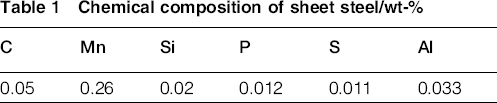
The material welded by the RSW process is sheet steel, whose chemical composition is shown in Table 1. The thickness of the sheet steel is 1 mm.

Table 1

Chemical composition of sheet steel/wt-%

C	Mn	Si	P	S	Al
0.05	0.26	0.02	0.012	0.011	0.033

The steel sheets are welded in a single phase alternating current 50 Hz equipment using water cooled truncated cone electrodes with 5 mm face diameter.

Welding conditions

A total of 330 joints are obtained by the RSW process. Among the different RSW parameters,^{5, 10} welding time, welding current, electrode force, electrode material and treatment applied to electrode material were considered. The values recommend by McCauley et al.¹¹ are taken as reference for the first three parameters (see Table), electrode force is kept constant for all RSW joints, while welding time and welding current take different values avoiding disturbances such as expulsion.^{5, 12} The different electrode materials and treatments are also shown in Table 2.

Table 2

Resistance spot welding parameters

Welding time/s	Welding current/kA RMS	Electrode force/N	Electrode material (RWMA group A*)	Treatment (applied to electrode material)
0.08	4	980.7	Class 2	O61**
0.10	5		Class 3	TH02††
0.12	6			TF00‡‡
0.14	7
0.16	8
0.20
0.24
0.28
0.32
0.36
0.4

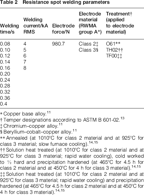
Copper base alloy.¹¹

†

Temper designations according to ASTM B 601-02.¹³

‡

Chromium–copper alloy.¹¹

Beryllium–cobalt–copper alloy.¹¹

Annealed (at 1010°C for class 2 material and at 925°C for class 3 material; slow furnace cooling).^{14, 15}

††

Solution heat treated (at 1010°C for class 2 material and at 925°C for class 3 material; rapid water cooling), cold worked to ½ hard and precipitation hardened (at 465°C for 4.5 h for class 2 material and at 450°C for 4 h for class 3 material).^{14, 15}

‡‡

Solution heat treated (at 1010°C for class 2 material and at 925°C for class 3 material; rapid water cooling) and precipitation hardened (at 465°C for 4.5 h for class 2 material and at 450°C for 4 h for class 3 material).^{14, 15}

Out of the five RSW parameters that are controlled, the electrode force is not regarded as a predictive parameter because its value is kept constant for all RSW joints. Hence, each of the considered classifiers predicts the quality level of RSW joints from four RSW parameters: (i) welding time, (ii) welding current, (iii) electrode material and (iv) treatment applied to electrode material.

Quality levels

The training of the predictive tools employs the 330 joints obtained by RSW process. For each of the RSW joints, the values of the four predictive parameters, which are shown in Table 2, and the quality level, assigned to the RSW joint by a human operator, are used. The quality level may be (i) ‘acceptable’ or (ii) ‘unacceptable’.

The quality level is assessed by ultrasonic testing, except for the cases in which electrode sheet sticking occurs (in 40 out of the 330 total RSW joints); in these cases, the RSW joints are directly considered as ‘unacceptable’ (Fig. 1).

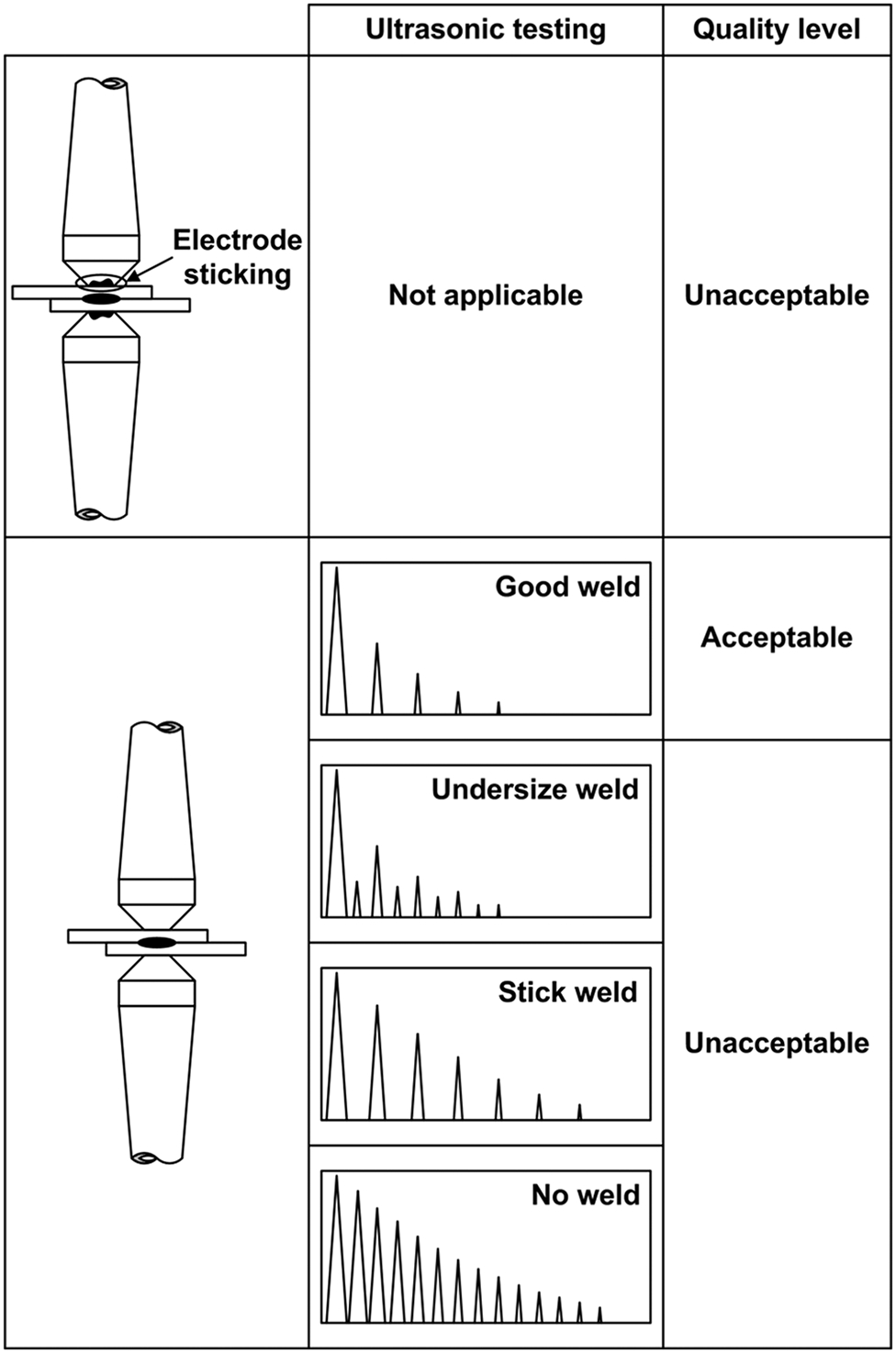
Assessment of quality level of RSW joints by human operator

Since the weld nugget size is the most important parameter among those that determine the mechanical behaviour of the RSW joint,^{16, 17} the quality level assessed by ultrasonic testing must be determined by the size of the weld nugget.¹⁸ The nugget is formed from the solidification of the molten metal and has a cast microstructure with coarse and columnar grains.^{4, 19}

The human operator uses the ultrasonic testing to classify the 330 RSW joints into four categories (Fig. 1) according to the effect of the weld nugget on the ultrasonic beam^{4, 19}: (i) good weld (acceptable quality level): 123/330; (ii) undersize weld (unacceptable quality level): 86/330; (iii) stick weld (unacceptable quality level): 13/330; (iv) no weld (unacceptable quality level): 68/330.

Computational experiments

When a classifier is trained with a given data set, it often overfits the data, especially when using highly flexible models. This means that the classifier learns peculiarities of the training dataset, which are not useful (and may even be detrimental) to predict in a general setting (i.e. when applied to another data set).

A sophisticated family of strategies to conduct model assessment (the evaluation of a model's performance) and model selection (selecting the model with the appropriate balance between flexibility and generalisation ability) is cross-validation (CV). The k fold CV option involves randomly partitioning the original data set into k subsets of approximately equal size, called folds, and use k − 1 of these subsets as training set and the remaining subset as independent test set. This process is then rotated k times, and the results are averaged over the rounds.^{20, 21} This approach is useful because it allows estimating the test error of the classifiers, computing additional measures about the dispersion of the performance and reducing the influence of a particular training/test division in the results. In practice, values of k = 5 and k = 10 have been shown to provide an adequate bias variance trade off without requiring excessive computational power.²¹

It is important to notice that even though CV can be used for model selection and model assessment, some caveats must be considered.²² Several studies^{23, 24} have recently warned against using the error obtained in the selection phase as an estimate of the test error of the selected model (i.e. the error that the model will have on new data). Using several parametric configurations of a classifier and computing the error using CV is adequate to select the right parameters to use, but this error might be too optimistic if reported as an estimate of the performance of the selected model. The estimated errors of the different classifiers analysed in this work have been obtained using a CV scheme suggested as an unbiased estimate of the true performance error of the method. This approach is called nested CV,^{23, 24} although it is also known with other names.²²

Nested CV uses two nested loops: the inner loop is used as model selection in which the parameters are estimated and tested without using all the available data; the outer loop employs the data that have not been used in the inner loop to compute an unbiased estimate of the performance of the model selected in the inner loop. Specifically, the inner loop uses as data the k − 1 folds used as training in the outer loop. These data are in turn used in a k fold analysis for every combination of parameters. For each fold in the outer loop, the model is trained with the combination of parameters with lower error in the inner fold.

In order to compare different classifiers, a performance evaluation metric is required. The most common measure used to assess the performance of a classifier is the percentage of correctly classified data, aka maximum classification rate or accuracy.²⁵ This metric is the proportion of correctly classified data instances in the test sets. Although informative, accuracy is not always the most appropriate measure for comparing classifiers. Among several problems,^{9, 25, 26} perhaps the most relevant in the context at hand is the implicit assumption of equal misclassification costs for false positives and false negatives. When this is not appropriate, the objective function should be a misclassification cost, which weighs false positives and false negatives differently.

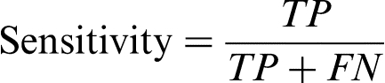
In this work, unacceptable RSW joints are considered positive cases and acceptable joints are considered negative cases. A true positive is an unacceptable joint predicted by the classifier as unacceptable, a true negative is an acceptable joint predicted as acceptable, a false negative is an unacceptable joint predicted as acceptable and a false positive is an acceptable joint predicted as unacceptable. Thus, a high rate of false negative joints can lead to safety problems, while a high rate of false positives can increase the monetary costs of manufacturing and production unnecessarily.

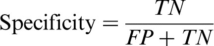
Misclassification costs are often unknown or difficult to estimate, since they depend on the specific industrial objective and are often subject to change. Consequently, comparison among classifiers taking into account both types of errors is decomposed in two complementary performance measures, i.e. sensitivity (the proportion of positive samples that the classifier has correctly identified, equation (1)) and specificity (the fraction of negatives that the classifier has correctly identified, equation (2)), formally defined as 1

Implicitly or explicitly, most classifiers contain a discrimination threshold (e.g. the minimum probability required to classify a sample as positive) that allows them to glide up and down the sensitivity–specificity trade off. A common approach to assess binary classifiers accounting for this degree of freedom is the ROC curve.²⁷ The ROC curve of a classifier shows its true positive rate (or sensitivity) against its false positive rate [i.e. the fraction of misclassified negatives, aka fall out, equal to (1 – specificity)] for different threshold values. The range of possible threshold values is chosen to include both the extreme classifier that classifies all data as negatives (false positive rate = 0, but true positive rate = 0) and the extreme classifier that classifies all data as positives (true positive rate = 1, but false positive rate = 1). The information contained in the ROC curve is often reduced to one single number by computing the area under the (ROC) curve (AUC). The ideal classifier would have a true positive rate equal to one and a false positive rate equal to zero, so the larger the AUC, the better the classifier. An advantage of ROC curves is that they are insensitive to changes in class distribution; hence, this metric has no class skew.²⁷

Classification techniques

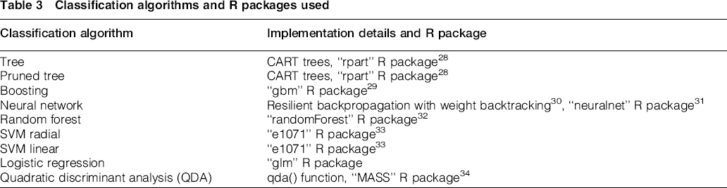
In this work, we have compared the performance of seven classifiers, shown in Table 3, together with the R packages used in the computational experiments. A detailed description of the classification techniques and the parameters used can be found in Supplementary Material 1.

Table 3

Classification algorithms and R packages used

Classification algorithm	Implementation details and R package
Tree	CART trees, “rpart” R package²⁸
Pruned tree	CART trees, “rpart” R package²⁸
Boosting	“gbm” R package²⁹
Neural network	Resilient backpropagation with weight backtracking³⁰, “neuralnet” R package³¹
Random forest	“randomForest” R package³²
SVM radial	“e1071” R package³³
SVM linear	“e1071” R package³³
Logistic regression	“glm” R package
Quadratic discriminant analysis (QDA)	qda() function, “MASS” R package³⁴

Results and discussion

The predictive power of the classifiers has been compared from different perspectives. Nested 10-fold CV has been used to compare the accuracy of the different methods. Table 4 shows the average maximum classification rate of each classifier with its standard error.

Table 4

Duncan's multiple range test and Waller–Duncan's multiple range test for accuracy (α: 0.05)*

Classifier	Accuracy	SE	Duncan subgroup	Waller–Duncan subgroup
RF	0.9576	0.0103	a	a
SVMr	0.9394	0.009035	ab	ab
Boosting	0.9273	0.01979	ab	abc
Logistic	0.9121	0.01313	ab	bc
ANN	0.9121	0.01657	ab	bc
PTrees	0.903	0.01906	b	bc
Trees	0.8939	0.01982	b	c
QDA	0.8455	0.01717	c	d
SVMl	0.797	0.02023	d	e

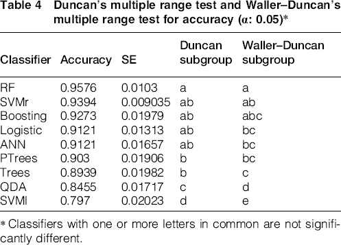
Classifiers with one or more letters in common are not significantly different.

Analysis of variance is used to test the differences in classifier performance. Note that although the accuracy results depicted in Table 4 seem to show differences between classifier performances, these ones could be due to randomness in the training and CV data sets. Table 5 shows the ANOVA results and confirms the statistical difference between classifiers.

Table 5

Analysis of variance of accuracy classifier performance

	Df	Sum sq	Mean sq	F value	Pr(>F)
Classifier	8	0.195	0.02441	8.83	1.3e − 08 ***
Residuals	81	0.224	0.00276

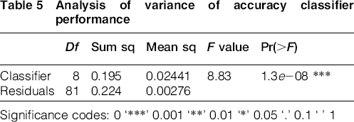
Significance codes: 0 ‘***’ 0.001 ‘**’ 0.01 ‘*’ 0.05 ‘.’ 0.1 ‘ ’ 1

In order to figure out which classifiers are significantly different from each other, Duncan's multiple range test,³⁵ popular in machine learning,⁹ is applied. Apart from using a popular stepwise test such as Duncan's multiple range, we have complemented the comparison using a test that follows a different approach (Bayesian) to determine the significance of the differences: the Waller–Duncan k ratio test.³⁶ This method has good properties from both the Bayesian and frequentist points of view.³⁷ Table 4 shows the classifier performance accuracy sorted in descending order, and grouped into subsets in which performance differences are not significant. Results obtained using Waller–Duncan k ratio test show that the accuracy obtained in previous research using ANN^{8, 19} is outperformed by random forests. However, results from Duncan's multiple range test are not discriminating enough, and the most significant conclusion is that support vector machines using linear kernels exhibit the worst performance. Clearer differences among classifiers are found using AUC performance (Table 8).

As previously discussed, accuracy is not an appropriate performance measure when the cost of a prediction failure – false negative or false positive – is not equivalent. Consequently, the analysis has been complemented comparing the techniques in a wider range of situations using ROC curves and AUC performance. Calculations have been performed with the R package ‘ROCR’, from Sing et al.³⁸ using again a nested 10-fold CV for each classifier. Figure 2 shows the mean ROC curve obtained averaging the 10 folds. Curves intersect, indicating the absence of a dominant classifier for every situation. For instance, Fig. 3 shows that the sensitivity of a gradient tree boosting classifier for a fixed specificity of 75% is similar to a neural network classifier, but is higher when the specificity is fixed to 90% (numeric results can be found in Table 6).

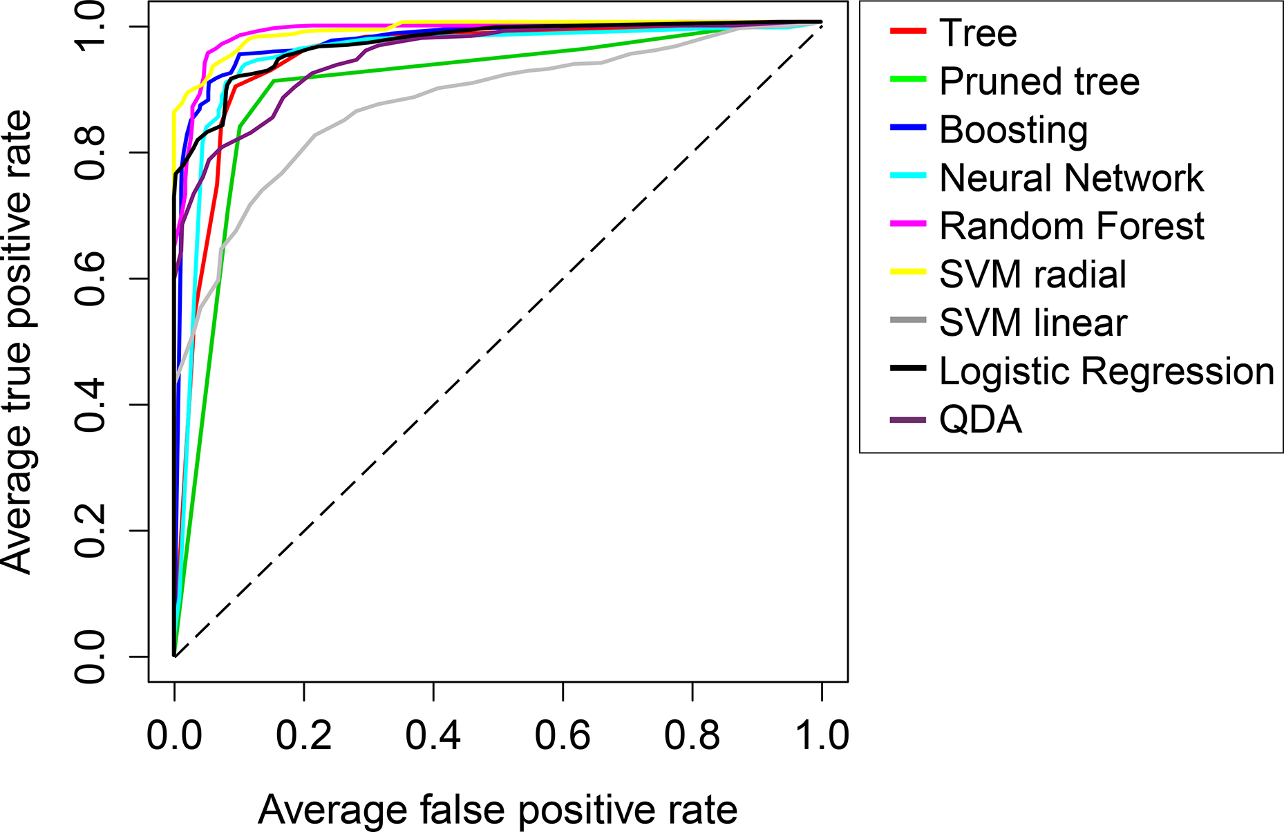
Receiver operating characteristic curve for each tested classifier; dotted diagonal represents random guessing

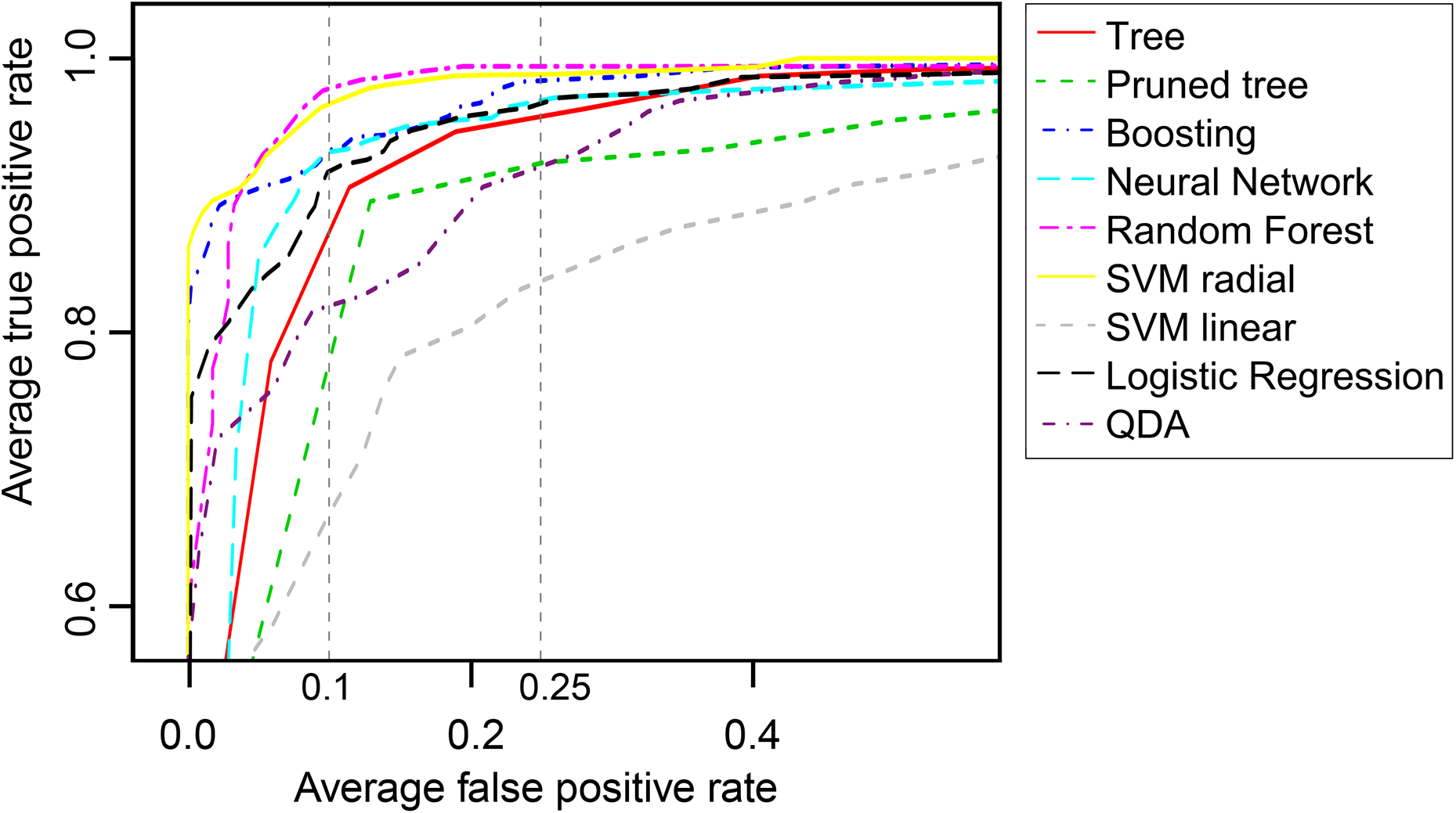
Enlargement of plot in Fig. 2 to show ROC curve for each tested classifier and sensitivity when specificity of 75% or specificity of 90% is required

Table 6

Average AUC, standard error and the sensitivity performance of classifiers when level of specificity is fixed to 75 or 90%

Technique	Area under ROC curve		Sensitivity
Technique	Average AUC	Standard error	Specificity of 75%	Specificity of 90%
Tree	0.9563	0.01274	0.9596	0.8745
Pruned tree	0.9174	0.01888	0.9212	0.7757
Boosting	0.9805	0.0094	0.9816	0.9322
Neural network	0.9448	0.01678	0.9706	0.9322
Random forest	0.9831	0.00631	0.9953	0.9788
SVM radial	0.9899	0.00352	0.9898	0.9651
SVM linear	0.8773	0.01698	0.8361	0.6686
Logistic regression	0.9735	0.00867	0.9706	0.9157
QDA	0.9396	0.01217	0.9212	0.8168

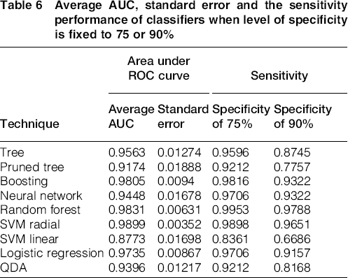
Summarises the average AUC, standard error and the sensitivity performance of the classifiers when a level of specificity is fixed.

Again, results of classifiers using AUC performance are different. An ANOVA has been conducted to test differences in performance (Table 7). Differences are again significant.

Table 7

Analysis of variance of AUC classifier performance

	Df	Sum sq	Mean sq	F value	Pr(>F)
Classifier	8	0.107	0.01333	8.26	4.1e − 08 ***
Residuals	81	0.131	0.00161

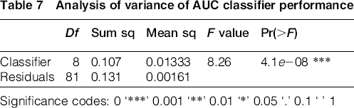
Significance codes: 0 ‘***’ 0.001 ‘**’ 0.01 ‘*’ 0.05 ‘.’ 0.1 ‘ ’ 1

Support vector machines using radial kernel, random forests and boosting obtain again the best overall results (Table 8). Waller–Duncan k ratio test shows that the differences with ANN or QDA are statistically significant; however, the differences obtained with logistic regression or trees are not enough to be considered significant with any of the used tests.

Table 8

Duncan's multiple range test and Waller–Duncan's multiple range test for AUC (α: 0.05)*

Classifier	AUC	SE	Duncan subgroup	Waller–Duncan subgroup
SVMr	0.9899	0.00352	a	a
RF	0.9831	0.00631	a	a
Boosting	0.9805	0.0094	a	a
Logistic	0.9735	0.00867	ab	ab
Trees	0.9563	0.01274	ab	abc
ANN	0.9448	0.01678	ab	bcd
QDA	0.9396	0.01217	ab	cd
PTrees	0.9174	0.01888	bc	d
SVMl	0.8773	0.01698	c	e

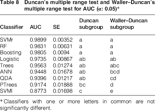
Classifiers with one or more letters in common are not significantly different.

In order to better interpret the effect of the different welding variables in the quality of the RSW joints, the different decision boundaries proposed by the best classifiers – boosting, random forests and SVM radial – are compared in Fig. 4. An analysis quantifying the relative effect of each one of the variables considered for classification can be found in Supplementary Material 2, and a multiclass analysis estimating the types of errors depending on the region can be found in Supplementary Material 3.

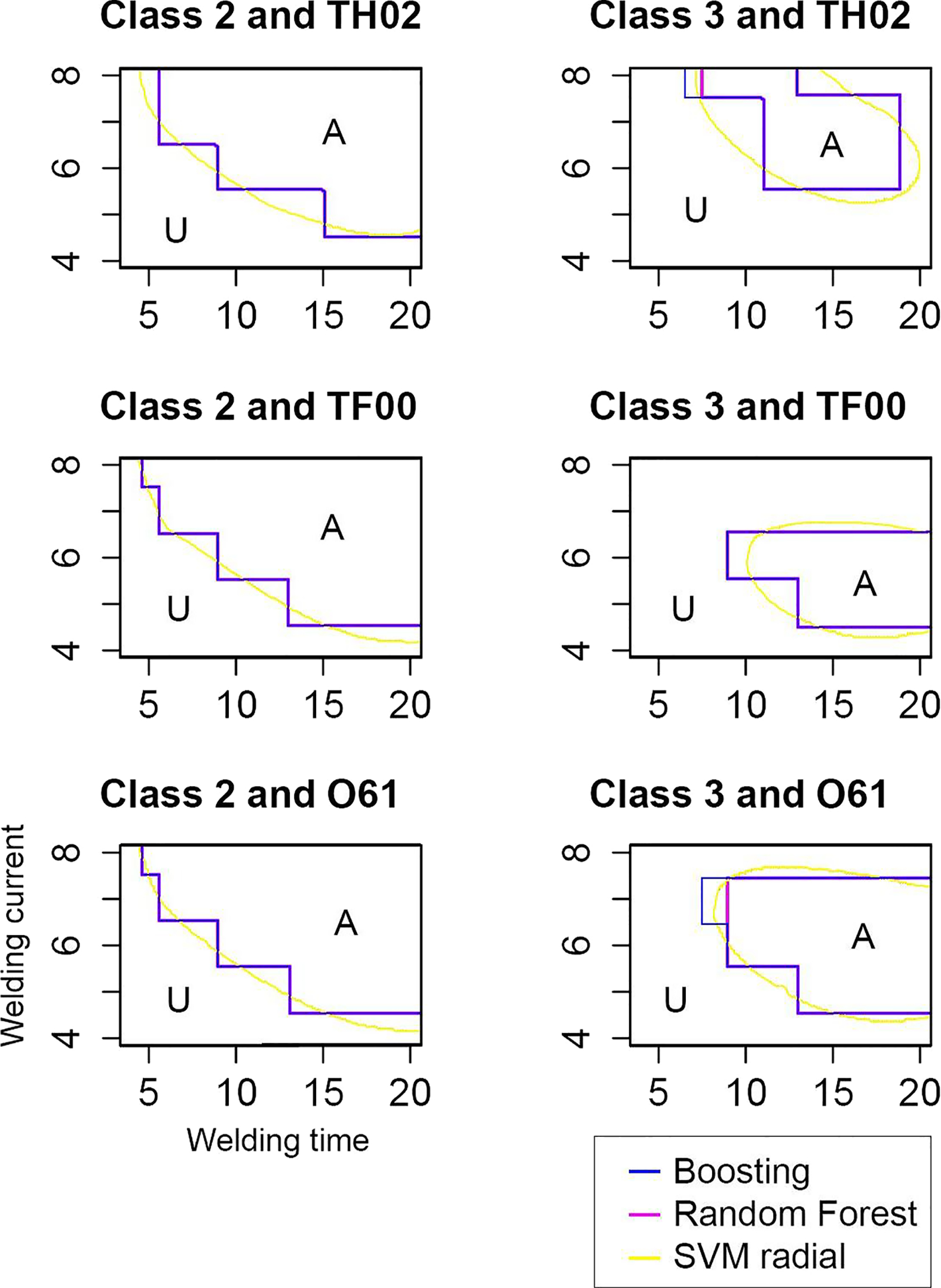
Decision boundaries computed by boosting, random forest and SVM radial algorithms. “A” represents acceptable region, and “U” represents unacceptable region. Welding current, welding time and electrode effects are considered

Class 2 electrode is less sensitive to treatment effects and offers better results than class 3 electrode since it has higher thermal and electrical conductivities.¹¹ On the other hand, class 3 electrode offers better mechanical properties¹¹ that prevent the electrode tip deformation (associated with the increase in the electrode contact face and the consequent current density decrease), which occurs after a prolonged and continuous use. Nevertheless, this better behaviour of class 3 is not shown in results because, in this work, the electrodes are subject to less demanding conditions than those used in automotive industry when high productivity is sought.

In RSW processes, electrodes must have a good combination of (i) sufficiently high thermal and electrical conductivities (to prevent electrode sheet sticking) and (ii) adequate strength (to avoid deformation at high pressures and temperatures).¹¹ TF00 temper can achieve this good combination of physical and mechanical properties because the formation and growth of the strengthening precipitates also reduce the contents of solute atom in matrix, and, hence, the electrical conductivity increases.^{39, 40} This effect is accentuated in TH02 temper where the cold work before precipitation hardening gives rise to dislocations that provide additional nucleation sites at which heterogeneous nucleation can occur. The consequent increase in the density of precipitates for a given time of aging^{41, 42} not only enhances the strengthening but also increases the electrical conductivity. O61 temper, although leads to low mechanical properties, offers good results because, in the present work, the electrodes are not subject to demanding conditions that may cause the electrode tip deformation and the consequent current density decrease.

Conclusions

In this work some of the most relevant and popular pattern recognition techniques have been compared for classification of RSW joints using the welding parameters as inputs. The major conclusions are the following. 1

The analysis confirms that knowing the welding time, the welding current and the type of electrode (electrode material and treatment) is sufficient to obtain classification rates almost comparable with those obtained using non-destructive testing. Additional causes of disturbance can appear during and after the welding process (e.g. electrode degradation, expulsion, current shunting, greasy surface…) but the use of a direct controlling process can reduce significantly the workload of a subsequent quality control. The proposed methodology could be used to implement an anomaly detection algorithm that can warn in real time about potentially detrimental drifts in the welding process. Thus, problematic welding parametric regions could be detected before unacceptable RSW joints appear as a consequence of the direct set-up.

According to Waller–Duncan k ratio test, random forests significantly improve the classification performance (accuracy) obtained by previous research.⁸ These results suggest their use as effective decision support tools to assist directly in quality control of the RSW process, reducing post-welding testing. The differences among random forests, support vector machines using radial kernel and boosting are not found significant.

Results show that for this problem there is not a dominant classifier for every possible pair specificity/sensitivity. An algorithm can perform better than others depending on the industrial context that determines the different cost of a prediction error. Notwithstanding, in an aggregated way, the analysis of the AUC performance measure shows that support vector machines using radial kernel, boosting, random forest and logistic regression using cubic terms or even decision trees are better candidates.

Acknowledgements

The authors would like to thank Dr L. R. Izquierdo for some advice and comments on this paper. The authors acknowledge support from the Spanish MICINN Project CSD2010-00034 (SimulPast CONSOLIDER-INGENIO 2010) and by the Junta de Castilla y León GREX251-2009.

References

Kim

J. H.

, Cho

and Jang

Y. H.

: ‘Estimation of the weldability of single-sided resistance spot welding’, J. Manuf. Syst., 2013, 32, 505–512, DOI: 10.1016/j.jmsy.2013.04.007.

Martín

, López

, De Tiedra

and Juan

M. S.

: ‘Prediction of magnetic interference from resistance spot welding processes on implantable cardioverter-defibrillators’, J. Mater. Process. Technol., 2008, 206, 256–262, DOI: j.jmatprotec.2007.12.021.

Hamidinejad

S. M.

, Kolahan

and Kokabi

A. H.

: ‘The modeling and process analysis of resistance spot welding on galvanized steel sheets used in car body manufacturing’, Mater. Des., 2012, 34, 759–767, DOI: 10.1016/j.matdes.2011.06.064.

Martín

Ó.

, Pereda

, Santos

J. I.

and Galán

J. M.

: ‘Assessment of resistance spot welding quality based on ultrasonic testing and tree-based techniques’, J. Mater. Process. Technol., 2014, 214, 2478–2487, DOI: 10.1016/j.jmatprotec.2014.05.021.

Zhang

H. J.

, Wang

F. J.

, Gao

W. G.

and Hou

Y. Y.

: ‘Quality assessment for resistance spot welding based on binary image of electrode displacement signal and probabilistic neural network’, Sci. Technol. Weld. Joining, 2014, 19, 242–249, DOI: 10.1179/1362171813Y.0000000187.

Parida

and Pal

: ‘Fuzzy assisted grey Taguchi approach for optimisation of multiple weld quality properties in friction stir welding process’, Sci. Technol. Weld. Joining, 2014, 20, 35–41, DOI: 10.1179/1362171814Y.0000000251.

Wong

Y. R.

and Ling

S. F.

: ‘Novel classification method of metal transfer modes in gas metal arc welding by real time input electrical impedance’, Sci. Technol. Weld. Joining, 2013, 19, 224–230, DOI: 10.1179/1362171813Y.0000000184.

Martín

, López

and Martín

: ‘Redes neuronales artificiales para la predicción de la calidad en soldadura por resistencia por puntos’, Revista de Metalurgia., 2006, 42, 345–353, DOI: 10.3989/revmetalm.2006.v42.i5.32.

Bradley

A. P.

: ‘The use of the area under the ROC curve in the evaluation of machine learning algorithms’, Pattern Recog., 1997, 30, 1145–1159, DOI: 10.1016/S0031-3203(96)00142-2.

10.

S. Simoncic, P. Podržaj : ‘Resistance spot weld strength estimation based on electrode tip displacement/velocity curve obtained by image processing’, Sci. Technol. Weld. Joining, 2014, 19, 468–475, DOI: 10.1179/1362171814Y.0000000212.

11.

McCauley

R. B.

, Bennett

M. P.

, Bodary

W. D.

, Farrington

G. C.

, Gasser

R. J.

, Hurd

W. W.

, Schueler

A. W.

, Shearer

T. W.

and Silverberg

J. B.

: ‘Resistance spot welding’, in ‘Metals handbook, vol. 6: welding and brazing’, (ed. Lyman

., 401–424; 1971, Materials Park, OH, American Society for Metals.

12.

P. Podržaj, S. Simoncic : ‘Resistance spot welding control based on the temperature measurement’, Sci. Technol. Weld. Joining, 2013, 18, 551–557, DOI: 10.1179/1362171813Y.0000000131.

13.

601-02

ASTMB

: ‘Standard classification for temper designations for copper and copper alloys-wrought and cast’, 2002, West Conshohocken, PA, ASTM International.

14.

Harkness

J. C.

and Guha

: ‘Beryllium-copper and beryllium-nickel alloys’, in ‘Metals handbook ninth edition, vol. 9: metallography and microstructures’, (ed. Mills

et al.., 392–398; 1985, Materials Park, OH, American Society for Metals.

15.

Joseph

and Kundig

K. J. A.

: ‘Copper: its trade, manufacture, use and environmental status’, 1999, Materials Park, OH, ASM International.

16.

Moshayedi

and Sattari-Far

: ‘Numerical and experimental study of nugget size growth in resistance spot welding of austenitic stainless steels’, J. Mater. Process. Technol., 2012, 212, 347–354, DOI: 10.1016/j.jmatprotec.2011.09.004.

17.

Luo

, Li

J. L.

and Wu

: ‘Nugget quality prediction of resistance spot welding on aluminium alloy based on structureborne acoustic emission signals’, Sci. Technol. Weld. Joining, 2013, 18, 301–306, DOI: 10.1179/1362171812Y.0000000102.

18.

Mansour

: ‘Ultrasonic testing of spot welds in thin gage steel’, in ‘Nondestructive testing handbook. Vol. 7: ultrasonic testing’, (ed. McIntire

., 557–568; 1991, Materials Park, OH, American Society for Nondestructive Testing.

19.

Martín

, López

and Martín

: ‘Artificial neural networks for quality control by ultrasonic testing in resistance spot welding’, J. Mater. Process. Technol., 2007, 183, 226–233, DOI: 10.1016/j.jmatprotec.2006.10.011.

20.

Shao

, Paynabar

, Kim

T. H.

, Jin

, Hu

S. J.

, Spicer

J. P.

, Wang

and Abell

J. A.

: ‘Feature selection for manufacturing process monitoring using cross-validation’, J. Manuf. Syst., 2013, 32, 550–555, DOI: 10.1016/j.jmsy.2013.05.006.

21.

Hastie

, Tibshirani

and Friedman

J. H.

: ‘The elements of statistical learning: data mining, inference, and prediction’, 2009, New York, NY, Springer.

22.

Krstajic

, Buturovic

, Leahy

and Thomas

: ‘Cross-validation pitfalls when selecting and assessing regression and classification models’, J. Cheminform., 2014, 6, 10, DOI: 10.1186/1758-2946-6-10.

23.

Varma

and Simon

: ‘Bias in error estimation when using cross-validation for model selection’, BMC Bioinform., 2006, 7, 91, DOI: 10.1186/1471-2105-7-91.

24.

Anderssen

, Dyrstad

, Westad

and Martens

: ‘Reducing over-optimism in variable selection by cross-model validation’, Chemom. Intell. Lab. Syst., 2006, 84, 69–74, DOI: 10.1016/j.chemolab.2006.04.021.

25.

Viaene

, Derrig

R. A.

, Baesens

and Dedene

: ‘A comparison of state-of-the-art classification techniques for expert automobile insurance claim fraud detection’, J. Risk Insurance, 2002, 69, 373–421, DOI: 10.1111/1539-6975.00023.

26.

Provost

and Fawcett

: ‘Robust classification for imprecise environments’, Mach. Learn., 2001, 42, 203–231, DOI: 10.1023/A:1007601015854.

27.

Fawcett

: ‘An introduction to ROC analysis’, Pattern Recognit. Lett., 2006, 27, 861–874, DOI: 10.1016/j.patrec.2005.10.010.

28.

Therneau

T. M.

and Atkinson

E. J.

: ‘An introduction to recursive partitioning using the rpart routines’ ‘Division of Biostatistics 61’, 1997, Mayo Foundation.

29.

Ridgeway

: ‘Generalized boosted regression models’, Documentation on the R Package ‘gbm’, version 1.5.7 ; 2006.

30.

Riedmiller

: ‘Rprop - description and implementation details, technical report’, 1994;. University of Karlsruhe, Karlsruhe, Germany..

31.

Günther

and Fritsch

: ‘neuralnet: training of neural networks’, The R J., 2010, 2, 30–37.

32.

Liaw

and Wiener

: ‘Classification and regression by random forest’, R News, 2002, 2, 118–122.

33.

Dimitriadou

, Hornik

, Leisch

, Meyer

and Weingessel

: ‘Misc functions of the Department of Statistics (e1071), TU Wien. R package version 1.6-3’, 2008.

34.

Venables

W. N.

and Ripley

B. D.

: ‘Modern applied statistics with S’, 2002, New York, Springer.

35.

Duncan

D. B.

: ‘Multiple range and multiple F tests’, Biometrics, 1955, 11, 1–41, OI: 10.2307/3001478.

36.

Waller

R. A.

and Duncan

D. B.

: ‘A Bayes rule for the symmetric multiple comparisons problems’, J. Am. Stat. Assoc., 1969, 64, 1484–1503.

37.

Shaffer

J. P.

: ‘A semi-Bayesian study of Duncan's Bayesian multiple comparison procedure’, J. Stat. Plan. Inference., 1999, 82, 197–213, DOI: 10.1016/S0378-3758(99)00042-7.

38.

Sing

, Sander

, Beerenwinkel

and Lengauer

: ‘ROCR: visualizing classifier performance in R’, Bioinform., 2005, 21, 3940–3941, DOI: 10.1093/bioinformatics/bti623.

39.

Gao

, Tiainen

, Ji

and Laakso

: ‘Control of microstructures and properties of a phosphorus-containing Cu-0.6 Wt.% Cr alloy through precipitation treatment’, J. Mater. Eng. Perform., 2000, 9, 623–629, DOI: 10.1361/105994900770345476.

40.

J. H.

, Dong

Q. M.

, Liu

, Li

H. J.

and Kang

B. X.

: ‘Research on aging precipitation in a Cu-Cr-Zr-Mg alloy’, Mater. Sci. Eng. A, 2005, A392, 422–426, DOI: 10.1016/j.msea.2004.09.041.

41.

Clark

J. B.

: ‘Age hardening in a Mg-9 wt.% Al alloy’, J. Artic. Acta Metall., 1968, 16, 141–152, DOI: 10.1016/0001-6160(68)90109-0.

42.

Ringer

S. P.

, Muddle

B. C.

and Polmear

I. J.

: ‘Effects of cold work on precipitation in Al-Cu-Mg-(Ag) and Al-Cu-Li-(Mg-Ag) alloys’, Metall. Mater. Trans. A, 1995, 26A, 1659–1671.