Analytical modelling of hysteresis heating in rolling contact of rubber covered rollers

Abstract

In a previous paper, an approximate model for the contact between a rubber covered roller and a rigid roller was developed as analytical functional relationships connecting geometric parameters and material properties of the rubber to nip properties such as maximum contact pressure, etc. in a two-dimensional relationship. The results from that development are used in this work, with the objective to provide a means of estimating the temperature rise due to hysteresis heating. In the heat conduction modelling, one-dimensional steady state heat conduction is assumed. The heat source is a power input coming from internal friction developed during the rolling contact. The power input is expressed by the hysteresis in the rubber represented by a loss angle of the material together with the peripheral speed and some parameters taken from the previously developed contact model. The temperature distribution is calculated in accordance with temperature and heat flow boundary conditions.

Keywords

Rubber covered rollers Rolling contact Hysteresis heating Heat conduction Analytical models

Introduction

The roller contact problem is quite common in applications occurring for example in paper making, copying and printing machines.

The analytical models presented here concern temperature rise and heat flow due to hysteresis heating in rolling contact. This work is a continuation of a previous work by Austrell and Olsson.1

Many other researchers have studied the thermomechanical problem of heat generation in elastomers during rolling. In connection to tyres, a lot of work has been done by using finite elements to solve the coupled mechanical and thermal problem. Park et al.2 and Shida et al.3 have done such work. The latter have used static finite element analysis together with loss factors of the materials to obtain a practical method giving adequate accuracy. This is similar to the work presented here. However, using the equations given here, it is possible to obtain stand alone algorithms from the analytical expressions in order to solve the coupled problem.

Figure 1 shows the roller configuration and parameters. (The paper that passes the nip is not shown in the figure.) Some of the equations for the mechanical problem presented in the previous paper1 are also used in this work. In the previous mechanical part of the modelling, being two-dimensional (2D), the line load q, geometric properties (radius r, rubber layer thickness t and rigid roller radius R) and the shear modulus G are connected to the nip parameters in a functional relationship. These nip properties are the nip width b, indentation u, maximum nip pressure p_max and tangential strain ϵ_t. A master variable from the work of Parish4, 5 is used to set up the relations.

Figure 1

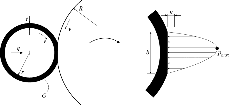
Roller configuration with rubber covered roller and rigid roller: nip properties are shown enlarged to right

In order to determine the heat flow and temperature rise in the rubber layer, some additional parameters such as heat conductivity λ, heat conduction coefficient α and damping properties of the rubber material, are needed. The damping causes mechanical work to become heat. This heating during rolling contact can be estimated from the loss or phase angle of the rubber material and from approximate relationships for the deformation. The hysteresis work per unit time in the rubber is a heat power supply causing the temperature to rise in the rubber layer. This source term in the heat equation is discussed in the section on ‘Heat source’.

Experimental data for the rubber material obtained in harmonic shear tests are used to define material parameters needed for the calculations. The experimentally obtained dynamic stiffness and phase angle are used together with estimated heat conduction properties as input in the models according to the section on ‘Mechanical parameters’.

By solving the heat equation as described in the section on ‘Heat transfer model’, an estimate of the temperature rise in the rubber can be obtained. The heat conduction part of the modelling uses a one-dimensional (1D) steady state model with the hysteresis as the heat source. The boundary conditions in the heat equation are formulated as temperature and flow conditions taking the cooling by air, paper and water into account, as described in the section on ‘Cooling sources’.

The models presented here and in the previous work1 have been implemented in MATLAB6 giving the nip properties, hysteresis power supply, heat flow and temperature rise as output. Some examples of output are shown in the section on ‘Examples of parameter dependence’.

Heat source

An expression representing the heat source is presented in this section, making it possible to calculate the power input generated by hysteresis work. The derivation is starting from an expression of harmonic steady state hysteresis work of linear viscoelastic materials. This expression is adapted to fit the loading in roller applications that can be described as periodic transients of approximately half-sinusoidal shape occurring once in every revolution for a particular point in the rubber layer, schematically illustrated in Fig. 2.

Figure 2

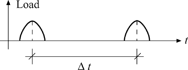
Loading in rolling contact following point on periphery of rubber covered roller: Δt is time for one revolution

The basic expression used for estimating the hysteresis heating is as mentioned an expression valid for the harmonic case, illustrated in the left part of Fig. 3. The heat generated in a specimen loaded harmonically (i.e. with a sinusoidal load) is dependent on the stress and strain amplitudes σ₀ and ϵ₀ and on the loss angle δ (in radians) according to the hysteresis work expression (1) with the hysteresis work U_c as energy per cycle and unit volume (i.e. J m⁻³). This expression is, however, valid for a completed cycle, i.e. U_c is the energy developed per unit volume for one stress–strain cycle. For a pulse starting from zero (as for the loading discussed above, see Fig. 2), only a fraction of the energy contributes to the heating of the rubber. Looking at the shaded area in Fig. 3 yields that this area equals approximately one-third of the area enclosed by the complete loop.

Figure 3

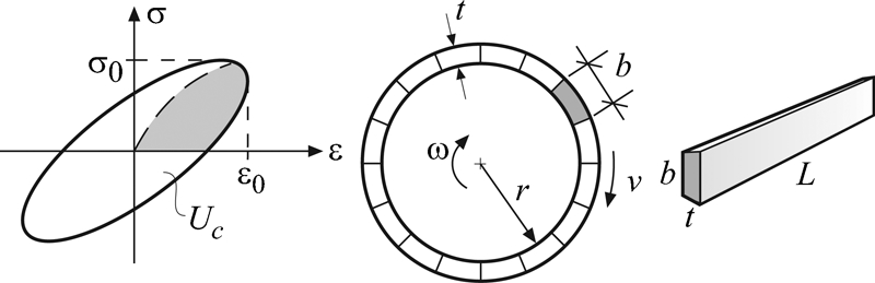
Stress–strain loop for viscoelastic material with loss angle δ (left) and rubber layer divided in strips of width equal to nip width (right)

Furthermore, one imagines the rubber layer on the roller divided in strips of the same width as the nip width b and assumes that the hysteresis heating discussed above is developed in one strip at a time while the roller is rotating with an angular frequency ω, according to Fig. 3.

The power P in the entire rubber layer can then be calculated by looking at the number of strips around the roller and the angular velocity of the roller. The energy (in J) developed during one revolution is expressed by recognising that the number of strips around the perimeter is 2πr/b and the volume of each strip is btL (L is the length of the roller) giving (2) The energy per radian is easily calculated by dividing by 2π. Then by multiplying with the angular velocity ω, the power P generated by hysteresis in the rubber layer is P = U_cLtωr/3. Also using the speed of the periphery ν = ωr, the power generated can be expressed as (3) giving the heat input power due to hysteresis.

Now, σ₀ and ϵ₀ in U_c need to be expressed in other variables in order to be useful here. Owing to equilibrium of forces, the mean pressure in the nip p_mean can be expressed as (4) by using the line load q (in N m⁻¹) and the nip width b. This can be seen from the force on the roller F = qL and observing that F/A = qL/(bL) giving the expression above if A is the area covered by the nip. By putting σ₀ = p_mean = q/b and ϵ₀ = u/t, the heat input power expression can now be written (5) with the power P (in W), line load q, indentation u, nip width b, peripheral speed v (in m s⁻¹), phase angle δ (in radians) and L (could be set to 1 m). The parameters included in equation (5) will be discussed next.

Mechanical parameters

In the hysteresis power expression equation (5), u and b need to be calculated. This can preferably be done by the functional relationships of the 2D contact model described in Ref. 1 for roller nip analysis, using the input variables q, r, R, t and G (according to the section on ‘Introduction’). In order to put in a representative value of the shear modulus G, one should consider the influence of loading rate, amplitude and temperature. This is also the case for the phase angle used in the power expression equation (5). The shear modulus and the phase angle dependence on these three variables can be experimentally determined by for instance a harmonic sinusoidal shear test. However, in order to use the experimental data in this application, one needs to translate the shear strain used in the experiments to compressive strain which is dominating in the roller nip. This can be done using an energy equivalent translation from shear strain κ to compressive strain ϵ. Putting energies equal (6) and using Young's modulus E≈3G due to incompressibility, the experimental shear strain to be used is found to be κ₀ = 3^1/2ϵ₀. Here, the previously defined (roller) nominal compressive strain ϵ₀ = u/t is translated into the experimental shear strain κ₀.

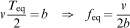
Moreover, one needs to translate the loading rate occurring in the roller application to an equivalent loading rate to be used in the shear strain test. An estimate of the loading rate from the perimeter speed v and the nip width b yields the equivalent frequency f_eq used for finding the correct value of G_dyn and δ from experiments. Again using the similarity of the nip profile and a half-sinusoidal period of experimental straining, one get with time T_eq = 1/f_eq (7) In summary, the experimental shear test data for a suitable temperature T at the shear strain amplitude κ₀ and experimental frequency f_eq yield G_dyn and δ to put into the 2D elastic contact model1 and the power expression equation (5).

Heat transfer model

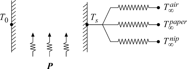
The geometry for the heat transfer model is schematically illustrated in Fig. 4, showing to the right a small part of the rubber cover. At the left boundary is the metallic core and at the right boundary is the air outside the rubber layer. Heat is generated inside the rubber (according to the power expression) and is flowing inward and outward through the rubber layer.

Figure 4

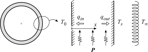
Part of rubber layer giving geometry of 1D heat transfer set-up, with heat source, heat flow and boundary temperatures: to the right, convective layer is illustrated with rubber surface temperature T_s on one side and air temperature T_∞ on the other

A simple steady state model for the temperature part is used. For the heat conduction in the rubber layer, according to Fig. 4, an approximate 1D heat transfer analysis is employed. The assumption of steady state is of course an approximation, as the heat generation is spinning around the periphery of the rubber layer. The point of contact changes and there is cooling in between the contact of the rubber nip. However, it is a fast moving source and the variations in the source due to the rotation should not be too big, justifying the assumption.

The hysteresis heating according to the discussion above is regarded as a uniformly distributed heat source through the thickness. This is a simplifying assumption and it is also an approximation, as the true source distribution has a maximum somewhere inside the rubber layer.

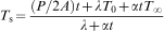
In order to correctly define the heat conduction problem in the rubber layer, the boundary temperatures or flows need to be specified. The boundary condition on the left hand side is easy to set up as it can be defined as a temperature condition. The rubber covered roller has a metal core with a given temperature T₀. On the right hand side, it is assumed that the surface temperature T_s is constant on the periphery as shown in Fig. 4. At the outside, several estimates regarding the cooling have to be considered. The periphery of the rubber covered roller is divided in three parts: one is open to and cooled by the surrounding air, a second is covered by paper and the third part is defined by the roller nip. These resistances are discussed in more detail in the section on ‘Cooling sources’.

As mentioned above, the heat conduction is for simplicity treated as a steady state 1D problem and the heat source is regarded as an evenly distributed source through the thickness of the rubber. In order to formulate the heat conduction problem, Fourier's law according to (8) is used, with heat flow q_h (in W m⁻²), temperature T (in K), position x in the thickness direction and thermal conductivity λ (in W m⁻¹ K⁻¹). The evenly distributed heat source will give a parabolic temperature distribution in the rubber layer with thickness t according to Fig. 5.

Figure 5

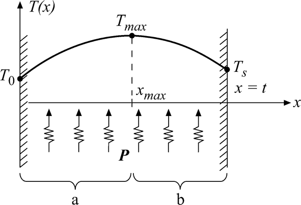
Parabolic temperature distribution in rubber layer and maximum temperature and its location in rubber layer

The heat input power P will flow inward and outward through the left and right boundaries respectively, also illustrated in Fig. 4. The energy balance for this heat flow can be written as (9) It is assumed that the area A = 2πrL for flow inward and outward is the same. The boundary condition to the right is written as a convective flow condition (10) with the flow controlled by the convection coefficient α (in W m⁻² K⁻¹) and the temperature difference in the convective layer (see Fig. 4).

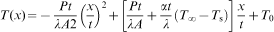
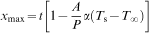
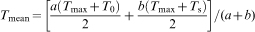
Using the boundary conditions, the temperature distribution T(x) is found by solving the heat equation, giving (11) the quadratic temperature distribution expressed in terms of the parameters at hand. Particularly at the right hand side boundary (putting x = t), the temperature is (12) with P being the power input from hysteresis. It is also of interest to know the maximum temperature T_max occurring in the rubber layer as illustrated by Fig. 5. The maximum temperature occurs at (13) giving the temperature from the general expression as T_max = T(x_max).

Finally, the mean temperature is also a quantity needed in the section on ‘Temperature calculation strategy’, This temperature can be written as (14) by using a weighted sum of quantities already calculated. Here it is assumed that a = x_max and b = t−x_max.

Cooling sources

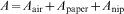
Consider the right hand side of the heat transfer model, i.e. the outside boundary. In this section, the cooling due to the outgoing heat flow will be discussed. This resistance for the outgoing heat flow is by convection to air, the contacting paper track and the nip (see Fig. 6).

Figure 6

Cooling by convection

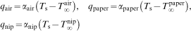
The outgoing heat flow is divided into three parallel parts according to (15) with A = 2πrL and the corresponding surfaces fulfilling (16) Writing the resistances as convection boundary conditions yields (17) For simplicity, in order to evaluate the influence of different terms, and also being a reasonable assumption, put (18) Inserting this into equation (15) yields (19) and by collecting things as (20) the parallel heat flow can be replaced with one resistance having α_eq as the convection coefficient. The α in the previous section on ‘Heat transfer model’ should be replaced by the value above.

Temperature calculation strategy

The heat calculation strategy (using MATLAB) is described here as a summary of the previous discussion:

the calculation starts with a good guess of G_dyn = G_dyn(f, κ, T) as a function of frequency, shear strain and temperature using the experimental shear strain data

ii.

from the initial guess on G_dyn, a nip width b and an indentation u are calculated using the 2D contact model

iii.

the nip width is used to give an estimate of the loading rate in terms of an equivalent frequency from the perimeter speed v as f_eq = ν/2b

iv.

the indentation is used to give an estimate of an equivalent shear strain κ using also the thickness t of the rubber layer as κ = 3^1/2u/t.

The last two expressions are according to the section on ‘Mechanical parameters’ above.

from the experimental shear strain data, a phase angle δ corresponding to the guess of dynamic modulus is used, together with other parameters, to estimate the hysteresis power P generated (21) This was discussed in the section on ‘Heat source’ above.

vi.

now, using the heat conduction equations, a temperature distribution T = T(x) can be calculated according to the section on ‘Heat transfer model’. In that section, an expression for the mean temperature T_mean in the rubber layer is also given

vii.

by using the calculated set of parameters κ, f_eq and T_mean, it is possible to obtain new values for the dynamic shear modulus G_dyn and phase angel δ from the experimental data.

Repeating the steps above yields an iteration procedure that converges when the changes in G_dyn and δ are small enough.

Examples of parameter dependence

In this section it is shown how different parameters influence the temperature in the rubber layer. The start values for all the necessary parameters in these examples are:

geometry: r = 0·15 m, R = 0·3 m and t = 20 mm

ii.

material: G_dyn = 15 MPa and δ = 0·2 rad

iii.

heat conduction parameters: λ = 0·2 W m⁻¹ K⁻¹ and α = 50 W m⁻² K⁻¹

iv.

boundary temperatures: T₀ = 20°C and T_∞ = 25°C

periferal velocity: v = 7·5 m s⁻¹

vi.

line load: q = 50 kN m⁻¹.

The thermal conductivity λ given above is a typical value for rubber and for the convection coefficient α, the value is reasonable if air is the only cooling source.

Using these values in the scheme described yields the following thermal output; maximum (interior) temperature T_max = 68·9°C, surface temperature T_s = 46·9°C and power generation per meter roller P/L = 2·57 kW m⁻¹.

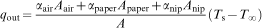
Variations for one parameter at a time around the values above are shown in Figs. 7–10. The small circles shown in the figures are according to the start values above. The upper curves show maximum temperatures T_max in the interior of the rubber layer and the lower curves show temperature at the surface T_s. The figures show these temperatures as functions of thickness t, velocity v, shear modulus G and phase angle δ. The same temperature range is used in all figures to show more clearly the influence of each parameter. Figure 6

Figure 7

Temperatures: maximum (interior) and surface temperature as function of rubber thickness

Figure 8

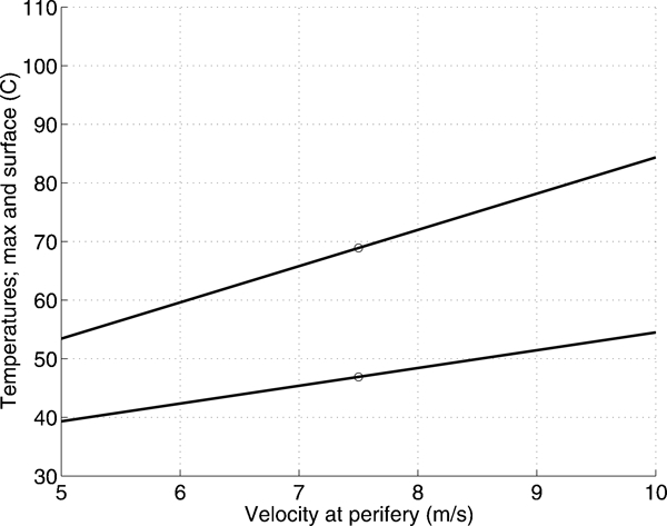
Temperatures: maximum (interior) and surface temperature as function of periferal velocity

Figure 9

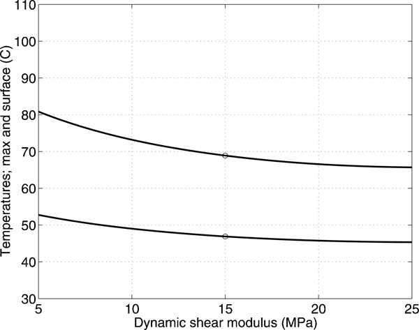
Temperatures: maximum (interior) and surface temperature as function of dynamic shear modulus

Figure 10

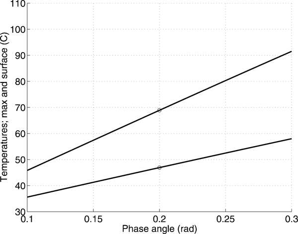
Temperatures: maximum (interior) and surface temperature as function of phase angle

Not surprising, it is seen that thickness and phase angle have great influence on temperature. It can be concluded that bad combinations of parameters easily yield a very high and destructive temperature rise in the rubber layer.

Conclusions

The roller problem discussed here is relevant in many applications. A short description of how the complex problem of estimating temperature rise in rolling contact can be addressed in an approximate way, using analytical expressions, was presented. The motivation for the work is to get a fast way to determine essential thermal parameters in the roller problem without complicated coupled finite element analysis.

References

Austrell

, Olsson

: ‘Two dimensional elastic contact model for rubber covered rollers’, Plast. Rubber Compos., 2013, 42, 7, 269–275.

Park

, Youn

, Song

, Kim

: ‘Analysis of temperature distribution in a rolling tire due to strain energy dissipation’, Tire Sci. Technol. , 1997, 25, 214–228.

Shida

, Koishi

, Kogure

, Kabe

: ‘Rolling resistance simulation of tires using static finite element analysis’, Tire Sci. Technol. , 1999, 27, 84–105.

Parish

: ‘Measurements of pressure distribution between metaland rubber covered rollers’, Br. J. Appl. Phys. , 1958, 9, 158–161.

Parish

: ‘Calculation of the behaviour of rubber-covered pressure rollers’, Br. J. Appl. Phys. , 1961, 12, 333–336.

‘MATLAB reference guide’, The MathWorks Inc., Natick, MA, USA.