Two-dimensional elastic contact model for rubber covered rollers

Abstract

A model for the contact between a rubber covered roller and a rigid roller was developed using analytical functions. The model, being two-dimensional, connects the line load, geometric properties (roller radii, rubber thickness) and the shear modulus of the rubber to nip properties in the roller contact. The output from the model is the indentation of the rigid roller into the rubber, the nip maximum pressure, the nip width and the surface strain in the centre of the nip. Moreover, the shape of the pressure distribution is also given as an analytical expression. The basic assumption relies on the work of Parish (−58 and −61), but a development of this work was performed, showing the influence of the rubber shear modulus and also how the surface strain in the nip can be described. The functional relationships are based on least squares fitting of analytical functions, depending on two master variables, to a large number of finite element analysis results.

Keywords

Rubber covered rollers Contact Nip properties Analytical expressions Fit to FE-results Pressure profile

Introduction

Rollers are used in many applications, in paper making machines, copying machines, in various industrial processes, etc. The objective of this work is to facilitate the future development of rollers by presenting a model that makes it easy to study the effect of changes in the roller configuration, here being a rubber covered roller and a rigid roller. This is accomplished by an analytical expressions showing how parameters in the configuration are affecting the contact between the rollers. Several authors have studied cylinder contact with finite elements (FEs) both quasi-static and in rolling contact, see for example Refs. 1 and 2. However, no literature was found using the approach here, i.e. to establish analytical expressions by interpolation of FE results in the cylinder contact problems.

The modelling discussed here take its departure from the work on rolling contact by Parish.3, 4 While Parish made physical experiments, the experiments here are numerical. Finite element analysis for a large number of roller configurations are forming the basis for the functions involved, which provide an interpolation between results from the FE runs. Thereby the model can also be used to study other combinations of parameters than those used in the FE analysis. Also, the functions used are monotonic, giving reasonable behaviour outside the fitted interval to some extent.

A two-dimensional model of the contact between the rubber covered roller and the rigid roller was developed with the basic assumption that the rubber covered roller behaves elastically and that the conditions are constant along the roller. By this assumption, only a cut plane through the roller needs to be considered.

Moreover, the FE analysis was carried out as a quasi-static analysis, pressing a sector of the rigid roller radially into a sector of the rubber covered roller. This yields a symmetric pressure distribution in contrast to the slightly asymmetric distribution found in dynamic rolling conditions taking the hysteresis of the rubber into account. There are two main deviations of nip properties for the model presented here and the situation in practice, having rolling contact and a real rubber vulcanisate that always exhibits some material damping. The first is due to a general property of dynamically loaded rubber. In dynamic loading the shear modulus is higher compared to the quasi-static case. This can be compensated for by using a dynamic shear modulus obtained from say a sinusoidal double shear test. More about that can be found in Ref. 5. The other deviation is due to material damping. Consider again Fig. 1. Suppose that the rubber covered roller is turning clockwise. Then, there will be a continous loading of the rubber layer in the upper part of the nip and unloading in the lower part. This will yield a slight shift upwards in the location of the maximum pressure due to the simple fact that loading is stiffer than unloading due to hysteresis caused by material damping.

Figure 1

Design and response variables

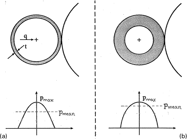
Having these limitations in mind, with the model, one can see how variations of rubber material shear modulus G, thickness of the rubber layer t, rubber covered roller radius r, rigid roller radius R and the line load q (see Fig. 1a) are affecting the contact between the rubber covered roller and the rigid roller. The model provides a link between these input variables for a given design and the variables that describe the nip properties. These output or response variables are the nip width b, indentation u, maximum pressure p_max and the tangential strain ϵ_t of the rubber surface at the centre of the contact (see Fig. 1b).

The relationship consists of analytic functions, linking the response variables to the design variables, and it can schematically be described by (1) (2) (3) (4) In the section on ‘Nip properties using master variables’, there is a more detailed account of the functions and the input variables are reduced by using only two master variables. As mentioned, the functions were generated by fitting to results from FE analysis. A large number of FE calculations with variations in the input parameters, were performed to form the basis for the functional relationships. The functions were fitted with the least squares method by using monotone functions as described in the section on ‘Fitting analytical models to FE results’.

In addition to the relationship above (equations (1) and (3)), giving only the maximum pressure and the nip width as information of the pressure distribution, a more detailed picture of the pressure distribution in the nip is also sought. This is addressed in sections on ‘Pressure distribution in nip’ and ‘Fitting analytical models to FE results’.

The functions have been implemented in MATLAB6 to facilitate the future development of rollers.

Finite element analysis

A total of 405 FE calculations were performed in ABAQUS giving the basis for the analytical model. The rubber covered roller was modeled as a rubber layer on a rigid surface. Since the analysis is static, the drum does not rotate, which means that only a small segment of the roller needs to be modeled (cf. Fig. 2). The rigid roller was also modeled by only a small segment as a rigid surface. Plane strain is used in the analysis, because the rollers are assumed to be much longer than their diameter, giving a reasonable approximation that significantly reduces the evaluation time. The elements were four node hybrid elements CPE 4H. Full integration implicit analysis (ABAQUS Standard7) for large deformations and incompressible conditions was used.

Figure 2

Finite element mesh modelling contact between rubber covered roller and rigid roller

The material behaviour was modelled by a hyperelastic Neo-Hooke model. This simple model works well for rubber at moderately large deformations in compression and shear. It is also easy to determine the material parameter C₁₀, which is equal to G/2, i.e. half the shear modulus.

Calculations were carried out with input data in Table 1, where the range of the shear modulus is corresponding to a rubber hardness of about 65–95 HSA.

Table 1

Range of input parameters for FE calculations

100 mm<r<250 mm

280 mm<R<490 mm

3 mm<t<25 mm

2 MPa<G<30 MPa

20 N mm⁻¹<q<70 N mm⁻¹

The FE analysis was carried out using zero friction in the contact between the rigid and the rubber covered roller. In various applications, friction will vary a lot from about zero in the case when for example some kind of lubricating fluid is present to higher values in dry contact. However, using zero friction yields limiting values of the nip (response) variables. With friction the contact will appear stiffer, giving higher maximum pressure, smaller nip width, smaller indentation and smaller surface strain. Study of the frictional influence is a parametric study in itself and this has not been carried out in this work.

The maximum nominal compressive strain ϵ = u/t is about 13–14% and it is obtained from the extreme case of a soft material (G = 2 MPa) and a high line load (q = 70 N mm⁻¹). The highest values of nominal strain is found for the thinnest (t = 3 mm giving 13%) and the thickest (t = 25 mm giving 14%) rubber layer. These levels of strain justifies the choice of the neo-Hooke model. Even a linear elastic incompressible model would give reasonable results in most cases. Examples showing values of the nip variables as functions of some chosen design variables are shown in the section on ‘Examples: parameter dependence’.

Nip properties using master variables

The roller contact is defined by equations (1)–(4) that show the wanted relationship, consisting of five input parameters and four output parameters. All these nine parameters were shown previously in Fig. 1.

According to early work by Thomas and Hoersch8 on contact in plain strain between a homogeneous elastic roller and a rigid roller, the nip width b₀ in the incompressible case, is given by (5) where (6) In this expression, the nip width dependence of the radii is simplified by introducing the variable D.

Parish used b₀ in his work3, 4 and formed a dimensionless variable (7) to be used in the case of rubber covered roller with an elastic layer of thickness t. Based upon experimental work on soft rubber covered rollers he presented curves being dependent only on X, giving expressions for the maximum pressure, nip width and indentation.

In this work, where the experiments were replaced by FE analysis using much harder rubber materials than used by Parish, it was found that there was a need for another master variable. The curves that were given by Parish as a single curve turned out to be dependent on the shear modulus of the rubber. The dimensionless variable (8) where G₀ = 1 MPa (arbitrary) was introduced because the numerical experiments discussed in the section on ‘Fitting analytical models to FE results’ showed the necessity for it. The functional relationships in equations (1)–(4) can then be expressed as (9) (10) (11) (12) with the maximum pressure (equation (11)) being dependent on the previously calculated nip width (equation (9)). The expression for the surface tangential strain ϵ_t (equation (12)) was not discussed by Parish. It was found during the analysis of the FE results. Using the functions in equations (9)–(12), the variable dependence is thus reduced from five to two variables, making the fit to the FE results, discussed in the section on ‘Fitting analytical models to FE results’, much easier.

Pressure distribution in nip

It is sometimes of interest to know the pressure distribution in the nip and how it varies with different input data parameters. A steep gradient in the beginning of the nip can sometimes be useful in order to squezze out liquids or preventing air from entering the nip.

The consequences of thin and thick layers in combination with the line load are shown in Fig. 3. The pressure profile depends on the thickness of the rubber layer and on the line load. A thin cover and a high line load yields a more triangular shape of the pressure profile and a thick cover yields a more blunt or rounded profile.

Figure 3

Influence of rubber cover thickness t on shape of pressure profile is shown in two extreme cases

The pressure distribution can be obtained using the previously derived maximum pressure p_max in equation (11) and the mean pressure (13) that is from equilibrium reasons the same as the line load divided by the nip width.

The pressure is denoted by p(x) and thus varies with the position x. Figure 4a shows how a pressure distribution might look like and Fig. 4b shows a normalised pressure distribution.

Figure 4

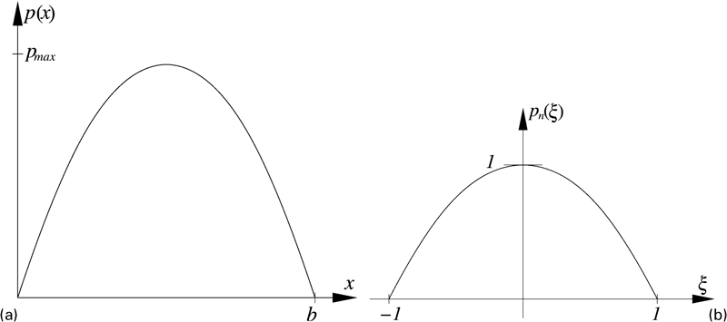
a pressure distribution in contact between rollers and b normalised distribution

The pressure distribution is obtained from a normalised distribution by the equation (14) with (15) An empirical expression for the normalised pressure distribution is fitted to FE results in the section on ‘Fitting analytical models to FE results’.

Fitting analytical models to FE results

Now, in equations (9)–(12) the variable dependence is thus reduced from five to two variables. Using the results from FE analysis, the functions f_b, f_u, f_p and f_ϵ were determined by interpolation. First, the functions were adapted with respect to X with discrete values of Y, and then the functions for Y were fitted, using the least squares method to monotone functions. The advantage of monotonic functions is that they also give an approximate behaviour outside the parameter range used in the fit. In this case, the range of parameters used in the FE calculations are shown in Table 1.

Basic nip functions

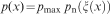
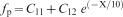
In order to establish suitable functions for the relationships in equations (9)–(12) functions giving the behaviour with respect to X was first sought by looking at Figs. 5 and 6. Points in the figures are results from FE calculations. The influence of the parameter Y is weaker and was fitted in a second step. For the function f_p, no dependence of Y could be sorted out.

Figure 5

Graph of functions f_b and f_u: plotted points are results from FE calculations

Figure 6

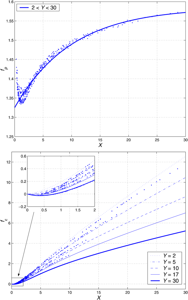
Graph of functions f_p and f_ϵ: plotted points are results from FE calculations

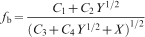
By several numerical experiments the following monotone functions proved empirically to work well. The nip width function (16) the indentation function (17) the pressure function (18) and the surface strain function (19) contain constants C₁–C₁₈ to be determined by least squares fitting to the FE results. Some of the constants appear in a linear fashion and are solved for in the standard way without iterations. The constants that have a non-linear dependence have to be solved for in a loop for a range of assumed values until the minimum solution for the square of the errors are found.

The functions that constitute the analytical calculation model are compared with the results from FE analysis to determine how well they fit to the FE results. Figures 5 and 6 illustrate the functions of equations (16)–(19) for different values of X and Y.

The amounts of the relative errors between the FE calculations and corresponding results with the analytical model are in general small. For the nip width b and the maximum pressure p_max, the errors never exceeds 3 and 6% respectively, but are in general less than 2%. The amounts of the relative errors for the indentation u and the tangential strain ϵ_t are larger. The errors are at its worst 12 and 24% respectively for some values of small X values, but are in general less than 5 and 10% respectively. For small values of X, i.e. when X→0, then f_u→0 and f_ϵ→0 (see the zoomed diagrams of Figs. 5 and 6) the relative errors get big. But the errors are, as mentioned, only large for values of X near zero and this is only the case for some combinations of the limiting values in Table 1.

Pressure distribution function

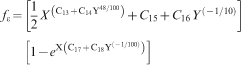
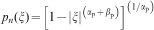
The normalised pressure distribution p_n(ξ) is illustrated in Fig. 4b and can be described empirically as (20) with (21) and β_p and C₁₉–C₂₁ are known constants determined by least squares fitting. The pressure curve is then symmetric around x = b/2 at a static contact between the rollers. The parameter α_p tells what type of distribution the pressure has. Low values give a sharp curve, while high values produce a blunt form of p(x). By looking at extreme combinations of line load and rubber thickness, according to the discussion above, the constants could be determined. (In the work of Ref. 8, a pressure distribution using α_p = 2 and β_p = 0 is used.)

Figure 7 shows the consequence of different values of the quiotent p_mean/p_max according to equation (21), giving a set of normalised pressure distributions. The physical pressure distribution is found from the normalised distribution according to equations (14) and (15).

Figure 7

Examples of normalised pressure distributions

Examples: parameter dependence

In this section, some example of the previously derived functional relationships are presented in terms of nip variable parameter dependence and extreme pressure profile appearance.

Nip variable dependence on two design variables

Here are examples showing the parameter dependence of the nip properties. It was found that the parameters influencing the nip variables the most were the rubber thickness t and the shear modulus G. In order to show the influence of these important parameters, values of the five input (or design) parameters were first taken in the middle of the intervals given by Table 1. Accordingly the following values were choosen: r = 175 mm, R = 385 mm, t = 14 mm, G = 16 MPa and q = 45 N mm⁻¹. In the first example, the thickness t was varied, while the other parameters were kept constant at these values. Figure 8 show the influence of the rubber layer thickness on all four nip variables.

Figure 8

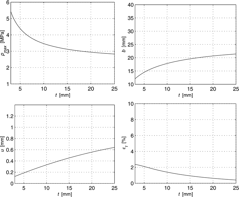
Influence of rubber thickness t on maximum contact pressure p_max, nip width b, indentation u and tangential surface strain ϵ_t

It can be seen that maximum pressure and surface strain is decreasing with increasing thickness and that nip width and indentation is increasing with increasing thickness.

The second example, according to Fig. 9, concerns (as mentioned) the influence of the shear modulus G. The same constant values of the design parameters are used in this example, but now the shear modulus is varied. The four nip variables are plotted in the same scale as in the previous example, to make the comparison easier.

Figure 9

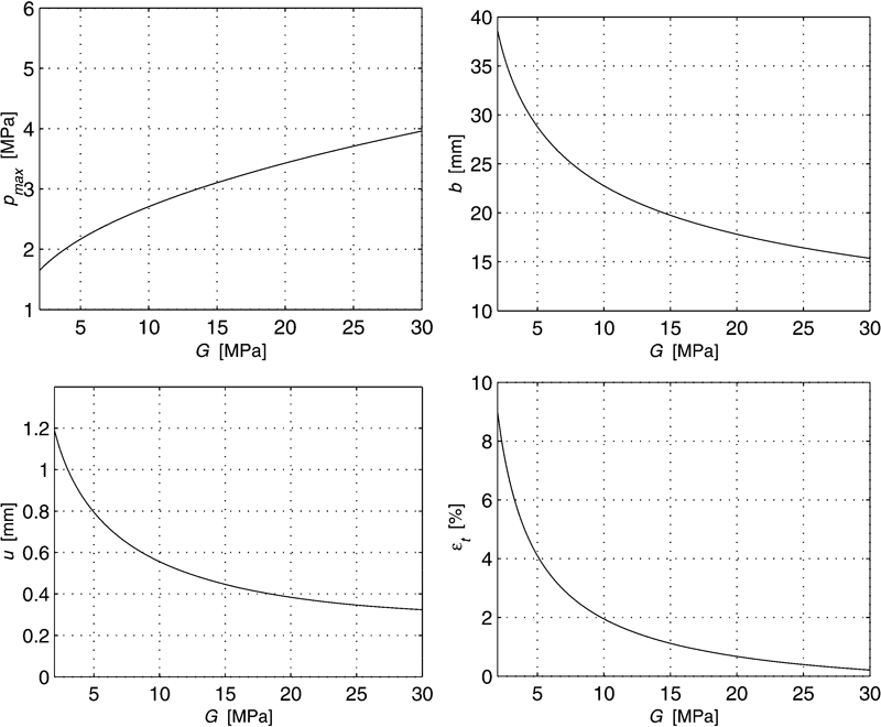
Influence of rubber shear modulus G on maximum contact pressure p_max, nip width b, indentation u and tangential surface strain ϵ_t

Rubber shear modulus affects mostly the result of all parameters. An increase in the modulus provides higher maximum pressure and a reduction in nip width, the indentation and the tangential strain. Dramatic changes can be seen in the three later diagrams when compared with the changes caused by variations in the layer thickness.

The other design parameters have a minor effect on nip properties. Increasing the radius r or R will give a lower maximum pressure, smaller nip width, smaller indentation and almost no change in surface strain. Finally, the line load provides an almost linear increase in all nip variables.

Examples of pressure distributions

In Fig. 10, two extreme shapes of pressure profiles are shown for the case of a very thin t₁ = 3 mm and soft G₁ = 2 MPa rubber layer with high q₁ = 70 N mm⁻¹ line load and a case of a thick t₂ = 25 mm and hard G₂ = 30 MPa rubber layer with low line load q₂ = 20 N mm⁻¹. The other parameters are r₁ = 0·1 m, r₂ = 0·25 m, R₁ = R₂ = 0·49 m. This shows the behaviour illustrated schematically in Fig. 3.

Figure 10

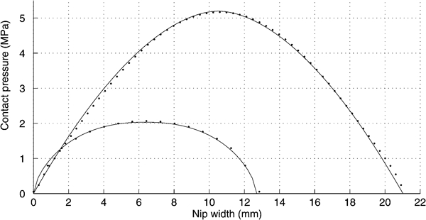
Examples of pressure distributions: larger and sharper is for thin soft rubber layer with high line load; smaller and more blunt is for thick hard rubber layer and low line load; solid line, analytic model; dots, FE calculations

The model behaviour is shown with solid lines and results from FE analysis is shown with dots in Fig. 10. The model behaviour in the two cases shown, is generated with equations (16)–(21).

In addition, the indentation u₁ = 0·39 mm and u₂ = 0·23 mm give the nominal compressive strains ϵ_nom = u/t, ϵ_nom1 = 13% and ϵ_nom2 = 0·9%.

Discussion and conclusions

A model was presented that makes it easy to analyse the influence of parameters in the roller configuration on nip properties. For example, it is easy to make a sensitivity analysis with respect to chosen variables in order to determine the one influencing some aspect of the nip the most.

The results of the fit are satisfactory. The functions could be chosen so that the error between them and the results from FE calculations was held at reasonable levels.

Although the analysis made here relies on a static elastic basis, some dynamic effects concerning stiffness can be taken into account by using dynamic stiffness values for the shear modulus as input to the model. However, the dynamic effects originating from damping in the rubber material, that are influencing the appearance of the pressure distribution and its derivative, in that it is being unsymmetric, is not covered by the model.

Other problems could be treated in a similar way. Solid rubber wheels are used in many applications and could be analysed in the same manner as outlined here, using FE analysis results to determine analytical functions.

References

Batra

: ‘Quasistatic indentation of a rubber-covered roll by a rigid roll’, J. Numer. Meths. Eng. 1981, 17, 1823–1833.

Oden

, Becker

, Lin

: ‘Formulation and finite element analysis of a general class of rolling contact problems with finite elastic deformations’, in ‘Mathematics of finite elements with applications’ , (ed. , Whitemen

J R

, ed); 1985, London, Academic Press.

Parish

: ‘Measurements of pressure distribution between metal and rubber covered rollers’, Br. J. Appl. Phys. , 1958, 9, 158–161.

Parish

: ‘Calculation of the behaviour of rubber-covered pressure rollers’, Br. J. Appl. Phys. , 1961, 12, 333–336.

Austrell

P.-E

: ‘Analytical modelling of hysteresis heating in rolling contact of rubber covered rollers’, Plast. Rubber Compos., 2013, 42, 7, 276–281.

MATLAB Reference Guide, The MathWorks Inc., Natick, MA, USA.

Abaqus Inc., Abaqus user's manual, version 6.5, Providence, RI, USA.

Thomas

, Hoersch

: ‘Stresses due to the pressure of one elastic solid upon another’, Engineering Experiment Station Bulletin no. 212, University of Illinois, Urbana, IL, USA, 1930.