
Abstract
This paper investigated the effects of eight dissolved species concentrations on corrosion of carbon steel in water. Short term electrochemical experimental measurements indicated that the corrosion mechanisms of carbon steel in brackish water are uniform and pitting corrosion. The corrosivity of water is difficult to be defined using single parameter such as the corrosion rate. In this case, Mahalanobis–Taguchi method, as a discriminant analysis approach, is applicable for water corrosivity assessment. Mahalanobis–Taguchi method enables to predict whether a given water sample is acceptably corrosive or not. The preliminary investigation has indicated that Mahalanobis–Taguchi method can serve as a tool for water corrosity assessment.
Keywords
Introduction
Corrosion in aqueous environments is a big issue in oil and gas production. A large part of water applied in the production contains certain amount of soluble, as well as insoluble, species and belongs to brackish water according to the classification of saline water defined by ASTM D1129.1 The brackish water used in the production includes process affected and saline groundwater. Process affected water is generally the combination of waters from the river, precipitation, mine depressurisation and the connate water in miner.2,3 According to water chemistry analysis report,3 the inorganic water chemistry of process water used in oil production include Cl−1, CO2, H2S,  , Ca2+ and Mg2+. Besides, the dissolved O2 and H2S are also known as important contributors to the corrosivity of water. The process affected water is normally O2 saturated, highly conductive and high in organics, microbiological activity and suspended solids. The contaminants in water are strongly affected by the source of the water, mining processes and processes used in production and water treatment. Recent technology advance enables, not yet widely, the use of saline or brackish groundwater in the steam generation process of in situ recovery.4,5 The assessment of water corrosivity is practically important for water management to reduce the cost due to corrosion related failure. Although it is well known that the corrosivity of water is strongly affected by water chemistry and service conditions, the description of the impacts of environmental variables on water corrosivity are normally qualitative.
Some species, such as Cl−, dissolved O2, CO2, H2S,  and
and  , may directly influence the water corrosivity.6 A well known fact is that, within the concentration range of brackish water (<3 wt-%), the corrosivity of water increases monotonically with Cl−1 concentration. Short term immersion tests indicated that the corrosion rate of mild steel in brackish water is proportional to the dissolved O2 concentration.7 Because of corrosion, the dissolved O2 in water may decline, even exhausted, during the transportation in a sealed pipeline.
Some species have an indirect impact on the corrosion. For instance, Ca2+ and Mg2+ alter the water hardness and thereby affect water scaling and clay coagulation. Calcium and magnesium carbonates tend to deposit on steel surface in the corrosion product layer and may thereby slow down the corrosion process. Natural brackish waters generally have pH values ranging from 4·5 to 9. The pH of process affected water depends heavily on industrial processes in use and minerals being processed. Fluctuation in pH may shift various equilibria and thereby change the availability of specific ions. The importance of equilibria is reinforced by a greater role of the calcium–calcium carbonate balance (alkalinity and hardness) of the water than the water salinity on the corrosion of steel. In addition, short term laboratory investigations have indicated that a pH in the range 4-10 is not itself a significant factor in the rate of immersion corrosion8 but indirectly affects corrosion through its effects on the calcium carbonate–carbon dioxide balance. An increase in pH promotes calcite deposit formation that is also a function of temperature and pressure and, to some degree, depends on the concentration of dissolved O2. The formation of carbonate deposit leads to an increase in the thickness of the corrosion product layer. It tends to lower the supply of dissolved O2 to the metal/liquid interface, due to low diffusion rate in the corrosion scale and hence reduce the corrosion rate in ‘hard’ water. However, no direct correlation has been found between water hardness indices and corrosivity of brackish waters.8 The role of carbonate deposit in pitting corrosion is still unknown. The formation of carbonate deposit is reversible, albeit slowly. A decrease in pH slowly dissolves the calcite content in the rust layer, which leads to accelerated corrosion. The impingement of flowing water containing solid suspensions, such as mature fine tailings, may remove the corrosion product layer, bringing about an increase in the corrosion rate.9 The complexity of water corrosivity assessment results largely from the complicated chemical compositions of water, and the different species may react with each other. The various equilibria between various species are affected significantly by temperature and pH. The temperatures in the extraction of oil sands may be as high as 90°C. Elevated temperatures may promote the formation of carbonate deposits.
Bacterial activity is a primary contributor to non-uniform or localised corrosion in brackish water, which depends heavily on water chemistry and service conditions. Only limited investigations have been published in the open literature, up to now, on the corrosion in natural brackish water.2,10 The corrosion behaviour of steel may vary with increasing exposure duration as O2 is depleted in a closed system as a result of corrosion reactions. In anaerobic condition, microbiologically induced corrosion (MIC) may occur in the presence of sulphate reducing bacteria (SRB) that may produce corrosive H2S. The produced H2S in processing is an alternative source of H2S.7,11 H2S is a weak acid. It can raise the corrosion rate with increasing concentration.12 A five year field survey indicated that, with the aid of SRB, the corrosion of mild steel in slightly brackish tropical waters may be more severe than that in sea water.8 Increasing water pH to 9 may slow down the SRB bacterial activity. Since  is the energy source for SRB activity, the MIC may be promoted by increasing concentrations of
  , even if the overall chemical composition of the water does not changed significantly. The solubility of
  decreases when water is supersaturated with calcium carbonate, and this, in turn, would reduce the activity of SRB. Organic matter may serve as nutrients for bacteria, but the direct impact on corrosion is unclear. Generally, MIC is inhibited at high temperatures.
The foregoing has illustrated the complexity of brackish water corrosivity assessment. There are at least three mechanisms in corrosion processes occurring in brackish water, namely, uniform corrosion, pitting corrosion and MIC. Challenges originate mainly from the broad range of brackish water chemistry and the interactive effects of the species present. The processing parameters, such as temperature, flowing velocity and exposure duration, have also important impacts on the corrosion processes. Microbiologically induced corrosion may occur after long term exposure, and it complicates the corrosivity assessment. Corrosion behaviour of steels varies with water chemistry, temperature and exposure duration. The water corrosivity assessment often requires the multivariable analysis. In this paper, an attempt will be made to apply statistical approaches in water corrosivity assessment. As an initial step, only the effects of water chemistry on the short term corrosion behaviour of carbon steel are considered.
Statistical approaches applicable
As described in previous section, multivariable analysis has to be used for water corrosivity assessment because a large amount of variables relating to environmental chemistry, temperature, exposure duration, materials, etc. This paper discusses only the approaches applicable to assess the effects of environmental variables in case the values of those variables can be determined.
When the corrosion is dominated by a well known corrosion mechanism, the corrosivity of water can be assessed by the developing velocity of this kind of corrosion, e.g. the anodic dissolution rates of uniform corrosion, the cracking velocity of stress corrosion cracking and initiation or penetration rate of pits. If the rates for the corrosion development are experimentally determined, the regression analysis can be applied to establish the predictive models on an empirical or half empirical basis. If the corrosion rates are determined in solutions of which the chemical compositions are designed following the orthogonal arrays (OA), according to Taguchi, the relative contribution of individual variable can be evaluated using the range of signal/noise ratio  for individual variable.
  is calculated using the following procedure:13
calculate the signal/noise ratio SN of each test in the OA

 and σ j are the mean and standard deviation of observed values of in the jth experiments listed in OA
calculate the average signal/noise ratio for each level L k of each factor Y i
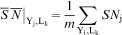
 is the sum of signal/noise ratios SN j when the level of variable Y i, is L k and m is the number of corresponding experiments
calculate the range of signal/noise ratio for each variable
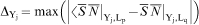
 value is, the more significant role the variable Y i plays in the process being investigated.
The velocity of corrosion development in field is often difficult to be collected. Sometimes, the water corrosivity is difficult to be accurately defined because the dominative failure mechanisms may vary with the environmental and operational parameters. Different parameters are often required to evaluate corrosion development with different mechanisms. The questions to be answered are related to whether corrosion occurring under certain conditions is acceptable or not. In this situation, the discriminant analysis can be done to evaluate the corrosivity of environments. This kind of analysis does not require measurement of corrosion rate. The most commonly used discriminant analysis approach is the Mahalanobis–Taguchi (MT) method.14 This method has been actually applied to the quality control of products in mass manufacture, the recognition of healthcare, fire alarm, handwriting, etc.
The basic approach of MT method is to divide the observations to be analysed into two groups: normal or healthy group and abnormal or unhealthy group in line with the criteria preselected. In the case for water corrosivity assessment, the criteria, such as pits detected, initiation of stress corrosion cracking and occurrence of MIC, may be utilised to separate the water samples or environments into the ‘non-corrosive’ or ‘acceptably corrosive’ group and the ‘unacceptably corrosive’ group. The corrosivity is possibly controlled by n variables such as concentrations of various species in water and/or operational parameters (temperature, pressure, etc.). Each group occupies different subspaces in an n-dimensional space consisting of the n variables. The value of each variable is determined for each test/observation and the Mahalanobis distance (MD) of each test result/observation will calculated. All MDs obtained from the data of the normal group will form the so called Mahalanobis space (MS). This is the most important step of the MT method. The MS established from the data of normal group serves as a database for the corrosivity prediction. According to the MT theory, the MDs determined from the abnormal group must be larger than those of normal group, and thus, they must fall in a so called signal space that is outside of the MS. Hence, the MD can be used as an indicator for corrosivity. Further analysis will be conducted using the concept of signal/noise ratio of each variable to evaluate the significance of this variable.
The discriminant analysis procedure using MT method is as follows:
divide the water samples to be analysed into the normal (acceptably corrosive) and abnormal (unacceptably corrosive) groups according to certain criteria
define the water quality factors or environmental variables Y i, (i = 1, ….n), and y ij is the observed value of Y i in the jth experiment
calculate the MD of the normal group using the following equation
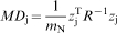


 and σ i are respectively the mean value and the standard deviation of the variable Y i determined from k observations. Then, the distinction data are collected for the water corrosivity assessment. The average of MDs of the normal group is unit so that the MS is also called the unit space. If all variables involved in the analysis are fully uncorrelated or independent, the covariance matrix will be a unit one and the MDs are identical to Euclidean distances. R −1 serves as the database for further corrosivity assessment of unknown water samples
calculate the MDs of individual member in the abnormal group from its environmental variables of abnormal group using equations (4) and (5). In the calculation, R −1 obtained from the data of the normal group will be used
select the variables that have significant impact on the observed corrosivity utilising and the MD of abnormal group and the signal/noise ratio proposed by Taguchi
the database now is ready for the prediction of water corrosivity.
As a discriminant analysis method, the corrosion rate measurement is unnecessary and the MT method provides an answer of ‘pass or fail’ type. If the prediction is proven by experimental or field observations, the data can be used to update the MS to improve its predictive confidence. In this way, the system has a kind of self-learning function and provides greater confidence with data accumulation. The MT method provides a powerful multivariable analysis tool to deal with the kind of engineering problems such as brackish water corrosivity. It has been utilised to assess the corrosivity of fresh water recently.15
Experimental
The test material was hot extruded 1020 steel rod. The specimens with test surface area 1·25 cm2 were mounted in epoxy resin with test surface area. Before electrochemical measurement, the specimens were ground with abrasive paper up to 600 grit, rinsed and dry successively.
The artificial brackish waters were prepared with deionised water regent grade chemicals. Eight dissolved species to be investigated were dissolved O2, pH Cl−,  ,
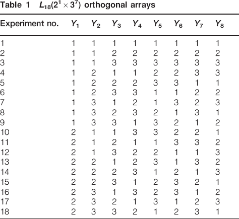
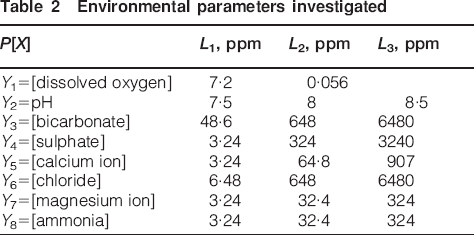
,  , Ca2+, Mg2+ and NH4 +. Eighteen solutions were designed in line with L 18(21×37) OA given in Table 1. The concentrations of individual species listed in Table 2 were selected according to water chemistry analysis reported by Allen.3 The electrochemical measurements were done in the quiescent solutions (the dissolved O2 concentration [O2]≈7·2 ppm) and the deaerated solutions ([dissolved O2]≈0·056 ppm). The deaerated condition was achieved by continuous bubbling of nitrogen into solution for more than 1 h until the open circuit potential of steel electrode was stabilised and the continuous nitrogen bubbling was not stopped before the test was completed.
L 18(21×37) orthogonal arrays
Environmental parameters investigated
Electrochemical measurement included linear polarisation resistance and potentiodynamic curves. To eliminate the impact of solution resistance, the infrared drop compensation provided by Gamry poteniostat was used in the polarisation resistance measurements. The tests were done in a three electrode cell. The potentials reported here were versus standard hydrogen reference electrode. The potential range in potentiodymanic curve measurement was from 0·1 V below the open circuit potential to 1 V. After electrochemical measurement, the test surface was examined to check if pits were formed during electrochemical tests. The uniform corrosion rate is determined from the polarisation resistance R p.
Results
Generally, the carbon steel displays active dissolution behaviour in brackish water, as indicated by the typical polarisation curves (no. 2) in Fig. 1. When  concentration is high and Cl−1 concentration is low, steel is passivated (no. 6). If proper amount of Cl−1 is present, obvious pits can be observed on the specimen surface (no. 9).
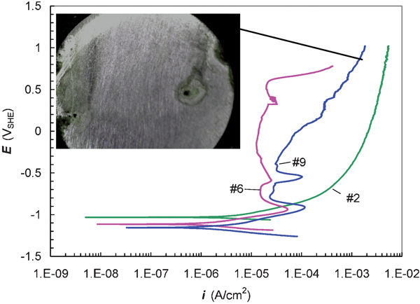
Typical polarisation behaviour and pit morphology
Based on the data of the polarisation resistance R p, the corrosion rates CR were calculated using the following equation
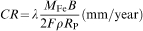

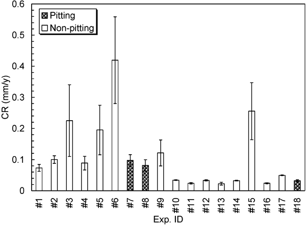
Corrosion rates experimentally determined
Water corrosivity assessment with well defined corrosion rates
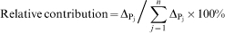
In this section, only uniform corrosion is considered in the corrosivity assessment because the uniform corrosion rates have been experimentally determined. Let x jk = CR jk, where CR jk is the kth measured value of corrosion rate in the jth experiment that is listed in the OA. Then,  and σ j in equation (1) would be the mean and standard deviation of observed corrosion rates in the jth experiments. According to Taguchi method, the signal/noise ratio SN j of each experiment in the OA is given by equation (1). The average signal/noise ratios of corrosion rate corresponding to each level of each variable and the signal/noise ratio range for each variable can be calculated by equations (2) and (3). In the present case, i = 1, …, 8; k = 1 and 2 and m = 6 for dissolved O2 or k = 1, 2 and 3 and m = 9 for dissolved O2 or the rest variables. The relative contribution of individual factor to the corrosivity of water is presented in Fig. 3 with percentage, which is defined as13
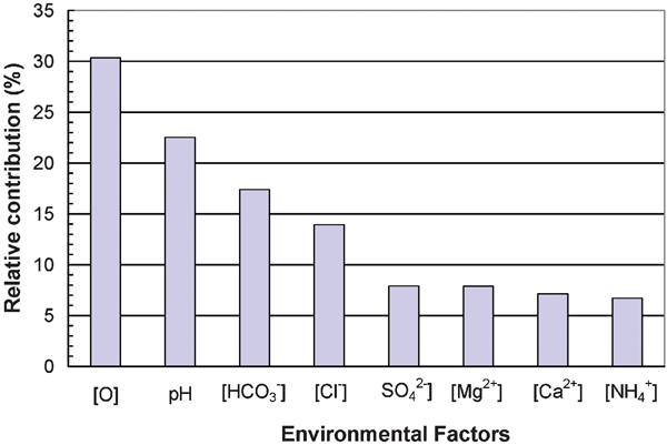
Relative contributions of environmental factors investigated
It can be seen that the dissolved O2 concentration and water pH are two most important environmental factors influencing uniform corrosion in water (>20%). Cl−1 concentration and  are in the second place (in range of 10-20%).
  , Ca2+, Mg2+ and ammonium play minor roles (<10%).
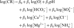
When the corrosion rates and environmental variables are experimentally measured, the correlation between the corrosion rates and the environmental variables can be determined with the multivariable regression method. The function utilised in the regression analysis may be purely empirical or half empirical if certain equations with theoretical background are applied. Since no theoretical formula is applicable to fit the correlation between the uniform corrosion rates and the concentration of corrosive species in water, the following empirical equation is used in the present study to fit the experimental data
Comparison of corrosion rates experimentally observed and predicted by equation (10)
Coefficients in equation (10)

Water corrosivity assessment with discriminant analysis method
Since both uniform and pitting corrosion were observed in the experiments, the data of the normal (acceptably corrosive) group are collected, in the present analysis, according to the following criteria:
the uniform corrosion rate of steel is not higher than 1 mm/year
no pit is detected after electrochemical measurements on test surface by visual observation.
The water samples in which the steel specimen displays a corrosion rate above 1 mm/year or pit is detected after electrochemical measurement are put into the abnormal (unacceptably corrosive) group. As indicated by Fig. 2, the normal group included water samples 1, 2, 4, 7, 10, 11, 12, 13, 14, 16 and 17. The abnormal group contains samples 3, 5, 6, 8, 9, 15 and 18.
With the aid of equation (2), the MDs of the normal group are calculated from the values of environment variables of water samples in the normal group that may be found in Table 1 Tables 1 and 2. The covariance matrix and its inverse are determined form the environmental variables of the normal group, which forms the database for water corrosivity assessment.
After the inverse of covariance matrix was determined by the data of normal group, the MDs of water samples in the abnormal group can be calculated using equation (4). The result is shown in Fig. 5. It can be seen that the MDs of the abnormal group are much larger than those of the normal group.
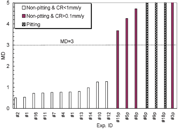
Mahalanobis distances of normal and abnormal groups
The MDs of normal group follows the normal distribution; the MDs of 95·44 of water samples that are acceptably corrosive should fall in the range of  . The mean value of MDs for the normal group
  is unit. Theoretically, the standard deviation of MDs for the normal group is also equal to 1. Hence, MD = 3 is commonly used to separate the normal and abnormal group. The data in Fig. 5 show that the MDs of water samples of abnormal group are >3.
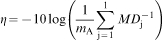
Further calculations using equation (6) were made to determine the signal/noise ratios when one of the environmental factors being investigated has been excluded from analysis. The results are given in Fig. 6. The results show that elimination of any environmental factor investigated from calculation will reduce the signal/noise ratio, i.e. the predictive accuracy. Hence, the eight environmental factors are necessary in water corrosivity assessment.
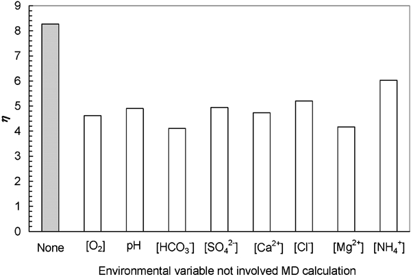
Impacts of environmental variables eliminated from analysis on signal/noise ratios
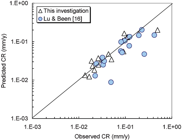
To check applicability of the database established by the present investigation for the water corrosivity assessment, the MDs of the water samples utilised by Lu and Been16 are calculated with equation (4) and depicted in Fig. 7 where the data of abnormal group obtained in the present investigation are also presented for comparison. As indicated in Fig. 7, there are five misjudgements out of 25 water samples that occupy 20% of the total judgements. This analysis indicates that the MT approach may provide a reasonable prediction for the corrosivity of brackish waters. The accuracy of prediction may be further improved if more experimental data are collected and the scale of environmental variables is carefully tuned.
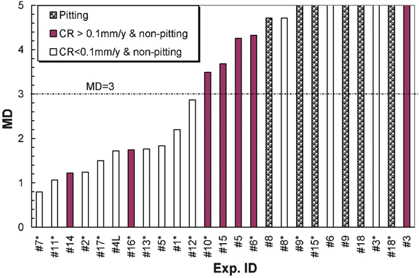
Corrosivity prediction using MDs calculated with database established in this study (data of experiment ID with superscripted asterisk were quoted from Ref. 16)
Finally, it should be pointed out that the conclusions drawn from the discriminant analysis are based on the data that were obtained from short term electrochemical experiments. In principle, this approach is also applicable for analysis of the data obtained from long term experiments, and field observations and the processing parameters, such as temperature, exposure duration and flowing rate, can also be incorporated into the analysis. The discriminant analysis based on the MT method is specifically suitable to predict the likelihood of corrosion related failure resulting from competition of several corrosion mechanisms where the dominative failure mechanisms vary with the environmental and operational conditions. The criteria used to establish the normal group may be reselected according to the requirements from practical engineering. Obviously, the same approach can be used to predict the probability of corrosion related failure of different types, for instance, the initiation of stress corrosion cracking in pipelines, if sufficient data are collected from the field observation.
Summary
This study explored the application of statistical approaches in water corrosivity assessment. If the corrosion rate is well defined, the regression technique enables us to find the correlation between corrosion rate and environmental variables. For the systems where several forms of corrosion may be observed, the regression technique is not suitable because it is often difficult to define single parameter to characterise the different corrosion mechanisms. In this case, the MT method can be used as a tool for water corrosivity assessment. According to the database established using MT method, the judgement can be made for a given environment of which the corrosivity is acceptable or not.