Optimised ore selection from conditionally simulated block models

Abstract

This study considers realistic data for a planned open-pit iron ore mine, but is applicable to any open pit situation. By interpolating drill hole data, grades are generated for a rectangular block model. Each block's grade vector has components for each analyte (chemical element or compound) influencing ore value. Deriving the average (E-type) over many simulations leads to each block being assigned its expected value, and thus underestimates the overall grade variability. Alternatively, interpolation by means of conditional simulation is a method that implements random sampling from an infinite population of solutions. Each conditional simulation has appropriate overall grade variability, but estimating any block's mean and variance requires sampling from multiple conditional simulations. For a block model, an ore/waste selection criterion maximises the expected tonnage at a target grade. This criterion is a linear composite of the grade components, with positive coefficients for the beneficial analyte (Fe) and negative coefficients for the deleterious analytes (such as SiO₂, Al₂O₃ and P). Although conditional simulation often leads to a similar expected grade as kriging for each block, the expected maximum tonnage of ore selectable at a target grade may differ from that obtainable from the E-type solution. We apply the linear composite selection criterion to each of 25 conditional simulations, as well as to the E-type block model. Simulation confirms the distribution of product tonnage to have an expected tonnage that is over 20% greater than that of the E-type model. The method also enables a selection probability to be computed for each block, and thus a probabilistic pit boundary distribution to be identified and used in mine planning. Proposed extensions to this method will consider risk-based scheduling of the multiple selection solutions through minimisation of a derived stress factor and treating the mining process as an iterative system with actual or artificial depletions modelled in line with the mine plan, using the updated state (with new information) to re-evaluate the mine plan for subsequent periods.

Keywords

Ore selection Conditional simulation Kriging Variability

Introduction

One of the key decisions when compiling a mine plan and extraction schedule is ‘what is ore and what is waste?’ (Lane, 1988). Simplistically, ore is that part of a deposit (metal or valuable mineral) that can be profitably extracted, whereas waste is the non-economic part of the mined tonnage that has to be extracted in order to obtain the valuable material. In an iron ore deposit (and many other bulk commodities) the value (or value reduction) of the iron ore depends, to a large extent, on the grade of the contaminants that are extracted together with the revenue generating material.

Production schedules (including stockpile feed and blending requirements) of iron ore, and the associated contaminants, provide mine planners with a means to optimise iron grade, while minimising the variability of contaminant grades (Coombes et al., 2005). Production schedules are generally based on geological and grade models derived through deterministic geostatistical estimation methods (such as kriging). Because kriging is known to underestimate grade variability on a block level, geologists and mine planners have increasingly used conditional simulation to incorporate risk in resource and ore block models (Boyle, 2007, 2009; De-Vitry et al., 2007; Jackson et al., 2003; Jewbali, 2011).

The block model

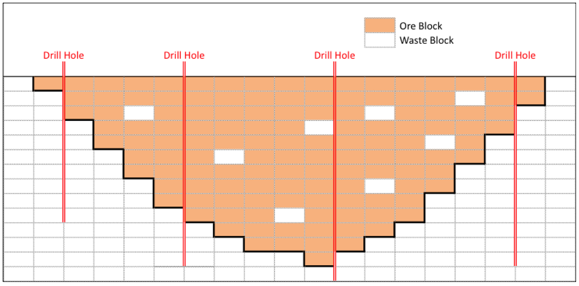
Before proceeding to planning ore selection and sequencing, a rectangular equally spaced block model must be constructed, with grade estimates for each block. For this study, the grades of interest are {Fe, Al₂O₃, SiO₂, P}, but other analytes can be included with no loss of generality. The blocks will measure 30 by 30 m horizontally and 10 m vertically (corresponding to potential mining units). Exploration and subsequent development drilling provide data, generally much coarser than the block interval, which must be interpolated to provide a block model (Fig. 1).

The block model

Spatial interpolation and kriging

We use spatial interpolation to predict their values at each point in the model due to the lack of data to provide a comprehensive set of values for the parameters of interest in a geological setting.

All interpolation algorithms (such as inverse distance squared, splines, radial basis functions, triangulation) estimate value at a given location as a weighted sum of data values at surrounding positions. Interpolation is the estimation of a variable at a location where it was not measured from observed data values at surrounding locations by means of regression. This is usually done by assigning weights to the data values according to the assumption that such weights decrease with increasing separation distance from the location to be interpolated. Geostatistics is an extension of basic interpolation methods, beyond simple linear problems.

Various types of kriging include a number of geostatistical techniques used to interpolate the value of a random field at an unobserved location from observations of its value at nearby locations. Kriging assigns a weighting function based on data using an interpolation algorithm.

Two of the main benefits of using kriging over other interpolation methods are firstly that it helps to compensate for the effects of data clustering by assigning individual points situated within a cluster less weight than isolated data points, thus treating clusters like single points, and secondly that it provides an estimate of the estimation error (kriging variance), together with the estimate of the variable itself

One of the main critiques against kriging however is that ordinary kriging (OK), one of the most reliable local estimation methods, suffers from a problem known as the ‘smoothing effect’. OK estimates do not reproduce the sample histogram because of reduced variance as a consequence of the smoothing effect. In the OK estimation process low values are overestimated and high values underestimated making the estimated histogram narrower than the sample histogram.

Data obtained from drill hole measurement are irregularly and coarsely spaced. Interpolating them to the regular block interval must honour the original data, their autocorrelations across space, and also the cross-correlations between each of the analytes. The standard procedure for this interpolation is kriging (Krige, 1951).

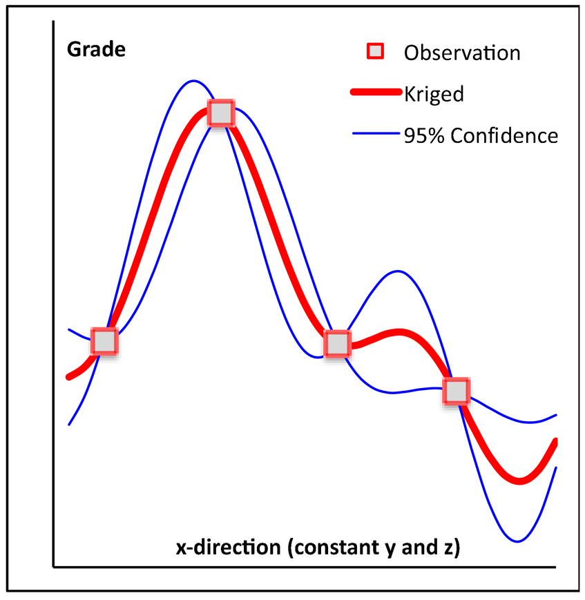
An east-west cross-section of the interpolation (Fig. 2) is simultaneously carried out in all three directions. The thick line shows the kriged interpolation, which is the expected or mean value at each location, while the thin lines show the 95% confidence limits around the mean. The observations shown are data values from drill holes (at equal depth and northing). It should be noted that the 95% confidence range pinches in to zero at the observation points, since each observation is honoured.

Kriged and conditional simulation interpolations

Conditional simulation

Geostatistical simulation is a spatial extension of the concept of Monte Carlo simulation, which reproduces the data histogram as well as honouring the spatial variability of data (usually characterised by an underlying variogram model). If the simulations also honour the individual data points, they are called ‘conditional simulations’ (Journel, 1974; Vann et al., 2002).

Conditional simulation is a geostatistical method that builds many, equiprobable point realisations of mineralisation. Each realisation is different since uncertainty exists for each data point away from the known data points (drill samples).

Conditional simulation is used regularly in the mining industry to communicate information uncertainty and to enhance the understanding of risk. Uncertainties that might lead to potential upside or downside risk are important considerations in determining value in mine design and in decision-making (Coombes et al., 2000). One of the key benefits of conditional simulation compared to kriging is that it removes the smoothing effect witnessed in kriged models.

The kriged interpolation gives the expected grade for each block. For multivariate normal kriging, the kriging estimate is directly the E-type estimate (Olea, 1999, p. 179). However, the actual grade is going to be distributed somewhere around the expected kriged grade. A conditional simulation supplies one possible solution out of an infinite population of solutions, distributed around the kriged solution (Fig. 2). Each conditional simulation has to be consistent, again honouring the autocorrelations and cross-correlations of the source data. For example, considering a single conditional simulation, if one block has a grade much higher than its kriged value, then the neighbouring block will probably not have a grade lower than its kriged value (though that is possible, because of the nugget effect).

A single conditional simulation, being just one member of an infinite population, provides a limited view on the potential variability of data. It is necessary to consider a set of equally likely conditional simulations. For this study, we shall consider a set of 25 conditional simulations, plus the corresponding E-type, for a hypothetical but realistic data set. Twenty-five simulations were used for time and space limitations. Since only grade simulation (and not geology simulation) was done, 25 simulations are expected to be enough to match the variation of grade as defined in the variogram models

During the preparation of data for simulation, UNFOLD functionality of Datamine was used. Chemical variables were transformed to normal scores and normal scores were transformed to minimum/maximum autocorrelation factors (MAFs). MAFs were simulated using the GSLIB sequential Gaussian simulation routine. Point simulation was used. MAFs were then back-transformed to normal scores and normal scores back-transformed to data space. Point simulations were refolded back to dataspace and reblocked to block support. Multivariate dependencies were handled by the use of MAFs.

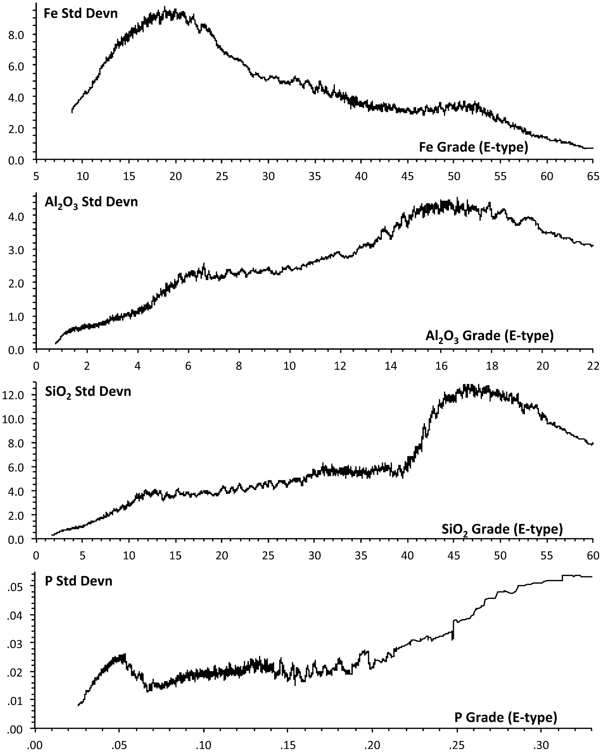
The average of a set of CS realisations (E-type) generally has an expected value similar to the value of the kriged interpolation. The variability of the conditional simulations around the E-type values will vary with location, being zero at the drill hole locations and increasing with distance from the drill holes. Since the drilling interval is likely to be smallest in the richest part of the deposit, the variability will therefore tend to be smaller in the ore zone than in the waste zone. This conclusion is found to be valid with the data set being studied (Fig. 3). The standard deviation between corresponding blocks of the 25 conditional simulations is consistently lower for the blocks high in Fe and lower in the contaminants Al₂O₃, SiO₂ and P.

Standard deviations between the 25 conditional simulations (smoothed over 100 blocks)

The graphs were constructed for each analyte by sequencing the blocks in order of ascending E-type grade for that analyte (Fig. 3). For each block, the standard deviation between the 25 conditional simulations was computed. The graphs show these standard deviations smoothed over 100 blocks, neighbouring in average (E-type) grade.

The correlations between the E-type grades for the four major analytes are shown in Table 1. As is usual, Al₂O₃ and SiO₂ have a strong positive correlation with each other, and both have a strong negative correlation with Fe. In this example, P has a strong correlation with Fe, and negative correlations with Al₂O₃ and SiO₂.

Table 1

Correlations for averaged (E-type) data

	Correlations
Fe	Al₂O₃	SiO₂	P
Fe	1·00	−0·85	−0·95	0·74
Al₂O₃	−0·85	1·00	0·65	−0·65
SiO₂	−0·95	0·65	1·00	−0·72
P	0·74	−0·65	−0·72	1·00

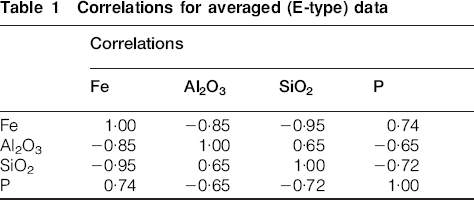
For each conditional simulation, the cross-correlations between the analytes are similar to (but not identical to) the cross-correlations for the E-type values (Table 1).

Ore selection

Estimating the ore tonnage

Selecting the blocks for extraction as ore should ideally have the objective to maximise the net present value. This would be equivalent to including as ore any block whose marginal value exceeded its marginal cost, since both are incurred at or near the time of extraction.

It should be noted that here we are discussing ore selection, not ore sequencing: in some situations, such as gold mining, the net present value can be increased by first mining the higher value blocks, although with iron ore this may not be so relevant since maintaining a consistent product quality is more important. This requires the deliberate inclusion, at each stage of mining, of lower grade blocks that become ore when blended with other higher-grade blocks to form larger parcels with average grades within required specifications.

Because of the need to produce at consistent quality it is very difficult to establish marginal values for lower grade ore that is to be blended. It is therefore more practical to set an objective of maximising the tonnage at a target grade. We shall assume the objective is to extract the maximum tonnage with a target grade of 60·0% Fe and 2·0% Al₂O₃. For the discussion, to facilitate two-dimensional representation, we shall assume that the SiO₂ and P grades are not important, although the models to be considered can readily be extended to include them in the objective. If this is done, the conclusions are not materially changed.

In general current practice, the ore selection is typically applied to the kriged block model using a quadrant cut-off, to select any block whose Fe content exceeds a critical value, provided each contaminant (such as SiO₂, Al₂O₃ and P) is below its critical value. The cut-off values are chosen so as to maximise the tonnage of ore at the target grade.

A difference of opinion

A reviewer of this paper comments: ‘This premise may possibly be true for some operators, but it is not in the case of the multinational corporations that the paper implies. The major iron ore operators typically define ore from waste at the strategic level. The process involves integrating tens and in some case hundreds of deposits and covers many different internal and external scenarios. It is a highly sophisticated optimisation process and involves whole teams of employees using highly sophisticated optimisation engines. It is a vastly more sophisticated process than either the quadrant method that the paper implies is used or the composite method that is suggested.’

The lead author's experience working with the staff of several multinational corporations (and with consultants) is that the quadrant method is applied during the actual mining of the ore body. More sophisticated methods (see below) may have been used in defining the ore body, but within the company such methods do not appear to be clear to the operational staff.

The reviewer also comments: ‘As the author mentions, detailed procedures are not published, that is because they are proprietary. It is a vastly more sophisticated process than either the quadrant method that the paper implies is used or the composite method that the paper suggests.’

It is understandable that the detailed procedures are not published because they are proprietary. However, this means that they are not subject to open peer review. In the lead author's experience, the ore selection process is a black box for the operational staff. The operational objective is generally to maximise ore tonnage at a market grade vector (which changes during operation). I have been unable to find any evidence of any staff being able to express ore value as a function of the grade components {Fe, SiO₂, Al₂O₃, P…}. Given the lack of such a function (which would have to be probabilistic), I remain very sceptical as to the validity of any black box procedures that claim to maximise net present value. For a product such as gold, with a single well-defined product (pure gold) it may well be possible to maximise expected net present value. For iron ore, the product grade is a vector with both Fe and contaminant components (such as Al₂O₃, SiO₂ and P) which must match an agreed market grade. The marketed composition is a negotiated vector, with no assurance that it maximises net present value for the producer. However, given an agreed market grade vector, the operational optimisation is to identify the maximum ore tonnage that can be mined satisfying the required grade. The composite cut-off criterion described here maximises the ore tonnage at a specified grade, whereas the commonly used quadrant criteria do not.

As will be demonstrated, use of quadrant selection and use of kriged interpolation both contribute to underestimating the available ore tonnage extractable at the target grade.

Quadrant and composite selection from the E-type block model

For the quadrant selection method, the cut-off values Fe[cut], Al₂O₃[cut] are chosen with the objective of maximising the tonnage that can be selected with total average grade equal to the target of Fe = 60·0%; Al₂O₃ = 2·0%.

A block is selected as ore if it has grade Fe≥Fe[cut], Al₂O₃≤Al₂O₃[cut].

Applying this criterion to the E-type block model, we find that with Fe[cut] = 49·66% and Al₂O₃[cut] = 2·82%, the ore tonnage at target grade (Fe = 60·0%; Al₂O₃ = 2·0%) is maximised at 92·721 Mt (million tonnes).

However, the quadrant criteria can be shown to underestimate the available tonnage, because the criteria exclude blocks that, if combined, would then satisfy the same cut-off criteria. A further illogicality arises when the quadrant approach is applied to a prospect with multiple pits that have systematically different composition. We then find that applying a different set of cut-off values to each pit increases the ore tonnage available at the target grade. This is clearly illogical, because it implies that an ore block that would be selected as ore from one pit would be rejected as waste if it occurred in the other pit. Both these illogicalities indicate that the quadrant cut-off method is not optimal. Nonetheless, we have observed, over the past two decades in several companies, on many prospects, that quadrant cut-off criteria are used in practice. Although detailed procedures are not commonly published, Boyle (2009, p. 47) confirms the use of the quadrant cut-off criteria (‘For this study, three chemical parameters are used to define high-grade ore in block classification: Al₂O₃<5 per cent, Fe>57 per cent, and SiO₂<10 per cent’).

Instead of applying a set of quadrant cut-off criteria, it is preferable to use a single composite cut-off criterion, accepting as ore any blocks that satisfy the single criterion: (1) The constants K_Al and X[cut] are chosen so as to maximise the ore tonnage averaging the target grade. It can be shown that the composite grade cut-off criterion will always give an ore tonnage at least as large, and commonly up to 10% larger, than does the quadrant cut-off method (Everett, 2011).

Choosing the constants K_Al and X[cut] so as maximise the ore tonnage at the target grade can readily be done by a simple iterative hill-climbing search, since the objective function (tonnage selected) behaves smoothly in the search area defined by K_Al and X[cut]. The method can be readily extended to include coefficients for other analytes of interest.

Naturally, both ore selection methods depend upon there being a feasible solution: if the target grade is infeasible, specifying an unattainable grade combination, then there will be zero ore identifiable by any method.

Having identified the maximum ore tonnage at target grade, the problem remains to extract it in a feasible sequence so as to produce continuously at target grade with minimum need to stockpile and reclaim. This issue is considered in the later section of this paper under ore sequencing, and is discussed by Everett (2011).

Applying the composite criterion to the E-type block model, we find that solving the algorithm with parameters K_Al = 7·5418 and X[cut] = 35·947, maximises the ore tonnage at 95·553 Mt. Thus, in this example, the composite ore select criterion gives 3·1% more ore than does the quadrant selection method.

Blocks in area A are selected as ore by the quadrant method, but not by the composite method (Fig. 4). Blocks in areas B and C are selected as ore by the composite method, but not by the quadrant method. The tonnage in areas B and C will always be at least as great, and usually greater, than the tonnage in area A. Therefore, the composite criterion will always select at least as much, and generally more, ore than is selected by the quadrant criterion.

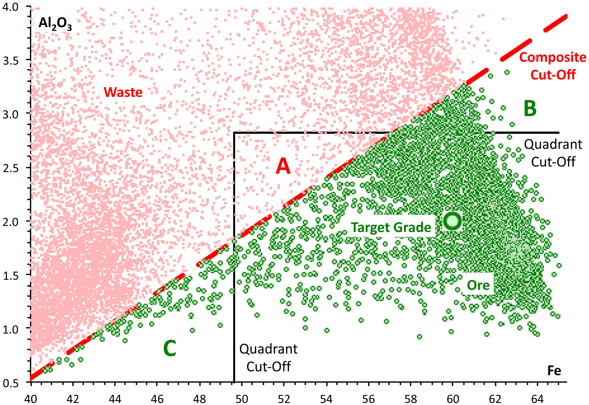
Composite and quadrant cut-off procedures

Composite selection from the conditional simulation block models

The composite selection procedure was next applied to each of the 25 conditional simulation block models, so as to maximise the ore tonnage at the target grade of Fe = 60·0; Al₂O₃ = 2·0.

The ore tonnage was consistently greater for every one of the conditional simulations than it was for the E-type block model (Fig. 5). The average ore tonnage for the conditional simulations was 116·61 Mt, with a standard deviation of 1·72 Mt. The average of 116·61 Mt for the conditional simulations is 22% greater than the 95·55 Mt yielded by the E-type solution. Again, this systematic difference occurs even though the E-type grade for each block is the average of the 25 conditional simulation grades for that block.

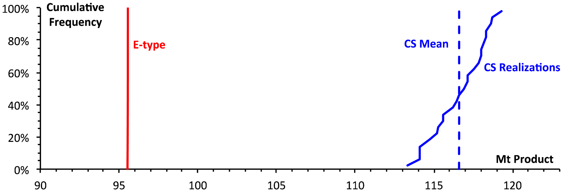
Conditional simulations give higher ore tonnage

There are two cumulative reasons for the conditional simulations giving greater ore tonnage than does the averaged (E-type) model. If we consider the cut-off grade for the E-type model (which we can assume is above the median grade) then a conditional simulation, having a greater variance around the same mean, will have more ore above the E-type cut-off. Because of the longer upper tail derived from the conditional simulations, the ore selected from conditional simulations will have a higher grade than the ore selected from the E-type model, if we apply the E-type cut-off value. So to get the ore grade back to target, the cut-off grade for the conditional simulation can be reduced, below the cut-off for the E-type model. This will further increase the ore tonnage for the conditional simulation.

We can draw the general conclusion that the E-type model systematically underestimates the ore tonnage since reality should correspond to one of the infinite possible conditional simulations (Fig. 5). For this realistic case study, the average model's underestimation of ore tonnage is a considerable 22% below the real average ore tonnage of the conditional simulations.

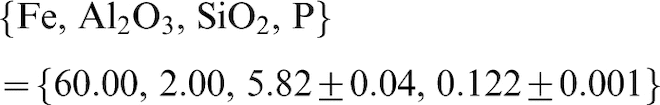
For the ore selected from each of the 25 conditional simulations, the product grade was: As explained earlier, for simplicity and representation in two dimensions, the target grade in each case was set for Fe and Al₂O₃ only, with SiO₂ and P being allowed to find their own levels for this example study.

Although the composite cut-off function coefficients and the composite cut-off values (K_Al and X[cut]) differed slightly between the 25 individual conditional simulations, they differed consistently from the E-type cut-off, (even though the E-type grade for each block is the average of the 25 conditional simulations; Fig. 6). Every one of the conditional simulation composite cut-off functions had a markedly steeper slope of Al₂O₃ against Fe than did the cut-off function for the average (E-type) model.

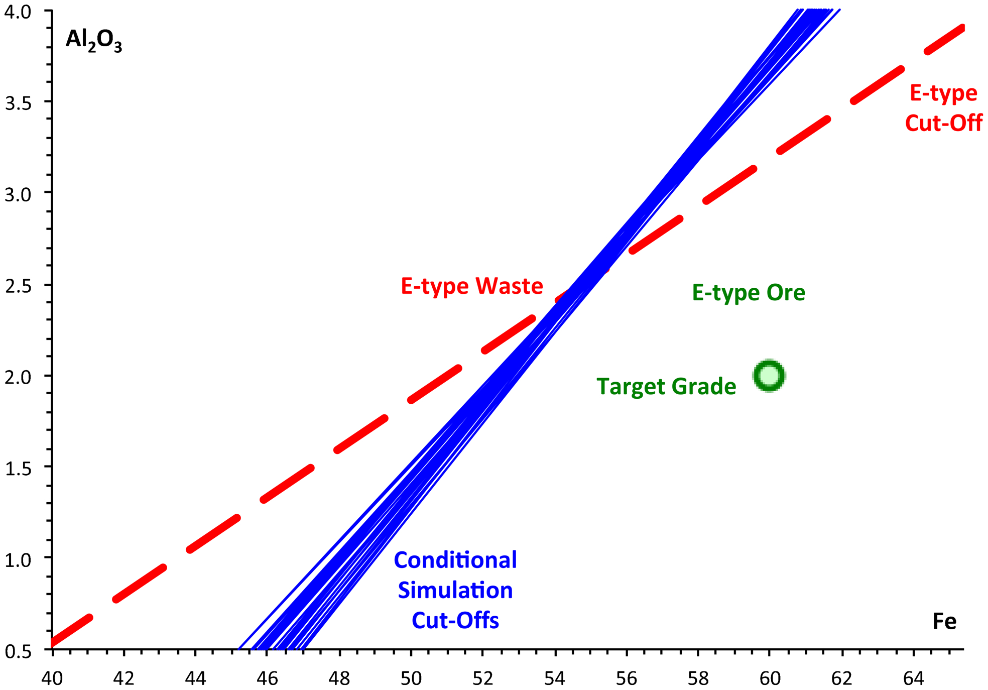
E-type and conditional simulation composite cut-off grades

Ore selection probability

Not all blocks selected as ore from the E-type data set were also selected from the conditional simulations, and similarly some of the blocks selected from the conditional simulations were not included in the E-type solution. However there was a strong relation between the selection sets: Fig. 7 plots the proportion of the 25 conditional simulations selecting a block as ore against the block's composite score for the E-type data set. (For clarity, the plot is smoothed over 100 blocks with consecutive E-type composite scores.) Any block with a composite score exceeding the cut-off value of 35·947 was selected as ore in the E-type data set. Blocks with high E-type composite score were selected by most of the conditional simulation solutions, and blocks with low E-type composite score were rejected by most of the conditional simulation solutions. As E-type scores increase in the region of the cut-off score, there is a rapid increase in selection probability.

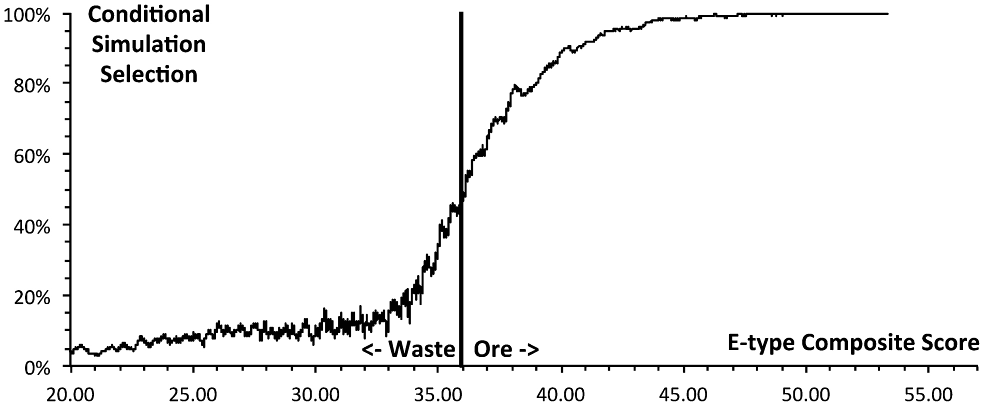
Proportion of conditional simulations selecting as ore (smoothed over 100 blocks)

The selection zone for the E-type data set differed consistently from the selection zones for the conditional simulations (Fig. 6). The implications of this selection difference are made more explicit in Fig. 8. In this figure it should be recognised that the plotted points for each block correspond to the E-type grade of that block. This grade is the average of the 25 conditional simulation grades for the block, but each of the 25 conditional simulation grades will be scattered around this grade value.

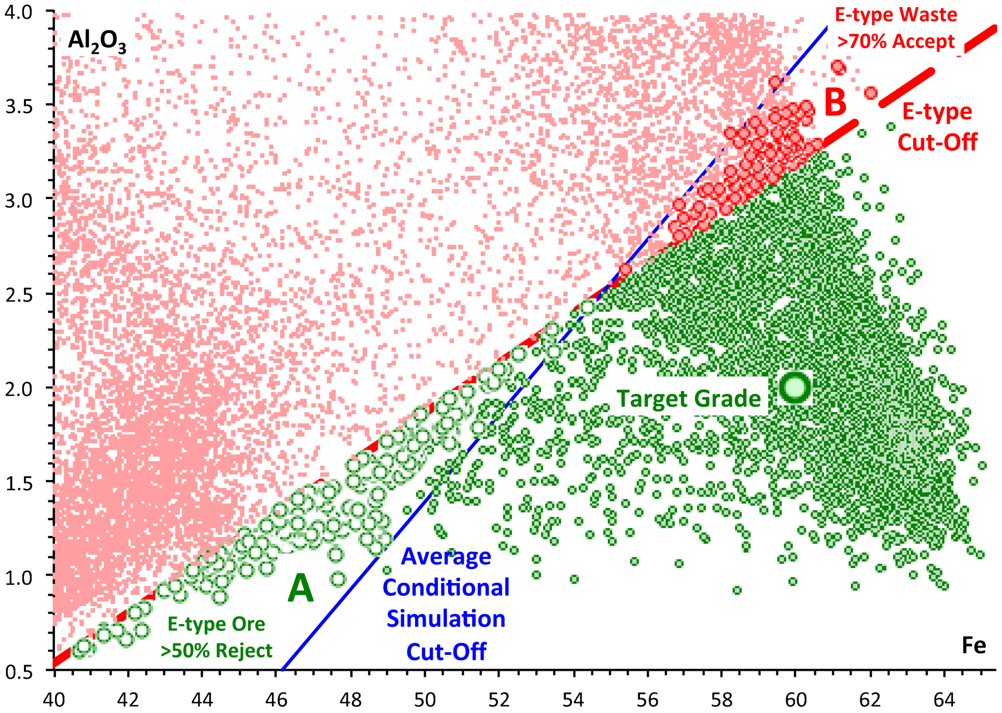
E-type and conditional simulation ore selection (% accept/reject refers to conditional simulations)

The conditional simulation cut-offs have a steeper gradient than the E-type cut-off. Consequently blocks in the region marked A on the plot, with low Fe and Al₂O₃ grades, are likely to be rejected as waste by the conditional simulations even though they were accepted as ore in the E-type model. E-type ore blocks with a greater than 50% conditional simulation rejection rate are shown as larger open circles. Conversely, blocks in region B of the plot, with high Fe and Al₂O₃ grades, are likely to be accepted as ore by the conditional simulations even though they were rejected as waste in the E-type model. E-type waste blocks with a greater than 50% conditional simulation acceptance rate are shown as larger filled circles.

Sequencing the mine plan

Ore sequencing is generally applied to the ore blocks identified from the E-type block model. Let us first consider this situation, and then expand the discussion to consider ore selection taking the conditional simulations into account. The ore blocks need to be sequenced for mining in an order that is feasible, safe and technically efficient, while producing a stream of ore that is consistently close to target grade. Feasibility requires that no ore block can be extracted before an overlying ore block. Safety requires that during the mining process no cliff face (bench height) should ever exceed a safe height (perhaps 10 m). Technical efficiency requires that successive ore blocks should be mined without excessive equipment movement. If multiple pits or mining locations are operated simultaneously, then it will also be necessary to balance the rates of production from these multiple sources, so that equipment is not unnecessarily forced to be idle.

Available block list (ABL) and trimmed block list (TBL)

The set of all the accessible live ore blocks that are available for immediate mining, without first having to remove any other ore blocks, is referred to as the ABL. The complete ABL may well have a combined grade that is very different from the target grade. It may also be of a total tonnage much greater than we wish to consider for a single planning period (such as one week), and may involve too much equipment movement to be acceptable within the planning period. Accordingly, it is necessary to extract a trimmed or reduced subset of the ABL. This TBL must satisfy the objectives and constraints for a single planning period (Everett and Rimes, 2010).

Having mined the TBL, removing its blocks from the block model generates a new ABL. This comprises the residue of the previous ABL, plus the ore blocks that have now been exposed. Again a subset TBL is selected from the new ABL, and the planning process repeated through the life of mine. It should be recognised that although a forward plan is thus created for the life of mine, it will need to be continually updated as blocks are mined and assayed and the revised data used to modify the kriged and conditionally simulated block models for the remaining prospect.

Initiating the mine plan sequence

The mining sequence needs to be initiated with a subset of the first available block list. Given the knowledge obtained from the conditional simulations, we can now select an augmented ABL not only from the E-type ore blocks, but also from the E-type waste blocks that have a high probability of being selected by the conditional simulations.

It should be kept in mind that the actual grades to be discovered in mining would closely correspond to one of the infinite population of possible conditional simulations. To the extent that the conditional simulations have been found to behave consistently differently from the E-type model, it is appropriate to include their information in the choice of the initial mining location.

From the case study data, the augmented first ABL is mapped (Fig. 9). Four categories of blocks are identified:

(i)

category 1: E-type ore blocks also selected as ore by more than 50% of the conditional simulations

(ii)

category 2: E-type ore blocks rejected as waste by more than 50% of the conditional simulations

(iii)

category 3: E-type waste blocks selected as ore by more than 70% of the conditional simulations

(iv)

category 4: E-type waste blocks selected as ore by between 50% and 70% of the conditional simulations.

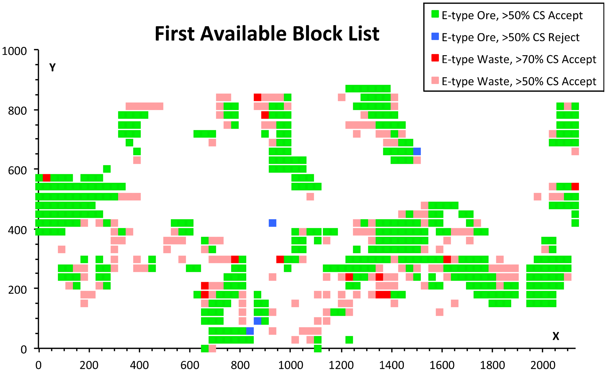
The augmented first available block list (ABL)

In deciding where to initiate the mining, the ABL is reduced to a TBL by the criteria discussed above (meeting grade in the short-term, moderate equipment movement and balancing production between multiple pits or locations). To these criteria we can now add criteria derived from the conditional simulations. The initial mining should preferably use Category 1 blocks, where both the E-type and conditional simulation models indicate ore. If the initial TBL has to be extended beyond the Category 1 blocks, then Category 3 may well be preferable to Category 2.

Continuing the sequence

Having selected the first TBL, the next ABL can be similarly identified from the remaining blocks, the next TBL selected as a subset, and so on iteratively. In initial planning of the mining operation, no further information is obtained at each ABL/TBL step, so the iterative decision-making has to be carried out using the initial E-type and conditional simulation block models. However, in operating the mine, each TBL extracted will provide more information enabling the block models to be updated. With accurate record keeping and adequate data processing, the block model then becomes an evolving information system.

Progressive mining – iteration and adaptation

Exploratory drilling, sampling and lab elemental assaying is usually seen as the main means of gathering information on a deposit or defined mineral resource. However, results from mining and from sampling mined ore provide invaluable additional information that should be systematically recorded and reintroduced into the modelling and estimation sequence. By taking account of the new information obtained from mining (and to some extent from simulations of mining) we can update the resource model for realised and for forecast grades and thus reduce the variability of inferred information by replacing simulated data points with actual data.

Conclusions

Analysis of the iron ore case study has supported and confirmed the benefits of:

Using a composite cut-off grade metric for determining the maximum ore tonnage and allowing for the impact of deleterious analytes.

Using conditional simulations instead of a kriged or E-type model as the basis for ore definition.

After imposing a target average grade of 60% for Fe and 2·0% for Al₂O₃ to the E-type resource model, applying the quadrant cut-off method indicated that an Fe cut-off of 49·66% and Al₂O₃ cut-off of 2·82% would lead to a maximum ore tonnage of 92·7 Mt.

Applying a composite cut-off grade criterion to the E-type model increased the maximum ore tonnage at target grade by 3·1%, to 95·6 Mt. With the composite cut-off function, a linear composite of grade is used as the cut-off value, so that blocks are accepted as ore if X = Fe–7·542Al₂O₃>35·95.

Using the composite cut-off criterion on conditional simulations instead of the E-type model increased the maximum ore tonnage on average by a further 22%, to 116·6±1·7 Mt. The composite cut-off function for the conditional simulations differed consistently from the composite cut-off function for the E-type model. With the conditional simulations, blocks were accepted as ore if X = Fe–(4·32±0·22) and Al₂O₃>44·00±0·62.

A further benefit of using conditional simulation rather than kriging or E-type averages to define models is that a probability can be associated with the likelihood of a block being selected as ore or waste. Some blocks assigned as ore by the E-type model showed a low likelihood of selection when variability was taken into account by conditional simulation. Conversely, some blocks identified as waste by the E-type model actually had a high likelihood of being ore when using the conditional simulations. These findings provide additional useful information in guiding the priority for mining blocks during production scheduling.

Further research and case studies may include the simulation of mining and subsequent inclusion of new information and re-modelling (via conditional simulation) to lead to an iterative, adaptive system that continues to provide the best possible guidance in decision making given available information.

Footnotes

Acknowledgement

The authors wish to thank the Australasian Institute of Mining and Metallurgy (AusIMM) for permission to publish this manuscript, which was originally presented at the AusIMM Iron Ore Conference in Perth in August 2013.

References

Boyle

. 2007. Comparison of multivariate conditional simulation methods at the Yandicoogina Iron Ore Deposit, Proceedings Iron Ore 2007, 57–66, Melbourne, The Australasian Institute of Mining and Metallurgy.

Boyle

. 2009. Multivariate conditional simulation of iron ore deposits – advantages over models made using ordinary kriging, Proceedings Iron Ore 2009, 43–50, Melbourne, The Australasian Institute of Mining and Metallurgy.

Coombes

, Standing

, Lacourt Rodrigues

and Quieroz

. 2005, Exposing uncertainty in schedules for proactive stockpile planning, Proceedings, Iron Ore 2005, 263–266, Melbourne, The Australasian Institute of Mining and Metallurgy.

Coombes

, Thomas

, Glacken

and Snowden

. 2000. Conditional simulation – which method for mining?, Geostats 2000, Cape Town, South Africa, April 2000, 1–15, Document Transformation Technologies – Printed in South Africa.

De-Vitry

, Vann

and Arvidson

. 2007. A guide to selecting the optimal method of resource estimation for multivariate iron ore deposits, Proceedings Iron Ore 2007, 67–77, Melbourne, The Australasian Institute of Mining and Metallurgy.

Everett

. 2011. Ore selection and sequencing, Appl. Earth Sci., 120, (3), 130–136.

Everett

and Rimes

. 2010, A mine-planning model to satisfy long-term grade targets, Appl. Earth Sci., 119, (3), 183–187.

Jackson

, Fredericksen

, Steward

, Vann

, Burke

, Dugdale

and Bertoli

. 2003. Geological and grade risk at the Golden Gift and Magdala Gold Deposits Stawell, Victoria, Australia, Proc. 5th Int. Min. Geol. Conf., 1–8, Bendigo, Victoria, The Australasian Institute of Mining and Metallurgy

Jewbali

. 2011. Multivariate block co-simulation of an iron ore deposit, Proc. 35th APCOM Symp., 157–166, Melbourne, The Australasian Institute of Mining and Metallurgy.

10.

Journel

. 1974. Geostatistics for the conditional simulation of ore bodies, Econ. Geol., 69, (5), 673–688.

11.

Krige

. 1951. A statistical approach to some mine valuations and allied problems at the Witwatersrand, Master's dissertation, the University of Witwatersrand, South Africa.

12.

Lane

. 1988. The economic definition of ore: cut-off grades in theory and practice, London, Mining Journal Books.

13.

Olea

. 1999. Geostatistics for engineers and earth scientists, Boston, Kluwer Academic Publishers.

14.

Vann

, Bertoli

and Jackson

. 2002. An overview of geostatistical simulation for quantifying risk, Proceedings Geostatistical Association of Australia Symposium on ‘Quantifying risk and error’, Perth, Australia, March, Geostatistical Association of Australia, 1–12.