
Abstract
The Central Jordan Uranium project has made use of modern technology in all aspects of the conceptual studies undertaken on this mineralisation to date. Sampling was part of that effort, with special focus on sample preparation and ore heterogeneity. The practical applications of sampling theory and its experimental implementation in the project are described in this paper, including discussion of the main steps required and the benefits of using this approach to the project.
Introduction
In order to ensure the high quality of the samples, the project team has optimised the sampling protocol using methods of theory of sampling (TOS). In particular, emphasis was placed on using heterogeneity tests, which are the most advanced and recently developed techniques that allow the quantitative estimation of liberation factors and the determination of the sampling constants used for estimation of fundamental sampling error (FSE) values. The general issues when studying a project of this kind include:
Determining whether the sample preparation protocols in use are adequate and unbiased and precisely report the assayed sample grades. Evaluating existing protocols and optimising their precision and cost. Gaining insights as to whether dangers exist in sampling the prospective ore and what steps are eventually required to avert them. Determining which combination of area, element and mineralisation type poses the toughest sampling challenge, so as to focus the study on that worst case. Characterising/predicting the response of the sample material above liberation size (general case of regular samples) and eventually, the very different response to be expected below liberation size (i.e. when the ore is completely liberated, meaning it was pulverised to so fine that the individual fragments of the material to sample are either pure gangue or pure mineral). This characterisation implies calibrating the parameters of a variance prediction model known as Gy's formula (i.e. the variance of the FSE). Applying the resulting model formally to calculate sampling variances and representing the current preparation protocols using sampling nomograms, i.e. graphic representations allowing us not only to evaluate the protocols but also to optimally modify them.
To that effect, the following steps need to be undertaken:
Because the models used are calibrated to experimental reality and the parameters thus estimated have physical counterparts, the exercise also allows for an increased understanding of the mineralisation and its mineralogy. Once the model is fully calibrated and available, any variance calculation can take place.
Theory of model
Modern sampling theory, developed by Pierre Gy in the 1950s (Gy 1979) and continued by Francois-Bongarcon (1998) in the 90s, provides a formula, best known as ‘Gy's formula’ to predict the relative variance of a sample (i.e. characterise its reproducibility) as a function of the macroscopic properties of the ore, the comminution size d (i.e. P95 nominal size), and the sample and lot masses MS and ML as

 the liberation factor is usually modelled as
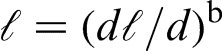
 , the mineral liberation size, relates directly to the size of the coarsest grains of mineral or metal, and b is an exponent that must normally also be experimentally calibrated. When the liberation size is not directly interpretable, the sampling constant
 is calibrated as a whole, along with exponent alpha = 3 − b.
Fig. 1 shows a hypothetical, schematic calibrated model: based on experimental data points (sampling variance at various comminution sizes); this model is fitted to the correspondence between the experimental relative sampling variance per gramme and per parts per million of U element and the comminution size. The log–log graph has two linear parts: one of slope 3 for small sizes, then a portion with a positive slope lower than 3. The abscissa of the separation point between these two portions is the mineral liberation size (i.e. the size at which ore material should be comminuted to in order to liberate most of the mineral grains responsible for the sample variance).
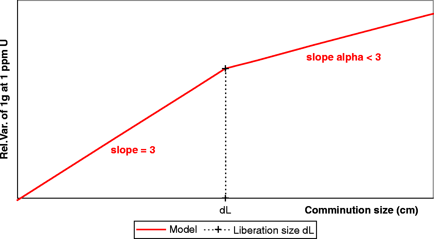
Gy's formula generic calibration graph
Model experimental calibration
Alpha determination
Exponent alpha in equation (3) was first determined using an experiment consisting of calculating single stage experimental sampling variances from a series of samples at various comminution sizes, namely pulps passing 66.6, 2, 0.475 and 88 μm. Analytical error variances were previously modelled as described in Francois-Bongarcon (1998) and were subtracted. The following model was experimentally fitted by asymptotic analysis to pairs of pulp duplicates
†

The formalism of equation (1) was used to adjust all resulting experimental points so that they could be plotted on a graph, similar to Fig. 1 for the same unitary masses and U grades.
Liberation size and mineralogy
It is important to precisely determine the parameter
 or ‘liberation size’ in Fig. 1 (where the two straight lines join) as the variance formula is different above and below this size and a grossly inadequate estimation of this parameter will bias the variance determinations by the use of the wrong formula variant.
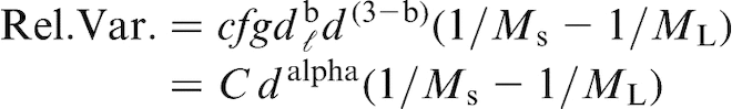
Below liberation size, equation (1) simplifies to

 are absent.
In fact, equation (4) depends only on the mineralogy (via parameter ‘c’, as f and g are just practical convenience variables relating to the geometry of the fragments). This parameter the same for all U deposits with identical grades and same mineralogies. Once alpha (i.e. the slope the rightmost line segment on Fig. 1) is estimated, then the liberation size
Experimental (from the variance of sample crushed so finely that minerals are is fully liberated). Theoretical (from the mineralogy, which allows to calculate parameter ‘c’, which depends only on the densities of the gangue and pure mineral and on the concentration at which the formula is considered). can be fixed by the vertical position of the leftmost segment of slope 3. Two methods can help position that line:
In this case, probably as the result of experimental as well as analytical imperfections, experimental data from a variety of pulverised materials were at odds with the mineralogy that consisted mostly of carnotite, i.e. the green line on Fig. 2. This is not usual, but it can be related to the degree to which the data used, especially the routine pulp duplicate assays, had been ‘cleaned up’, before being released by the laboratory, as exemplified by the re-assaying of odd results, that is visible in Fig. 2. After careful considerations, including sensitivity to the handling of outlying results
‡
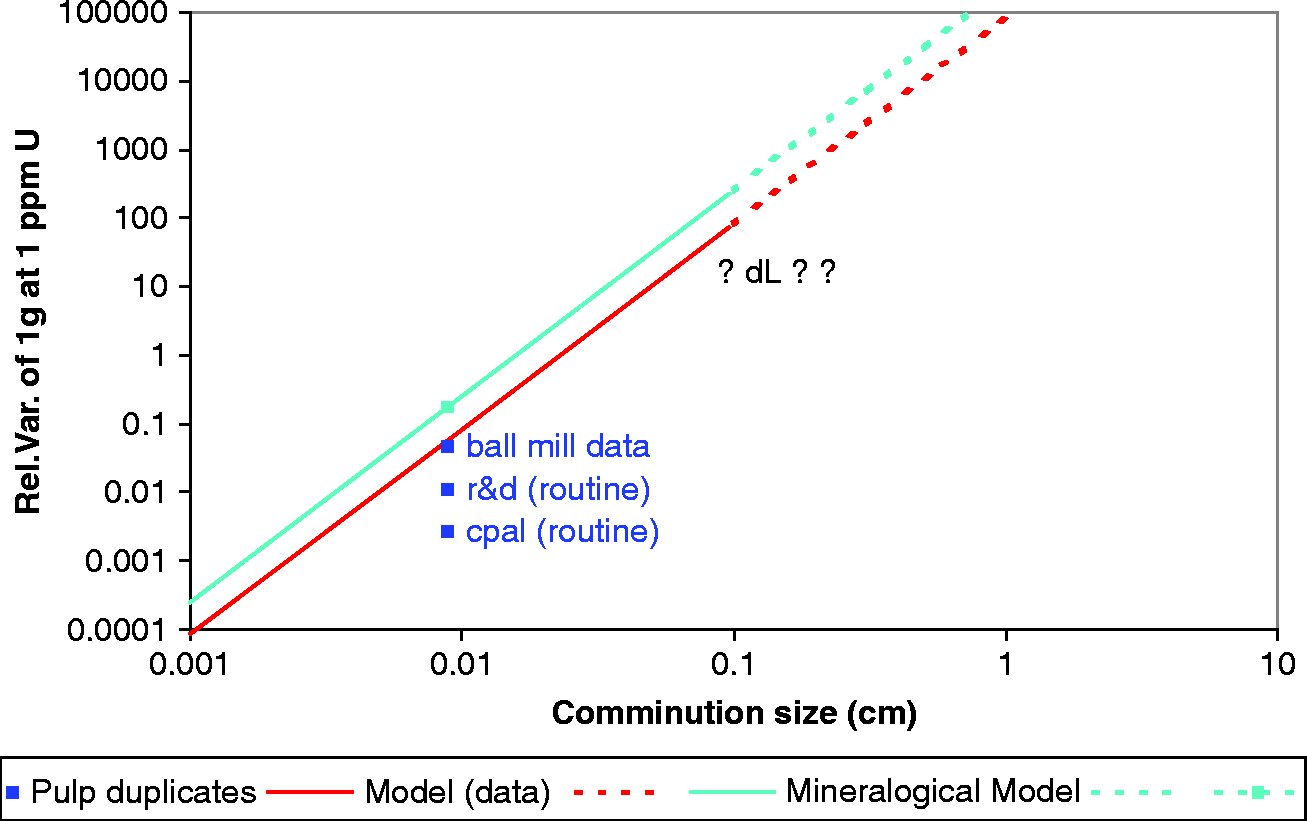
, the model for pure carnotite was adopted, and alpha values were estimated, resulting in the final model represented in Fig. 3, for a value of alpha equal to 1.25 and a liberation size of 523 μm. This corresponds numerically to the following variance prediction formulae
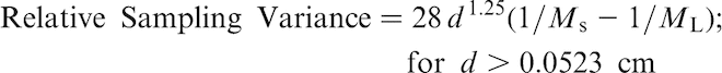
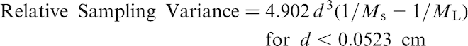
Gy's formula calibration mineralogical options
Gy's formula calibration
Sampling nomograms and protocol optimisation
All sample preparation protocols for both channel and core samples were evaluated using these heterogeneity results. All current types of samples follow the same preparation protocol:
Drying. Jaw-crushing. Disk milling of the entire crushed sample. Splitting to 300–350 g. Pulverising in a ball mill to a nominal size of at least 80% passing 63 μm (P95 ≅ 110 μm). In reality, the P95 size is better, as it was measured to average 88 μm for the calibration experiment.
Since splitting core is not a sampling operation, it incurs no variance if present. Channel samples are not currently split before being processed meaning that therefore they do not have a primary sampling variance. Ways of reducing the sample mass are yet to be examined. Should reverse circulation (RC) drilling be used and a primary sample be split from the cyclone, a new evaluation would be required for this primary sampling step using equation (5).
A particularly useful way of visualising a preparation protocol is the sampling nomogram. It is a log–log graph on which the successive total variance components incurred at the corresponding steps of the preparation (alternated comminution and sampling operations) are represented as a sawtooth path (sampling operations as segments on inclined lines of slope − 1 representing the various comminution sizes, and comminution steps as vertical segments jumping from one line to a lower one). The above protocol produced the nomogram of Fig. 4.
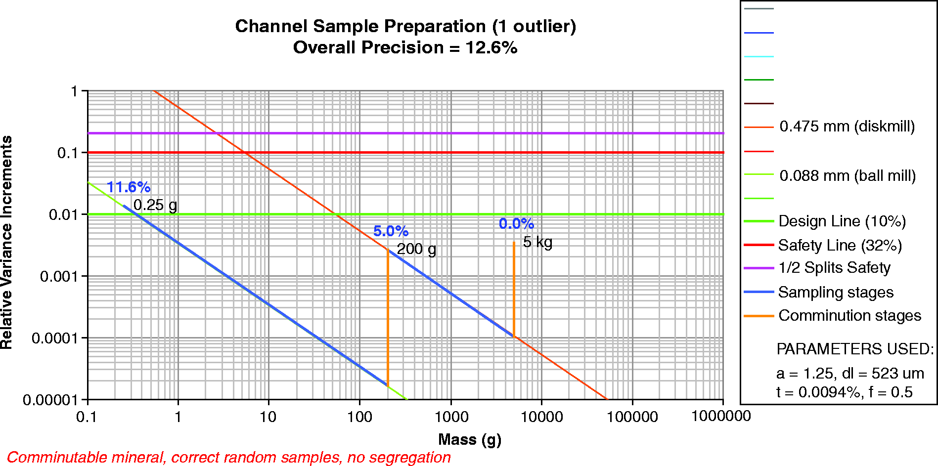
Central Jordan Uranium project
On this graph, special attention is paid to a number of features:
All steps must imperatively be below the red ‘safety’ line, above which sampling is so insufficient (i.e. unrepresentative) that a very unfavourable series of problems occur that are conducive to systematic under-reporting of sample grades. Ideally, and if possible, all steps should be below the much desired ‘design’ line (corresponding roughly to a precision of 10% or better for each sampling step). All saw-teeth should be on approximately the same horizontal level, i.e. the protocol should be balanced (indeed, a tooth higher than the other ones unambiguously characterises the weakest step of the chain, responsible for most of the total variance).
As can be seen in Fig. 4, the original protocol was almost perfectly balanced and satisfactory and no particular problem was detected.
Discussion and conclusions
In this particular case, the greatest challenge was finding the most plausible estimate of the liberation size. Two difficulties were encountered:
Outliers: Because of imperfect assaying and/or experiment implementation, some of the data were not compatible with other data. The choice of the extremes to be treated as such and eliminated led to significant variations in the end results. Most of these issues were resolved by simply keeping the resulting parameters (e.g. liberation size) within plausible ranges of values. Yet, for a couple, there was no way to know for sure and the most conservative calibration was adopted as safer to use. Pulp samples: pairs of duplicates from various sets of pulverised material gave experimental variances that were too small for the liberation size to be within a plausible range (assuming liberation sizes of 1 mm or more were not). In addition the most likely mineral assembly (carnotite type), given its U content and density, indicated calculated liberated variances that were much higher (see Fig. 2) and corresponding to lower, more plausible liberation sizes in the 200–550 μm range (depending on the chase for outliers in the data set used to estimate parameter alpha).
As a result, two decisions were made:
The experimental pulverised duplicates were deemed to be faulty, i.e. likely ‘cleaned up’ by the removal of large differences, thus masking the true variability of the pulps. As such, a decision was made to rely on the theoretical variance of pure carnotite. This first decision made, two equally probable outlier elimination alternatives still produced two sets of results, both with acceptable liberation size estimates (257 and 523 μm respectively). The first result was more likely, both in terms of liberation size and outlier choices, but was less conservative for the prediction of variances and the optimisation of current and future. As such, a temporary choice was made to retain the second set, with a later decision to be made between the two cases on the basis of new data.
To understand why these decisions were important to make as carefully as possible, consider hypothetical Fig. 5, which shows what happens if a model is retained that has a grossly wrong liberation size (i.e. the wrong abscissa for the breaking points between the two linear segments of the model). Authors will assume that the solid lines are the right choice and the dotted lines the wrong one, and will keep in mind the vertical variance scale is logarithmic, so that appreciable variance differences on the graph are in fact wrong by orders of magnitude.
In conclusion, the study is still left open with some ambiguities to be resolved experimentally when more data are collected § , but given that existing protocols were found to be satisfactory even when evaluated using the more conservative of the two models, the study was conclusive anyway. This situation, however, is very rare in practice, and, usually, existing protocols do need to be optimised, making all the considerations above absolutely paramount.
Acknowledgements
His excellency Dr Khaled Toukan, Head of the Jordan Atomic Energy Commission is thankfully acknowledged here for his encouragement to publish the work performed on that project, and his entire technical team, and more particularly Dr Samer Kahook, for making this work useful and stimulating. Several reviewers are also acknowledged for the time they kindly took to help improve this paper with extremely valuable and detailed comments.
Footnotes
* See Gy (![]() ) for more details on these constants, that define intrinsic heterogeneity: d being the nominal fragment size; f being the factor accounting for the shape of the fragment; g being the granulometric factor accounting for the size differences between the fragments; c being the mineralogical factor accounting for maximum heterogeneity condition and l being the liberation factor accounting for the degree of the liberation in the sample.
) for more details on these constants, that define intrinsic heterogeneity: d being the nominal fragment size; f being the factor accounting for the shape of the fragment; g being the granulometric factor accounting for the size differences between the fragments; c being the mineralogical factor accounting for maximum heterogeneity condition and l being the liberation factor accounting for the degree of the liberation in the sample.
†This model is of the form a+b/t2 while the pulp sampling component is of the form c/t. The total relative variance (a+c/t+b/t2) and the total absolute variance (at2+ct+b) are therefore asymptotically equivalent to constants a and b at low and high grades, respectively, making a graphical fitting possible.
‡The practice of such modelling shows that outliers must often be removed from the small datasets for the results to show acceptable consistency. It must be noted, however, that the subjectivity of the choice of the outliers is guided by a research for objective consistency, and that it is also largely compensated by the fact that slightly different choices, although they result in different models, usually lead to very similar numerical application results.
§A recommendation was made to validate the variance formulae and therefore the nomograms experimentally, from freshly collected data.