Using three-dimensional surface roughness parameters in analysis of atmospheric corrosion degradation of carbon steel

Abstract

When carbon steel is subjected to atmospheric corrosion, the surface texture of the base metal becomes rougher due to corrosion attack. In this study, three-dimensional surface roughness analysis of the base metal of carbon steel samples exposed outdoors was performed to investigate this aspect of atmospheric corrosion. Corrosion loss was found to depend mainly on the number of days of exposure, the carbon content of the base metal and the core void volume. A high correlation coefficient was obtained, which suggests that analysis of surface texture can also be used as a means for determining atmospheric corrosion degradation.

Keywords

Carbon steel Weight loss Surface roughness parameters Atmospheric corrosion

Introduction

Atmospheric corrosion is a serious problem in many countries. Hence, determining the atmospheric corrosion rate of metals in various atmospheres is essential, especially for the categorisation of the corrosivity of atmospheres and predicting atmospheric corrosion degradation.

Various methods are used to determine atmospheric corrosion damage on metals. One of the most common methods is the weight loss technique, 1 1,2 which is simple and reliable and which, apart from determining the corrosion rates and corrosivity of atmospheres, 3 3,4 can also be used, on a larger scale, to develop corrosivity maps.5 The other techniques used are the electrical resistance method, quartz crystal microbalance measurements, electrochemical tests and the Kelvin probe. Although all these techniques have their own advantages, they also consist of disadvantages that limit their use in many situations.

In Mauritius, atmospheric corrosion tests were performed to model the atmospheric corrosion degradation of carbon steel through the weight loss method. Samples were exposed outdoors and removed for mass loss investigations at specific time periods. However, after cleaning the samples, it was observed that the base metal had undergone general uneven corrosion with pits, initiated most probably from corrosion nests, spread all over the surface. This produced a rough surface on the base metal, and the roughness increased with the increase in corrosion loss, indicating that the surface roughness parameters can be correlated to the amount of corrosion degradation. The surface roughness of the base metal of the corroded samples was, as a result, investigated in view of developing a model, involving surface roughness parameters, which can be used to determine atmospheric corrosion loss of carbon steel in Mauritius. This is expected to provide an easy and reliable method of corrosion loss determination.

There has been several studies investigating the effect of surface roughness of different types of materials (such as carbon steel,6 stainless steel,7 aluminium8 and ceramics9) on the various types of corrosion processes.10 Nairn et al.,11 for example, performed atmospheric corrosion tests in Queensland (Australia) at three different sites representing three different environmental conditions. A range of materials, including primary copper (electrosheet) and electrolytic tough pitch (traditional cold rolled) copper, were exposed over a 3 year time span. Corrosion rates were observed to be different for each type of metal. This difference was found to be due to a combination of factors related to the difference in crystallographic texture of the underlying copper, the morphology and texture of the cuprite layer, the surface roughness of the sheets and the differences in mass. Most of these studies make use of two-dimensional (2D) surface analysis techniques, and it has been observed that the surface roughness of a metal has a significant impact on its corrosion rate.12 Generally, the higher the roughness of a surface, the greater the corrosion degradation of the metal.

For carbon steel, the rust layer formed during corrosion is complex.2 Measurements performed on fresh rust layers show that the oxygen reduction process is diffusion controlled as long as the electrolyte layer is thick enough, and it takes place, at least to a large part, on the outer surface of the rust layer. For older rust layers, oxygen has to enter the pores in the rust layer to be reduced, and therefore, the reduction reaction can be considered to be under mixed diffusion and transfer control.13 The pores and cracks act as conducting channels threading through the rust layer connecting the anodic and cathodic areas.14 The corrosion rate therefore depends on the number of channels on the metal surface, the size of the channels15 and their specific conductance.14 The result is that the metal does not corrode uniformly, but rather it undergoes a general uneven type of corrosion, with the roughness depending on the rust structure, especially related to pores and cracks.

To investigate these changes in the surface roughness of the base metal, several methods can be used. Three-dimensional (3D) profilometry is a very appropriate one for surface roughness measurement and would be used in the present study. 3D surface roughness analysis has been rarely used in the analysis of atmospheric corrosion degradation. Moreover, most of the studies have been focused in investigating the effect that the surface texture of a metal has on its atmospheric corrosion rate. 15 15,16 In the present study, the opposite effect would be investigated. The way in which the surface roughness of the base metal surface is affected by atmospheric corrosion degradation would be studied. This type of analysis has rarely been quantified and has mostly been observed through visual inspection.17

S parameters, which give amplitude and spatial information, and V parameters, which give fundamental information based on the material ratio curve, were investigated for the 3D analysis of the surface texture. The following 3D parameters were, therefore, considered:

Amplitude parameters (which are used for characterising the amplitude property of surfaces):

mean roughness S _a: it is the arithmetical average of the absolute heights over the entire surface

ii.

root mean square deviation of the surface S _q: this is a dispersion parameter defined as the root mean square value of the surface departures within the sampling area

iii.

height deviation between the lowest and highest points of the surface S _z: this is an extreme parameter defined as the maximum of the absolute heights of the highest peaks and the depths of the deepest pits or valleys within the sampling area

iv.

kurtosis of topography height distribution S _ku: this is a measure of the peakedness or sharpness of the surface height distribution. This parameter characterises that the spread of the height distribution with a Gaussian surface has a kurtosis value of 3.

Spatial parameters (which characterise the spatial properties of a surface):

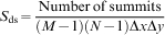
density of summits of the surface S _ds: this is the number of summits of a unit sampling area

ii.

texture aspect ratio of the surface S _tr: this is a parameter used to identify texture strength, that is, uniformity of texture aspect. In principle, the texture aspect ratio has a value between 0 and 1. A value nearer to 1 indicates uniform texture in all directions.

Hybrid parameters (which is a combination of both amplitude and spacing properties):

root mean square slope of the surface S _dq: this is the root mean square value of the surface slope within the sampling area.

Volume family:

core void volume of the surface V _vc: a core void volume is enclosed from 10 to 80% of the surface bearing area and normalised to the unit sampling area.

In this study, therefore, a different type of model for atmospheric corrosion is developed, which involves surface roughness parameters and can be used for corrosion loss determination. This method is eventually expected to be used in situations where the other atmospheric corrosion monitoring methods would not be appropriate.

Experimental

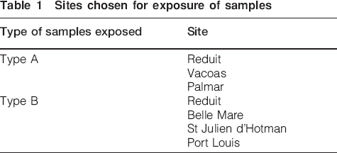
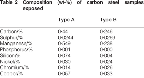
Two types of commercially available carbon steel samples (types A and B) were exposed outdoors at six sites, in Mauritius, according to BS EN ISO 8565.18 The sites chosen are listed in Table 1 and shown in Fig. 1.19 These two types of carbon steel samples vary in their composition. This variation would help the modelling proposed in the paper. The composition (wt-%) of the main alloying elements in the carbon steel used is shown in Table 2.

Figure 1

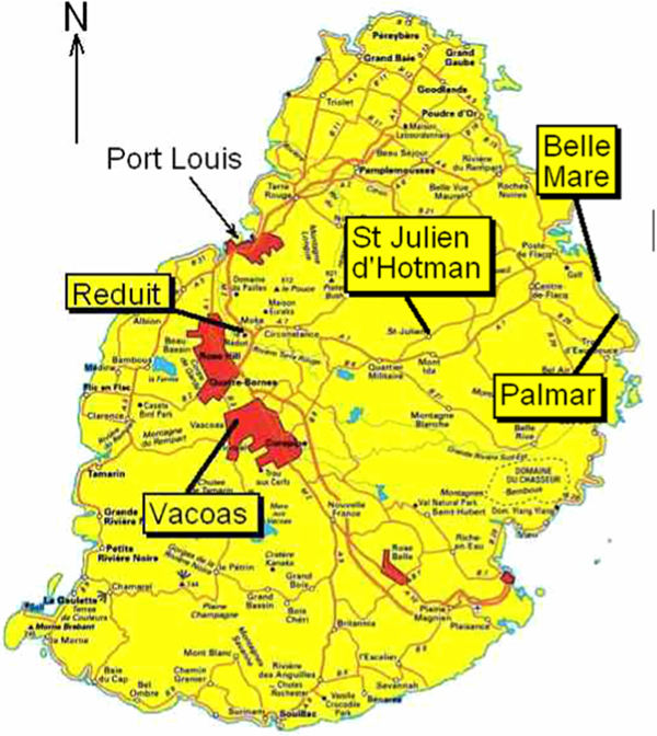
Map of Mauritius showing selected sites 18

Table 1

Sites chosen for exposure of samples

Type of samples exposed	Site
Type A	Reduit
	Vacoas
	Palmar
Type B	Reduit
	Belle Mare
	St Julien d'Hotman
	Port Louis

Table 2

Composition (wt-%) of carbon steel samples exposed

	Type A	Type B
Carbon/%	0·44	0·246
Sulphur/%	0·0244	0·0269
Manganese/%	0·549	0·238
Phosphorus/%	0·001	0·000
Silicon/%	0·074	0·004
Nickel/%	0·030	0·024
Chromium/%	0·014	0·026
Copper/%	0·057	0·033

Both types of samples were cleaned and polished before exposure, and their surfaces showed an average 3D mean roughness of 1·4 μm. Type A samples were removed in sets of three at approximate intervals of 1½, 3, 6, 9, 12, 15 and 18 months for mass loss determination. Type B samples were, on their side, removed in sets of four at approximate time intervals of 2½, 7, 12 and 19 months. Additional samples were retrieved from the exposure racks for each of the removals. These samples were cut to the required size for the analysis of the rust layer through scanning electron microscopy (SEM) images.

When the samples were removed after exposure, they were cleaned for determining the mass loss. This consisted of light mechanical cleaning to remove loose corrosion products followed by chemical cleaning according to BS 7545.20 The samples were cleaned in a sodium hydroxide solution to which zinc was added at 85°C for 30 min.

After cleaning, corroded samples were randomly selected for analysis of the topography of the metal surface. Figure 2 shows the region in which the surface roughness measurements were taken on the samples. To ensure that reliable results are obtained, three sets of readings were taken for each sample in three different parts of the region considered. Each set of reading was taken over an area of 15×15 mm with a cutoff length of 2·5 mm. The TalySurf Series 2 profilometer from Taylor and Hobson was used for this purpose.

Figure 2

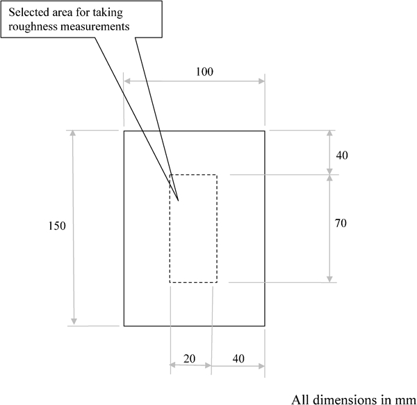
Region in which surface roughness measurements were taken

The roughness parameters were then compared to the respective corrosion loss (μm) of the sample, obtained through mass loss analysis, so as to:

provide explanation on the atmospheric corrosion behaviour of carbon steel

ii.

develop a model for the atmospheric corrosion degradation through surface roughness characteristics of the corroded metal surface.

Results

Mass loss analysis

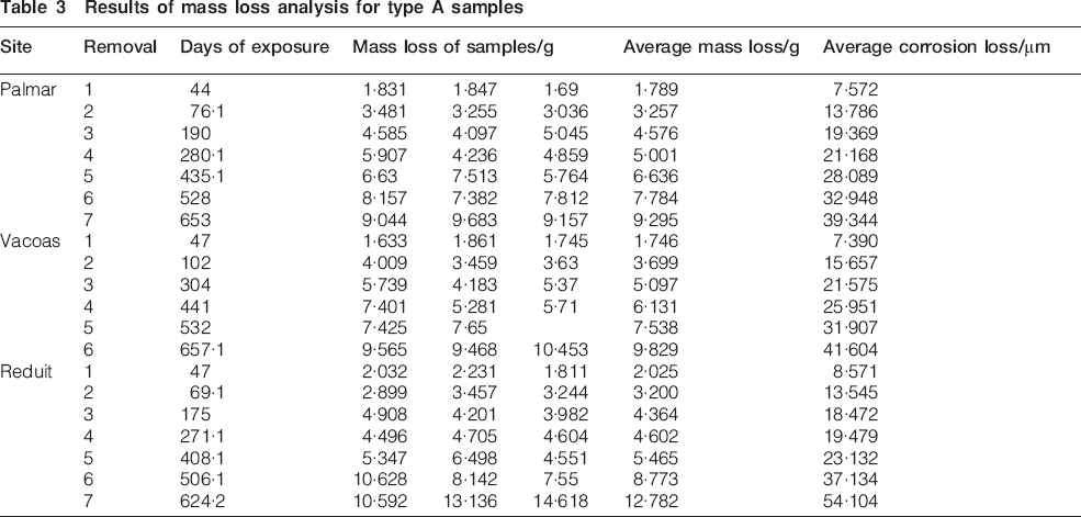
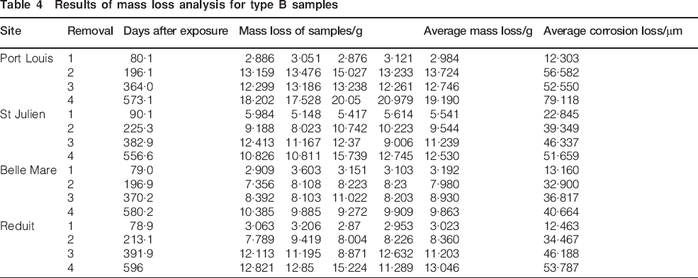
The results of the mass loss analysis are shown in Table 3 Tables 3 and 4. It can be observed that the mass loss increases with time. However, it can also be deduced that the corrosion rate is not constant but rather decreases with time of exposure.

Table 3

Results of mass loss analysis for type A samples

Site	Removal	Days of exposure	Mass loss of samples/g			Average mass loss/g	Average corrosion loss/μm
Palmar	1	44	1·831	1·847	1·69	1·789	7·572
	2	76·1	3·481	3·255	3·036	3·257	13·786
	3	190	4·585	4·097	5·045	4·576	19·369
	4	280·1	5·907	4·236	4·859	5·001	21·168
	5	435·1	6·63	7·513	5·764	6·636	28·089
	6	528	8·157	7·382	7·812	7·784	32·948
	7	653	9·044	9·683	9·157	9·295	39·344
Vacoas	1	47	1·633	1·861	1·745	1·746	7·390
	2	102	4·009	3·459	3·63	3·699	15·657
	3	304	5·739	4·183	5·37	5·097	21·575
	4	441	7·401	5·281	5·71	6·131	25·951
	5	532	7·425	7·65		7·538	31·907
	6	657·1	9·565	9·468	10·453	9·829	41·604
Reduit	1	47	2·032	2·231	1·811	2·025	8·571
	2	69·1	2·899	3·457	3·244	3·200	13·545
	3	175	4·908	4·201	3·982	4·364	18·472
	4	271·1	4·496	4·705	4·604	4·602	19·479
	5	408·1	5·347	6·498	4·551	5·465	23·132
	6	506·1	10·628	8·142	7·55	8·773	37·134
	7	624·2	10·592	13·136	14·618	12·782	54·104

Table 4

Results of mass loss analysis for type B samples

Site	Removal	Days after exposure	Mass loss of samples/g				Average mass loss/g	Average corrosion loss/μm
Port Louis	1	80·1	2·886	3·051	2·876	3·121	2·984	12·303
	2	196·1	13·159	13·476	15·027	13·233	13·724	56·582
	3	364·0	12·299	13·186	13·238	12·261	12·746	52·550
	4	573·1	18·202	17·528	20·05	20·979	19·190	79·118
St Julien	1	90·1	5·984	5·148	5·417	5·614	5·541	22·845
	2	225·3	9·188	8·023	10·742	10·223	9·544	39·349
	3	382·9	12·413	11·167	12·37	9·006	11·239	46·337
	4	556·6	10·826	10·811	15·739	12·745	12·530	51·659
Belle Mare	1	79·0	2·909	3·603	3·151	3·103	3·192	13·160
	2	196·9	7·356	8·108	8·223	8·23	7·980	32·900
	3	370·2	8·392	8·103	11·022	8·203	8·930	36·817
	4	580·2	10·385	9·885	9·272	9·909	9·863	40·664
Reduit	1	78·9	3·063	3·206	2·87	2·953	3·023	12·463
	2	213·1	7·789	9·419	8·004	8·226	8·360	34·467
	3	391·9	12·113	11·195	8·871	12·632	11·203	46·188
	4	596	12·821	12·85	15·224	11·289	13·046	53·787

Results from SEM

The SEM images were taken for the samples at the sites considered. Those for the site at Port Louis observed after the first and third removals are shown in Fig. 3. It can be clearly observed that, initially, the rust layer is much more porous than after 1 year of exposure. However, though the rust layer becomes more protective with time, cracks are also formed, which keeps the corrosion rate at a significant value.

Figure 3

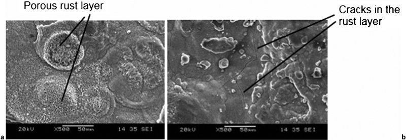
Images (SEM) for site at Port Louis

Roughness parameters

Figure 4 shows the 3D surface texture of a sample from Port Louis taken after 80·1 and 364 days of exposure. Figure 5 Figures 5 and 6 show the respective 2D profiles in the x and y directions.

Figure 4

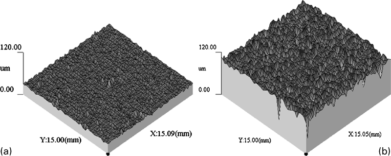
Three-dimensional surface texture of samples exposed at Port Louis after levelling and filtration

Figure 5

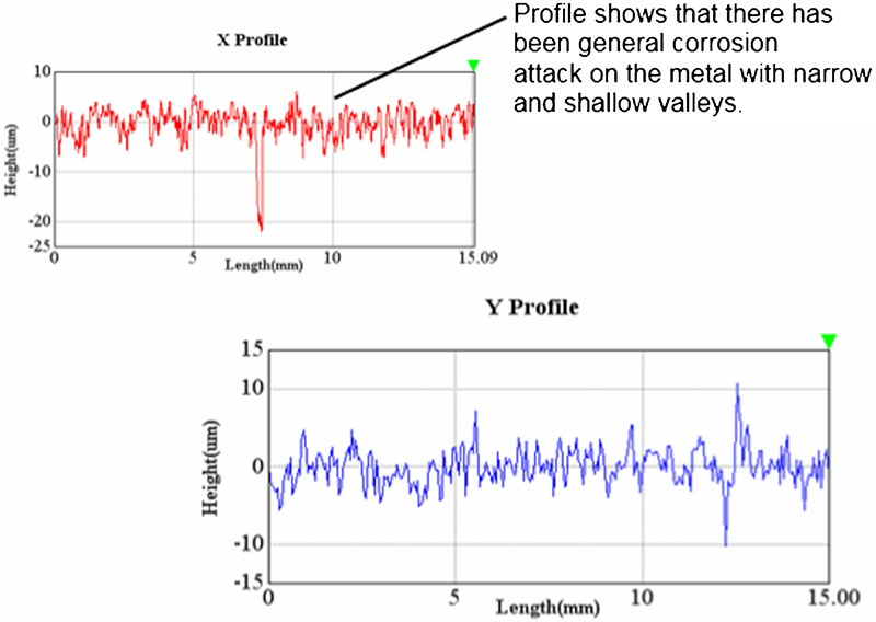
Two-dimensional profile for sample from Port Louis taken after 80·1 days of exposure

Figure 6

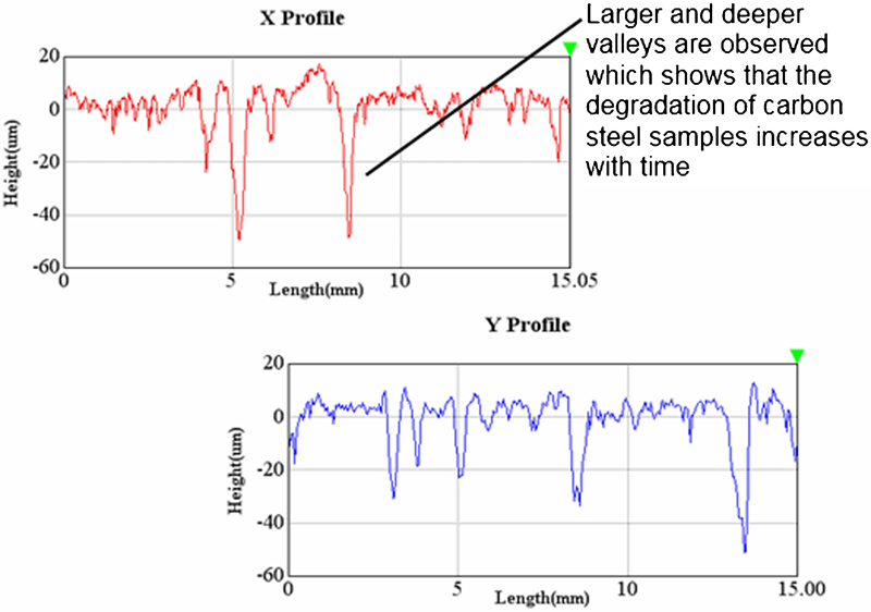
Two-dimensional profile for sample from Port Louis taken after 364 days of exposure

The results for the variation of the roughness parameters (taking into consideration all the sites) with corrosion loss (μm) are shown in Figure 7 Figure 8 Figure 9 Figure 10 Figure 11 Figure 12 Figs. 7-14.

Figure 7

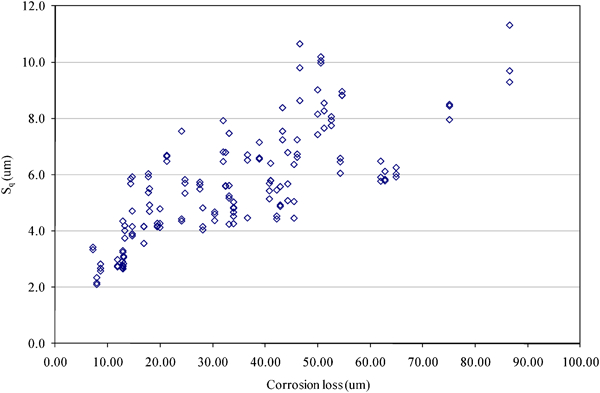
Graph of S _q against corrosion loss

Figure 8

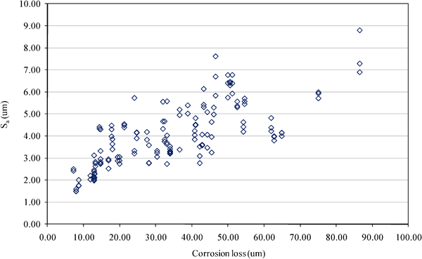
Graph of S _a against corrosion loss

Figure 9

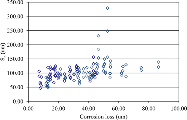
Graph of S _z against corrosion loss

Figure 10

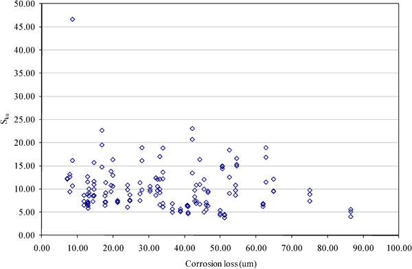
Graph of S _ku against corrosion loss

Figure 11

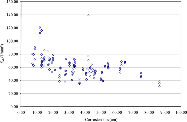
Graph of S _ds against corrosion loss

Figure 12

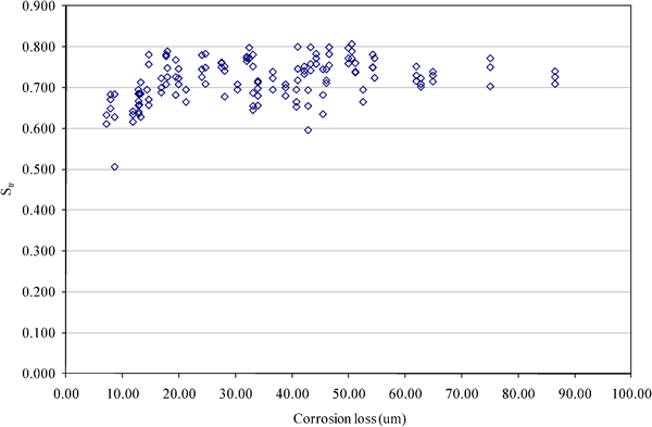
Graph of S _tr against corrosion loss

Figure 14

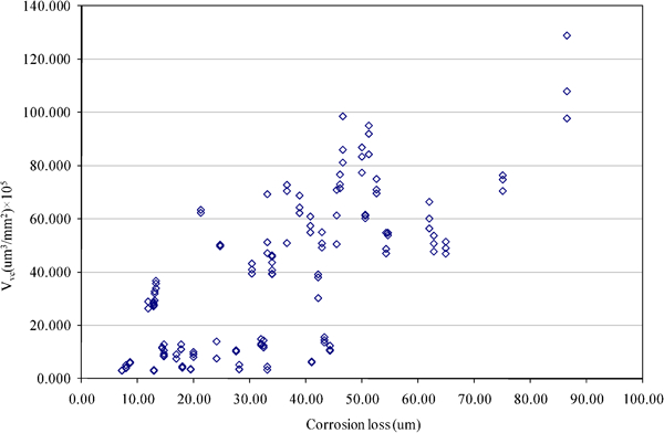
Graph of V _vc against corrosion loss

Amplitude parameters

Mean roughness and root mean square deviation of surface

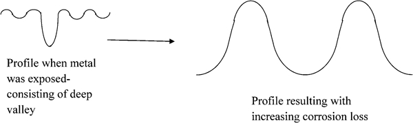
The S _a and S _q parameters represent an overall measure of the texture comprising the surface. S _a can be determined through equation (1)21 (1) where M is the number of points per profile, N is the number of profiles and η(x,y) is the data set for the profile. S _q is defined as the root mean square value of the surface departures within the sampling area. They, therefore, give a good indication of the surface departures within the sampling area, and this can be observed on the metal surface.

Visual inspection of the cleaned samples has shown an increasing surface roughness with time. Figure 5 Figures 5 and 6 confirm these observations with deeper valleys being formed on the metal surface left to corrode for a longer period of time. Figure 7 Figures 7 and 8 also show that the S _a and S _q parameters have a general tendency to increase with the increase in corrosion loss and, as a result, with time of exposure.

It can therefore be deduced that the surfaces of the base metal initially experience general non-uniform corrosion with pits spread over the whole sample area. With the increase in corrosion loss, the corrodants cumulatively degrade the surface, and as a result, the sizes of the summits and valleys increase. This most probably leads to the trend shown in Figure 7 Figs. 7 and 8.

Height deviation between lowest and highest points of surface

It represents an extreme parameter. However, it is expected to have the same behaviour as S _a and S _q, and this is shown in Fig. 9.

Kurtosis of topography height distribution

S _ku indicates the presence of sharp peaks or deep valleys on the surface. A value of >3 indicates the occurrence of sharp peaks or deep valleys, a value of 3 indicates a Gaussian surface and a value of <3 indicates a flat top or well spread surface.

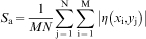
From the graph of S _ku against corrosion loss in Fig. 10, it can be seen that there is one S _ku value, which is very high (46·68). This could have resulted from the presence of inordinately very high peaks or deep valleys on the metal surface. Otherwise, there is a general tendency for the S _ku value to decrease with corrosion loss and approach the value of 3. The initial high values of S _ku could have resulted due to corrosion attack, which can be localised when the metal is exposed to the atmosphere.22 With time, the rust layer becomes more protective, and the corrosion mechanism results due to the diffusion of corrodants in the rust layer. This produces a surface profile, which tends towards a Gaussian surface texture. The variation of the surface profile is illustrated in Fig. 15, taking into consideration the variation in S _a, S _q and S _ku.

Figure 15

Variation in surface profile

Spatial parameters

Density of summits of surface

S _ds can be calculated from equation (2)21 (2) From Fig. 11, it can be observed that the density of summits S _ds has a tendency to decrease with the increase in corrosion loss. This can be explained by the fact that, initially, the atmospheric corrodants would lead to a generalised attack on the surface due to a very thin and unprotective rust layer, and hence, a greater number of summits and valleys are formed but which are small in size. This can be observed in Fig. 4. With time, as the rust layer becomes more protective, the corrosion attack is decreased due to the lesser number of channels available in the rust layer for the corrosion reaction to take place. The formation of cracks in the rust layer tends to increase the number of these channels; however, the resulting effect still leads to an overall decrease in the corrosion rate. Diffusion becomes the mechanism of the corrosion reaction.

Taking into consideration the 2D profiles in Figure 5 Figs. 5 and 6, the formation of cracks in the rust layer (Fig. 3), the variation of the roughness parameters already considered and that diffusion is the corrosion mechanism, the situation can be represented as shown in Fig. 16. With time, the rust layer becomes protective, and the cracks together with the pores present enables the corrodants to corrode the base metal, and this leads to the formation of larger summits and valleys. This would obviously lead to a decrease in the total amount of peaks per unit area, and hence, the S _ds value decreases with time.

Figure 16

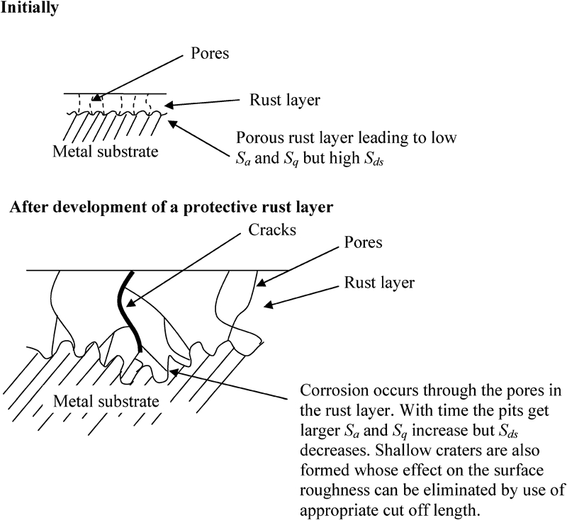
Behaviour of rust layer in atmospheric corrosion exposures

Texture aspect ratio of surface

For a surface with a dominant lay, the S _tr parameter will tend towards 0·00, whereas a spatially isotropic texture will result in an S _tr of 1·00. As shown in Fig. 12, the S _tr values for the corroded surfaces are nearer to 1. Therefore, it can be deduced that in the corrosion attack, the formation of pores and cracks (at a later stage) is random in nature.

Hybrid parameters

Root mean square slope of surface

From Fig. 13, it can be seen that S _dq increases with corrosion loss. This implies that the surface of the peaks becomes steeper as the metal gets corroded. This is in line with the previous results with a shallow profile when the metal is exposed, as shown in Fig. 16, and then the formation of larger profiles on the base metal as the corrosion process continues. These profiles would obviously be steeper than the shallow ones developed initially.

Figure 13

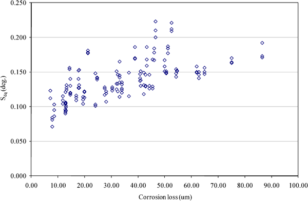
Graph of S _dq against corrosion loss

Functional volume family

The functional volume family of parameters are used extensively and specifically for tribology applications. However, this family of parameters can be of help in this study; the volume in the valleys can give an indication of the amount of electrolyte deep down the pores that get in contact with the metal and produce the corrosion reaction.

One such parameter is the core void volume V _vc, and it is enclosed from 10 to 80% of the surface bearing area and normalised to the unit sampling area. Since the corrosion reaction takes place deep down in the pores of the rust layer, therefore, it is expected that the corrosion rate would relate well with V _vc. Figure 17 shows a very simplified model of the corrosion of carbon steel in a wet state. Corrosion occurs deep down the pores/cracks, and the metal in that region gets consumed. The amount corrosion would depend on the amount of metal and electrolyte interaction. Hence, it can be expected that V _vc relates well with corrosion loss.

Figure 17

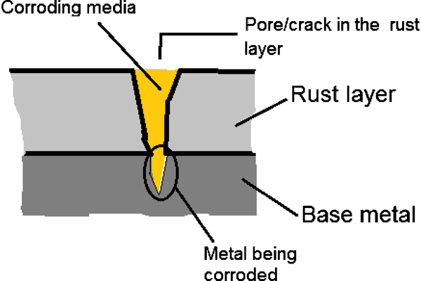
Simple model of corroding carbon steel

From Fig. 14, it can be observed that the core void volume gets larger with corrosion loss, which suggests that the valleys formed get larger in size as the metal corrodes. V _vc, however, does not show any specific trend with corrosion loss.

Analysis of results

The results for both types A and B are used together to develop the model for the corrosion loss of carbon steel in the Mauritian atmosphere. The model to be developed was inspired from:

the exponential law equation commonly used in gravimetric studies of carbon steel 17 17,23 (3) where C is the corrosion loss (μm), and t is the time (months). A is generally considered as a measure of the initial reactivity of the material with the environment, and it is numerically equivalent to the corrosion loss when time is unity. The exponent B is a measure of the protective ability of the corrosion products formed.24

ii.

dose–response functions that are also being commonly used nowadays to predict the expected corrosion damage rate.24 In the dose–response function, the rate of corrosion is termed ‘response’ R, and the atmospheric corrodant is termed the ‘dose’ C. Mathematically (4) where the square brackets indicate concentration, i is the index for the corrodant and f is the function relating the extent of the damage to the specified dose.

Taking into consideration these models for atmospheric corrosion modelling, the following was chosen for development using multiple regression analysis (5) where C is the corrosion loss (μm), k is a constant and t is the time of exposure (days).

Roughness parameters

The roughness parameters would be used as independent variables. Some of the parameters such as V _vc are expected to show some extent of correlation with corrosion loss since, as indicated above, they are directly related to the atmospheric corrosion process. Others, like S _dq and S _tr, just show some surface profile changes, which would not necessarily be related to the corrosion process.

Statistical analysis

There was no grouping of data, and as a result, there were 150 sets of readings. The following independent variables were preselected for the model: ln (days of exposure), carbon content of the carbon steel samples, S _a, S _q, S _ku, S _z, S _ds, S _tr, S _dq and V _vc.

The carbon content of the carbon steel samples is also considered as an independent variable because it has been reported25 that the carbon content can be regarded as a factor affecting corrosion.

The dependent variable was taken to be ln (corrosion loss).

To keep the model simple and at the same time representative of the results obtained, only three independent variables and a linear model were considered. The data distribution was first checked, and then the model was developed sequentially.

Checking of distribution

Missing value

There was no missing value.

Ratio of cases to independent variables

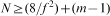
For the present analysis, the model would consist of a maximum of three independent variables for simplicity. Equation (6) was used as the rule of thumb to find whether there are enough cases for the amount of IVs to be included in the model26 (6) where N is the required sample size, m is the number of IVs and f2 = 0·02, 0·15 and 0·35 for small, medium and large effects respectively.

With three IVs, f2 was assumed to be 0·15, and the required sample size was found to be at least 57 to observe medium effects, which is the case with the present study.

Normality

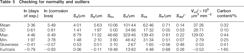
The distribution of the means of the groups of variables was therefore checked for normality. Table 5 shows the results obtained. It can be observed from Table 5 that the data for S _z, S _ds and S _tr have a high value for skewness and kurtosis, and therefore, they are good candidates for transformation. The data for carbon content have a high value for kurtosis. However, it consists of only two values (0·246 and 0·44) and, therefore, would not be considered for transformation. The other independent variables and the dependent variable can be considered to be normal.

Table 5

Checking for normality and outliers

	ln (days of exp.)	ln (corrosion loss)	S _a/μm	S _q/μm	S _ku	S _z/μm	S _ds	S _tr/μm	S _dq/°	V _vc/×10⁵ μm3 mm⁻²	Carbon content/%
Mean	3·36	5·49	4·01	5·63	10·06	101·44	62·46	0·71	0·14	37·26	0·32
SD	0·61	0·81	1·41	1·97	5·00	34·96	17·32	0·05	0·03	28·71	0·10
Max.	4·46	6·49	8·79	11·32	46·68	329·46	139·43	0·81	0·22	129·00	0·44
Min.	1·97	3·78	1·48	2·10	3·80	46·42	31·34	0·51	0·07	2·79	0·25
Skewness	−0·41	−0·57	0·53	0·51	3·10	2·67	1·65	−0·56	0·48	0·53	0·41
Kurtosis	−0·79	−0·93	0·06	−0·11	18·48	13·92	4·48	0·68	0·28	−0·53	−1·85

S _z, S _ds and S _ku were transformed to ln S _z, ln S _ds and ln S_ku, and Table 6 shows the check for normality for the transformed variables.

Table 6

Checking for normality and outliers for transformed variables

	ln S _ku	ln S _z/μm	ln S _ds
Mean	2·22	4·57	4·10
SD	0·41	0·30	0·25
Max.	3·84	5·80	4·94
Min.	1·33	3·84	3·44
Skewness	0·49	0·28	0·43
Kurtosis	0·70	1·99	1·27

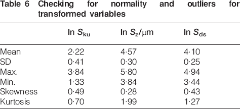
It can be observed that there is a large amelioration in the normality of the distribution of the variables.

Outliers among independent variables and dependent variable

For each type of variable, the distribution was checked for outliers. The presence of outliers is detected with standardised scores in excess of 3·29 (p<0·001, two-tailed test) standard deviations below or above the mean. From Table 5 Tables 5 and 6, outliers were found for S _a, ln S _ku, ln S _z, ln S _ds, S _tr and carbon content. However, the outliers would not be deleted because they represent values that can occur in certain specific situations.

After checking for normality and outliers, the presence of homoscedasticity and linearity was checked using residual plots. No clear cases of the presence of heteroscedasticity or non-linearity were observed.

Development of model

SPSS 13·0 was used to perform the statistical analysis. The following abbreviations were therefore used for the dependent variable and the independent variables:

•.

ln t: ln (days of exposure)

•.

CC: carbon content

•.

Sa: S _a

•.

Sq: S _q

•.

ln Sku: ln S _ku

•.

ln Sz: ln S _z

•.

ln Sds: ln S _ds

•.

Str: S _tr

•.

Sdq: S _dq

•.

Vvc: V _vc

•.

ln C: ln (corrosion loss).

Estimating regression model and assessing overall model fit

A sequential procedure was employed to select variables for inclusion in the regression equation.

Models 1-10, as shown in Table 7, were initially tested with the aim of obtaining the most appropriate simple and easy to use equation. ln t was considered as the common parameter to be included in all the regression equations because it was considered as the parameter on which the corrosion loss would mainly depend.

Table 7

Models 1-10

Model no.	Description	R value
1	ln C = b ₀+b ₁ln t	0·823
2	ln C = b ₀+b ₁ln t+b ₂Sa	0·871
3	ln C = b ₀+b ₁ln t+b ₂Sq	0·876
4	ln C = b ₀+b ₁ln t+b ₂ln Sku	0·826
5	ln C = b ₀+b ₁ln t+b ₂ln Sz	0·834
6	ln C = b ₀+b ₁ln t+b ₂ln Sds	0·830
7	ln C = b ₀+b ₁ln t+b ₂ln Str	0·824
8	ln C = b ₀+b ₁ln t+b ₂Sdq	0·868
9	ln C = b ₀+b ₁ln t+b ₂Vvc	0·927
10	ln C = b ₀+b ₁ln t+b ₂CC	0·923

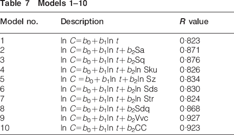
It can be noticed that model 9 has the highest R value. In order to validate this model for further improvement, the following properties were checked:

multicollinearity

ii.

multivariate outliers (through Mahalanobis distance)

iii.

normal probability and partial plots.

It was observed that multicollinearity was not evident, and there was no outlier. The normal probability plot is shown in Fig. 18. The normal probability and partial plots showed that there is no evidence of heteroscedasticity or non-linearity in the model. Moreover, improvement in the normal probability plot is expected with the addition of a new independent variable in the model.

Figure 18

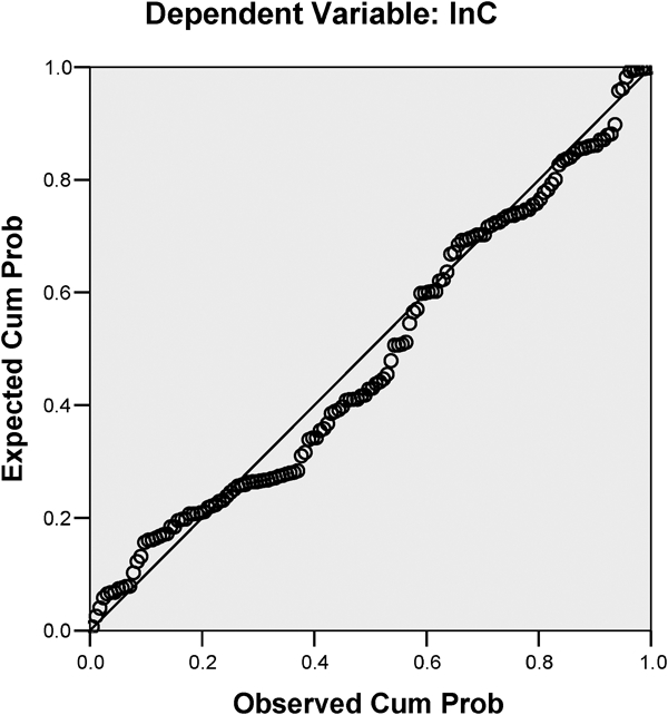
Normal probability plot for model 9

Therefore, model 9 was selected for further analysis.

Using three independent variables

One additional and final independent variable is now inserted to the regression equation to improve it and at the same time keep it simple for use. The investigated models 11-18 are shown in Table 8.

Table 8

Models 11-18

Model no.	Description	R value
11	ln C = b ₀+b ₁ln t+b ₂Vvc+b ₃Sa	0·927
12	ln C = b ₀+b ₁ln t+b ₂Vvc+b ₃Sq	0·928
13	ln C = b ₀+b ₁ln t+b ₂Vvc+b ₃ln Sku	0·933
14	ln C = b ₀+b ₁ln t+b ₂Vvc+b ₃ln Sz	0·927
15	ln C = b ₀+b ₁ln t+b ₂Vvc+b ₃ln Sds	0·928
16	ln C = b ₀+b ₁ln t+b ₂Vvc+b ₃Str	0·930
17	ln C = b ₀+b ₁ln t+b ₂Vvc+b ₃Sdq	0·927
18	ln C = b ₀+b ₁ln t+b ₂Vvc+b ₂CC	0·933

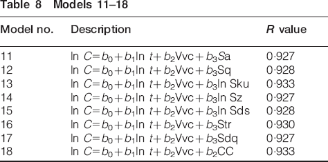
Models 13 and 18 were selected as they have the highest R value. To select one of these two, further statistical tests were performed on:

linearity, homoscedasticity, normality and outliers

ii.

significance of the regression

iii.

significance of regression coefficients

iv.

improvement in fit obtained from additional explanatory variable

multicollinearity.

It was concluded that model 18 is better than model 13 because the latter consists of a regression coefficient that is not significant. Moreover, the third independent variable improved the other statistical parameters used to evaluate the model. The model, as shown in equation (7), showed the presence of normality and linearity and the absence of homoscedasticity, outliers and homoscedasticity. The regression and the regression coefficients are both significant. There is also a significant improvement in fit from the additional variable added. The normal probability plot for model 18 is shown in Fig. 19, which is an improvement on model 9.

Figure 19

Normal probability plot for model 13

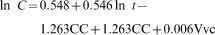
The selected model is, therefore, as shown below (7) where ln C refers to ln (corrosion loss), ln t refers to ln (days of exposure), CC refers to carbon content and Vvc refers to V _vc.

It can be observed that V _vc has a positive effect on corrosion rate, which is quite normal, as it will represent the amount of corrodants in the rust layer. Carbon content has a negative impact on the corrosion rate, as expected. The average corrosion losses in the two types of samples considered are plotted separately against time of exposure in Fig. 20. It can indeed be observed that carbon content does have an effect on the atmospheric corrosion behaviour of the metals considered.

Figure 20

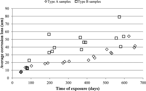
Graph of average corrosion loss against time of exposure for two types of samples considered

Conclusions

From the results of the 3D surface roughness analysis of the base metal of the corroded samples, the following can be concluded.

The uneven general corrosion on the carbon steel surface produces peak and valley structures on the base metal, which is spatially isotropic. This can be the result of the randomness of the corrosion attack, the formation of pores and the formation of cracks.

This paper analyses the skyward surfaces of the corroded specimens. During the time span of corrosion studies, the average roughness of the surface increased with the increase in corrosion loss.

At the start of the corrosion process, the corrosion attack is more severe at some localised places, which results in the presence of some inordinately high peaks or valleys on the surface. As already stated earlier, this type of behaviour has been reported by Tabachnick and Fidell.26 With time, the surface becomes coated with the rust layer that is porous. The corrosion process proceeds through pores and cracks, and the surface texture becomes more of a Gaussian type.

The increase in the size of the peak and valley structures with increasing corrosion loss is confirmed by a general increase in the core void volume. Larger peaks and valleys also lead to a decrease in the number of peaks or summits.

The model obtained for the corrosion loss is as obtained in equation (7). It should be noted that there are various other factors linked with metallurgy, such as the amount of sulphur in the metal surface, which have not been taken into consideration but could have an influence on corrosion rate.

The high R value obtained for the simple linear model suggests that surface roughness analysis can be used as an alternative method to the traditional weight loss method for determining the amount of corrosion degradation in certain specific situations. This model, for example, would be very useful in small countries, like Mauritius, which consists of microclimates and in which much research has not been performed. With the results of the present study, surface roughness of already corroded carbon steel items can be determined in situ, and the corrosion degradation at the site can be found. Otherwise, installed metal structures that cannot be brought to the laboratory can be monitored for maintenance purposes.

A better correlation can be obtained using other types of equations or other techniques, such as neural networks.27 Equation (6) also suggests that time of exposure and carbon content of the carbon steel samples are major factors affecting atmospheric corrosion loss. V _vc, on the other hand, is a most significant roughness parameter.

References

McKenzie

Vassie

: ‘Use of weight loss coupons and electrical resistance probes in atmospheric corrosion tests’, Br. Corros. J. 1985 20 117–124.

Castano

Botero

Restrepo

Agudelo

Correa

Echeverria

: ‘Atmospheric corrosion of carbon steel in Columbia’, Corros. Sci. 2010 52 216–223.

Natesan

Venkatachari

Palaniswamy

: ‘Kinetics of atmospheric corrosion of mild steel, zinc galvanised iron and aluminium at 10 exposure stations in India’, Corros. Sci. 2006 48, 3584-3608.

Lan

TTN

Thoa

NTP

Nishimura

Tujino

Yokoi

Maeda

: ‘Atmospheric corrosion of carbon steel under field exposure in the southern part of Vietnam’, Corros. Sci. 2006 48 179–192.

Natesan

Venkatachari

Palaniswamy

: ‘Corrosivity and durability maps of India’, Corros. Prev. Control 2005 52 43–55.

Hassiotis

Petropoulos

: ‘Influence of surface roughness on corrosion resistance of turned carbon steel parts’, Int. J. Mach. Mach. Mater. 2006 1 202–212.

Lin

M.-C

Lin

S.-C

Lee

T.-H

Huang

H.-H

: ‘Surface analysis and corrosion resistance of different stainless steel orthodontic brackets in artificial saliva’, Angle Orthod. 2006 76 322–329.

Zhang

Yang

: ‘Microstructures and properties of aluminum film and its effect on corrosion resistance of AZ31B substrate’, Trans. Nonferrous Met. Soc. China 2008 18 s312–s317.

Belous

Éiduk

YuYa

Ponomareva

ÉP

: ‘The effect of surface roughness on corrosion resistance of ceramics’, Glass Ceram. 1985 42 417–420.

10.

Moayed

Laycock

Newman

: ‘Dependence of the critical pitting temperature on surface roughness’, Corros. Sci. 2003 45, 1203-1216.

11.

Nairn

Skennerton

Atrens

: ‘Comparative atmospheric corrosion of primary and cold rolled copper in Australia’, J. Mater. Sci. 2003 38 995–1005.

12.

Petropopulos

Pandazaras

: Ind. Lubr. Tribol. 2003 55 128–136.

13.

Hoerle

Mazaudier

Dillman

Santarini

: ‘Advances in understanding atmospheric corrosion of iron. II. Mechanistic modelling of wet–dry cycles’, Corros. Sci. 2004 46, 1431-1465.

14.

Eyring

Robertson

Chu

Andersen

: ‘Atmospheric corrosion (theoretical model)’, Proc. Natl. Acad. Sci. USA 1974 71 245–247.

15.

Ohtsuka

Komatsu

: ‘Enhancement of electric conductivity of the rust layer by adsorption of water’, Corros. Sci. 2005 47, 2571-2577.

16.

Burakowski

Weirzchon

: ‘Surface engineering of metal: principle, equipment, technologies’168; 1998

Boca Raton, FL

CRC Press.

17.

Wei

: ‘Atmospheric corrosion of carbon steels and weathering steels in Taiwan’, Br. Corros. J. 1991 26 209–214.

18.

‘Metals and alloys: atmospheric corrosion testing. General requirement for field tests’

BS EN ISO 8565

BSI

London, UK

1995.

19.

Venkatasamy

: ‘Atlas for Mauritius’ 1st edn; 1991

Rose Hill

The Editions de l'Ocean Indien.

20.

‘Method of removal of corrosion products from corrosion tests specimens of metals and alloys’

BS 7545, BSI, London, UK 1991.

21.

Blunt

Jiang

: ‘Advanced techniques for assessment of surface topography – development of the basis for 3D surface texture standards “Surfstand” (Kogan Page Science paper edition)’17–43; 2003

London

Butterworth-Heinemann.

22.

Han

Wang

: ‘Characterisation of initial atmospheric corrosion carbon steels by field exposure and laboratory simulation’, Corros. Sci. 2007 49, 2920-2935.

23.

Morcillo

Feliu

Simancas

: ‘Deviation from bilogarithmic law for atmospheric corrosion of steel’, Br. Corros. J. 1993 28 50–52.

24.

Graedel

Leygraf

: ‘Atmospheric corrosion’101–102; 2000

New York

Wiley Interscience.

25.

Roy

: ‘Corrosion of steel in tropical marine atmosphere’, Br. Corros. J. 1994 29 287–291.

26.

Tabachnick

Fidell

: ‘Using multivariate statistics’ 5th edn1–194; 2007

Boston, MA

Pearson International Edition.

27.

Kenny

Paredes

RSC

de Lacerda

Sica

de Souza

Lazaris

: ‘Artificial neural network corrosion modelling for metals in an equatorial climate’, Corros. Sci. 2009 51, 2266-2278.