Explicit spreadsheet method for predicting internal corrosion in two galvanically coupled long pipes

Abstract

Some piping systems used in deep water oil production, including risers and flow lines, or those used for sea water piping, are galvanically coupled. The potential and current distributions in the pipe's axial direction have traditionally been predicted using either an analytical expression assuming linear polarisation kinetics or a numerical modelling using polarisation data or corresponding Tafel equations as the model input. The analytical expressions are invalid when the polarisation behaviour is non-linear, as often is the case. The numerical method may find limited users because many experimentalists, technicians and practicing engineers often are not used to or experienced with it. This paper reports an explicit four-step procedure that requires only the use of a spreadsheet to obtain the potential and current distributions from the polarisation data, and the results are robust. The predicted potential distribution is compared with those obtained from traditional numerical and analytical methods. In addition, a method developed to scale the pipe diameter is reported.

Keywords

Steel Titanium Alloys Modelling studies Acid corrosion Galvanic corrosion Piping

Introduction

Some piping systems used in oil production offshore, including risers and flow lines, are galvanically coupled. For instance, a portion of carbon steel (CS) piping may be internally cladded with an Inconel alloy (e.g. A625) for protection against internal corrosion, erosion or corrosion fatigue at the touchdown zones.1 ^– 3 The use of such cladding materials can, however, elevate the steel pipe corrosion near the joint with A625, where the galvanic coupling effect is strongest. The galvanic coupling effect is induced by the difference in corrosion potential between the two dissimilar metals. This potential difference drives a current that flows out from the less noble metal surface (e.g. steel) towards the more noble metal surface (e.g. A625). The less noble metal thus acts as the anode and corrodes preferentially, and the more noble metal acts as the cathode where cathodic reactions, such as acid and/or water reduction, take place. The magnitude of the steel corrosion can depend on the type of metals, their polarisation behaviours, relative effective surface areas, geometries and resistivity of the electrolyte.

When galvanic coupling occurs between a steel riser and a titanium stress joint,4 in addition to the preferential corrosion of the steel riser, the hydrogen charging into titanium to form hydride is of great concern. The titanium hydride can enhance the susceptibility of the titanium stress joint to hydrogen embrittlement and corrosion fatigue under cyclic loading conditions.4 ^– 6 Although the hydrogen charging can take place at the exterior surface of the titanium stress joint where cathodic reactions (e.g. water reduction), dominated by the externally applied cathodic protection, take place through sea water,6,7 the methods reported in this paper apply only to the galvanic coupling between the internal surfaces of the piping.4,8 Inside the pipe, the electrolyte can be sweet or sour brines at a normal or elevated temperature.

Sea water piping systems and marine tubular heat exchangers between tubes and tube plates also involve galvanic corrosion between dissimilar metals such as CS, copper–nickel alloys, stainless steels and titanium alloys.9 ^– 11 In sea water piping systems, an older cement lined CS piping may be partly replaced by titanium or a stainless steel. Failures in the cement lining make the CS vulnerable to galvanic corrosion near the coupling.

Dissimilar metals have also been found in piping systems during ship retrofitting. An extensive study was reported where the galvanic potential distribution in two joined pipes of dissimilar metals was measured and discussed for different metallic couplings (titanium or anodised titanium versus 70∶30 copper/nickel with and without calcareous deposits) at different times.12

Both analytical and numerical modellings of potential and current distributions in piping systems of dissimilar metals have been performed in the past. When linear polarisation kinetics can be assumed at the metal surface, two-dimensional13 and one-dimensional (1D) expressions11,14 in closed form are available for predicting the potential and current distributions. It was reported that the 1D expression in the pipe's axial direction can be simplified from the two-dimensionality when D/W<4, where D is the pipe inner diameter and W is the Wagner polarisation parameter with W = R _p/ρ (where R _p is the linear polarisation resistance of the pipe metal in the electrolyte, and ρ is the electrolyte resistivity).11,15

For the system of interest here, such an analytical expression in 1D will only be discussed later in this paper. Although analytical expressions can be very useful and easy to use when the magnitude of polarisation of the two galvanised metals is small (or polarisation kinetics is linear), it becomes invalid when the polarisation behaviours of the two metals are non-linear, as often is the case. For the non-linear polarisation behaviours, numerical methods such as finite element or finite difference are traditionally used to attain the distributions of potential and current in the pipe axial direction,1,11 and either Tafel equations or the actual polarisation data must be used as the model input parameters.

Even though numerical modelling in 1D appears to be straightforward, a software code, either house made or commercially purchased, still has to be used to perform the model simulations. This poses limits to many experimentalists, technicians and practicing engineers who are not used to or experienced with such numerical simulations.

This paper introduces a simple explicit method that every engineering professional can use to obtain the axial potential and current distributions with the need of only a spreadsheet. This paper also presents a scaling method that allows for the charts of potential and current distributions, generated from one given pipe diameter, to be extended for other sizes of pipe diameter. A four-step procedure with an example has been developed to implement the spreadsheet method, and the results obtained from this spreadsheet method are compared with results from traditional analytical and numerical methods and shown to be robust. Merits and limitations of the spreadsheet method are discussed.

Mathematical model

The galvanically coupled piping system to be concerned in this work is schematically shown in Fig. 1, where two dissimilar metallic pipes of uniform inner diameter are joined together at x = 0. The less noble metallic (steel) pipe is placed on the left to the joint (x<0) and the more noble metallic (e.g. nickel alloy, titanium or stainless steel) pipe on the right to the joint (x>0). Only the axial distributions of potential and current are of concern because D/W<4 (to be discussed later).

Figure 1

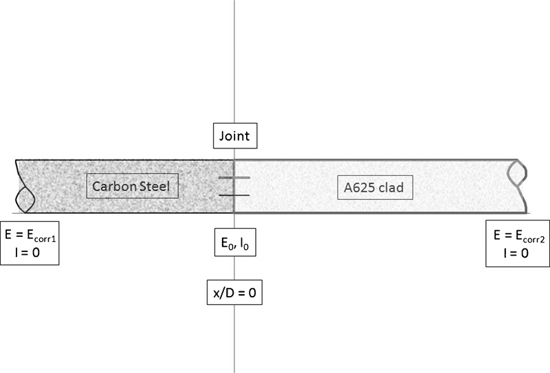
Schematic of model geometry

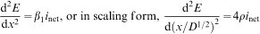
For the galvanic piping system shown in Fig. 1, following Ohm's law, the ionic current that flows in electrolyte across the cross-section of the pipe is (1) where β ₀ = πD ²/4ρ, E is the metal corrosion potential, ρ is the solution resistivity and D is the pipe inner diameter.

When the diameters of the two pipes are the same, charge conservation dictates that (1a) where i _net is the net current density that flows across the metal/solution interface, which is the sum of the anodic (positive) and cathodic (negative) current densities. The anodic and cathodic current densities can be described by the measured polarisation data of the two metals or by the metals’ Tafel equations.

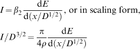
Substituting equation (1) into equation (1a) yields (2) where β ₁ = 4ρ/D is a model parameter relating to solution resistivity and pipe diameter. Since i _net in equation (2) is a function of E only, the chart of E versus x/D ^1/2 does not vary with variation in D. Such a chart is in this work called scaling plot. Similar scaling method in modelling has also been reported elsewhere.16,17

Although the scaling plot for i _net is straightforward, which is i _net versus x/D ^1/2 because i _net is a direct function of E only, the scaling plot for the total current I needs to be derived from equation (1) by (2a) where β ₂ = πD ^1·5/4ρ. The scaling chart for total current I should be plotted as 1/D ^3/2 versus x/D ^1/2. The scaling plots for potential and current will be demonstrated in the next section.

To solve the second order differential equation, equation (2), boundary conditions must be provided. For the interest of this paper, we assume that the two joined pipes are each long enough so that the galvanic effect dies out at a far distance from the joint. At this far distance from the joint, the corrosion potential of each metal reaches its open circuit potential (OCP) E _corr, or E = E _corr, and the axial current flowing in the electrolyte is zero, or dE/dx = 0. dE/dx = 0 is used as the boundary condition at the far end of the simulated pipe geometry (Fig. 1).

Not for the sake of boundary conditions, it is however useful to know that at the far distance from the joint, the net current density at the pipe/electrolyte interface is zero for each pipe, or i _net = 0, and at the pipe joint, both the potential E and the current I must be continuous.

In order to solve equation (2) with an easy to use spreadsheet (as opposed to traditional methods), equation (2) is rearranged as (3) where . To arrive at equation (3), let p = dE/dx (an intermediate variable) so that (d² E/dx ²) = [d(p)/dE](dE/dx) = p[d(p)/dE] = [d(p ²)/2dE]. Since p = I/β ₀ following equation (1), 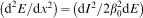and equation (2) can be rearranged to obtained equation (3).

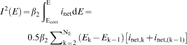
When the polarisation curve of each metal is available, E and i _net are known, so that equation (3) can be integrated to obtain current I by (4) where the integral limit E and the summation limit N _E indicate that I ²(E) is cumulative, starting from a value of zero at the OCP of the metal E _corr. The integration limit E or N _E is not a constant as to be more clearly demonstrated by the spreadsheet later. k = 2, 3, …, N _E, …, N represent the measured data points for either one of the two metals. The summation on the right hand side of equation (4) represents a simple integration (via the trapezoidal rule) from E _corr to E _k. After the integration, the currents I(E) are computed versus E.

Four-step spreadsheet method, with an example

An explicit four-step procedure was developed to guide the use of the spreadsheet method and create the desired graphs, including the axial distributions, against x, of the corrosion potential E, current across the pipe cross-section I and the net current density flowing across the metal/solution interface i _net.

As an example, Fig. 2 shows the polarisation data for steel and A625 in a sweet brine reported elsewhere.18 These data represent a controlled E _j versus a measured i _netj, j = 1, 2, where j = 1 stands for metal 1 (steel), and j = 2 for metal 2 (A625). The solution resistivity is 0·2 Ω m and the pipe inner diameter is 0·2 m.

Figure 2

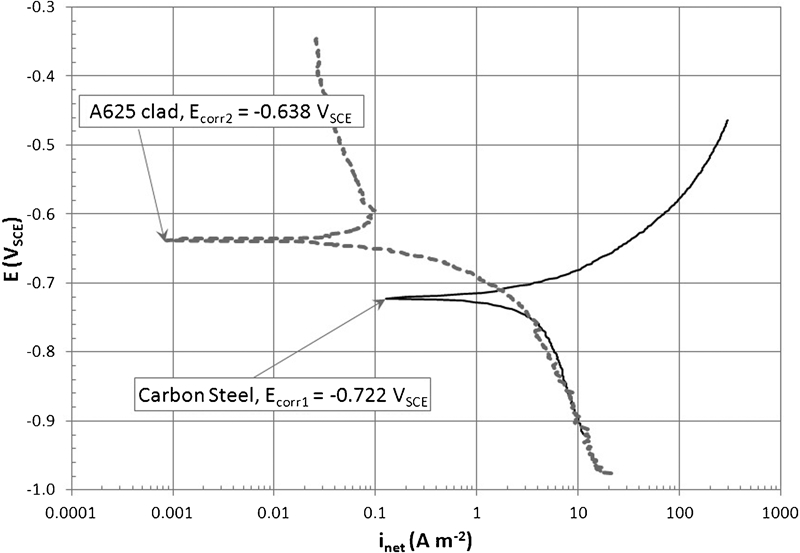
Polarisation curves of CS and A625 in sweet brine1 (potential E versus current density i _net)

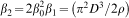
The polarisation data are also presented in Fig. 3, an image of the spreadsheet used in this paper to demonstrate how distributions of the galvanic potential and current are determined and how the spreadsheet method works step by step. In the top first two rows of the spreadsheet, the model global variables are shown including pipe inner diameter D, electrolyte resistivity ρ and β ₀ in equation (1) and β ₂ in equation (4). Below the second row, the field of the spreadsheet is equally divided by the central vertical line; the left portion is for CS, and the right portion is for A625. In each subfield, five columns are sequentially labelled in the third row; for the same column number, the properties (shown by the fourth row) are same for CS and A625. The equations used to determine the parameters in the third and fifth columns are labelled. The spreadsheet method consists of four steps. In the first three steps, the galvanic potential and current are determined. The fourth step is plot of the model results. These four steps are next described in detail.

Figure 3

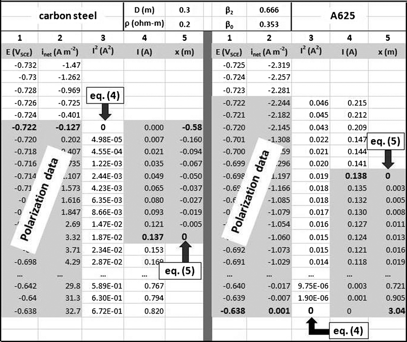
Image of spreadsheet used to determine galvanic potential and current distributions along pipe axial direction

The first step is to determine or locate the OCP for each metal E _corrj. E _corrj can be values measured from the experimental tests before the polarisation scan. Alternatively, it may be located by searching the potential at the smallest absolute value of the measured net current density i _netj for each metal. If the two methods get close values of E _corrj as is usually the case, the values from the latter method are used. When the two methods give appreciably different values, a method is given in a later section to treat such potentials.

Such an OCP for each metal would be located at a far distance from the pipe joint, unaffected by the galvanic coupling. At such a potential, the corresponding net current density for the metal is supposed to be zero. In the experimental measurement, the E value cannot be controlled to make i _netj exactly 0, although the value is very small. For that reason, it is useful to check if the i _netj value from which the E _corrj was determined is a true minimum, located in ‘the bottom of a valley’ of a plot of |i _netj| versus E _j. Figure 2 shows the |i _netj| versus E _j (j = 1, 2) plots, and the minimum |i _netj| is verified to be located in the bottom of each |i _netj| valley. These OCPs and corresponding current densities for CS and A625 are shown in bold in Fig. 3; the more negative OCP is associated with CS, and the more positive OCP with A625. The pipe galvanic potentials can only fall within the range of these two OCPs.

The second step is to integrate each i _netj over E _j between the two OCPs of the two metals, E _corr1 and E _corr2, to obtain a function from equation (4). This results in the third column in Fig. 3 for both CS and A625. At E _corrj, zero current I _j(E) is given by definition. Because the OCPs of CS and A625 are the limits of the galvanic potential range, when integrating with equation (4), the integration shown in Fig. 3 moves downward for CS and upward for A625. The fourth row can be obtained simply by taking the square root of the values in the third column for both CS and A625.

In equation (4), k = 2, …, N _E, …, N _j for metal j (j = 1, 2) represent a subset of all the measured data points for the given metal j. The subset of measured points (E _j, i _netj) is chosen such that E _corr1⩽E _k⩽E _corr2, or the E _k of the chosen points falls between the OCPs of the two metals. It is straightforward to view the integration results in Fig. 3, the spreadsheet. Even though the (E _j, I _j) data may be noisy in fine scales, the integration provides smoother (E _j, I _j) lines, as shown in Fig. 4.

Figure 4

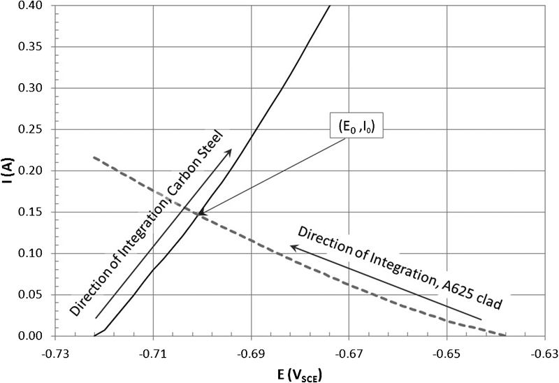
Results of first integration from equation (4): cross-section current I versus potential E curves

The two (E _j, I _j) curves plotted on one diagram, one curve for CS and one for A625, should intersect, each curve going from E _corr1 to E _corr2. The intersection of those two lines occurs at the point (E ₀, I ₀) that represents the potential and the current at the pipe joint with x = 0 shown in Fig. 1. Figure 4 shows an example of this plot, with the indicated crossover point (E ₀, I ₀). It is important to locate this crossover point before proceeding to the next step. The values at the crossover point are shown in bold in the fourth column in Fig. 3 for both CS and A625.

The third step is to integrate 1/I _j over E _j from E ₀ to E _corrj, to get x _j for each metal j. The basis of this integration is equation (1), and (5) Again, x _j(E) is a cumulative function, and the N _j represent the same subset of measured points for each curve per equation (4). The same trapezoidal rule integration formula is used again in the summation. The result of the integrations is shown in the fifth column in Fig. 3 for both CS and A625 and plotted in Fig. 5. In performing the integration in Fig. 3, x _j = 0 is set at the pipe joint or at the crossover current shown in the fourth column. Shown in Fig. 3, the integration moves upward for CS and downward for A625. The number of points of integration depends on the potential interval used for data sampling during the polarisation scan. For the data used in this paper, the sampling potential interval is large, and thus, the integration for x _j near the OCP is crude. For a more accurate determination of x _j, it is crucial that more data near the OCP should be sampled. In Fig. 3, the last point at the OCP was given based on a guess; it is known that far away from the joint of the two pipes and OCPs of the metals will be reached.

Figure 5

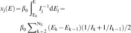
Results of second integration based on equation (5) for a CS and b A625

For metal 1, the integration will proceed from a larger E (E ₀) towards a smaller E (E _corr1) and produce negative x ₁ values from 0 (Fig. 5a), while the integration for metal 2 will proceed from a smaller E (or E ₀) to a larger E (or E _corr2) and produce positive x ₂ values from 0 (Fig. 5b). Integration ends when I _j = 0, at E _corrj.

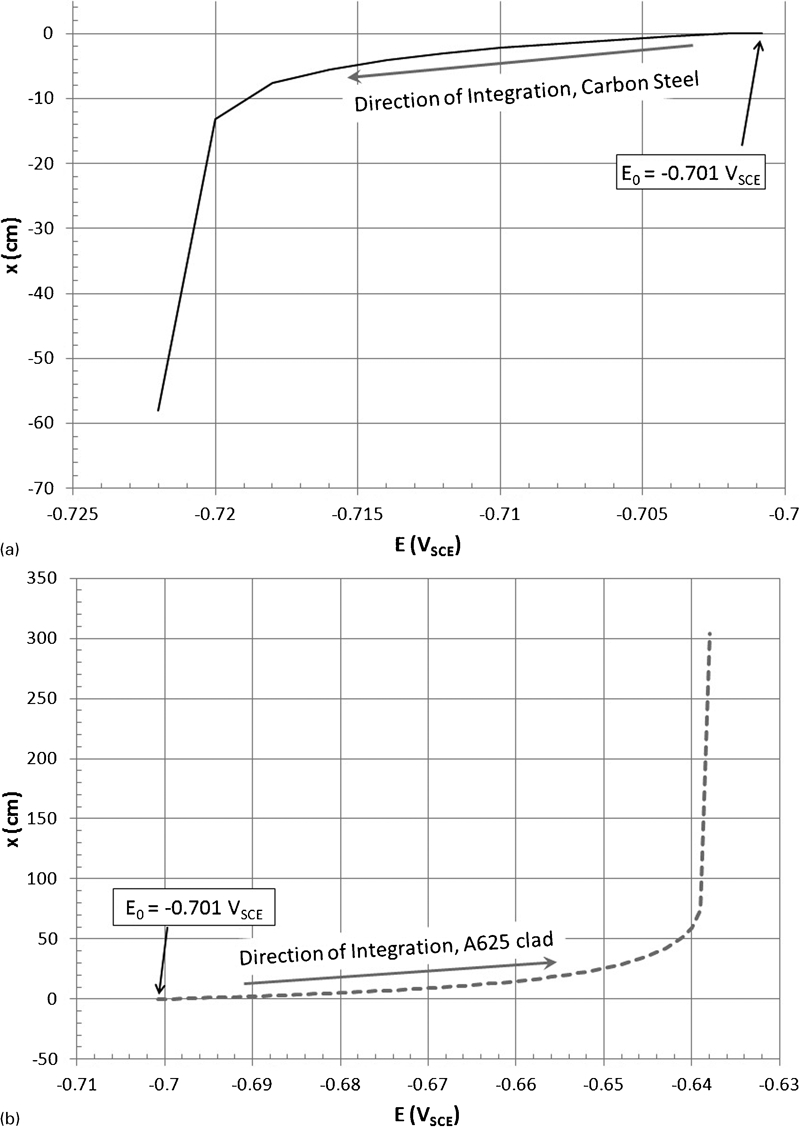
The fourth and final step is to plot E versus x for both metals on one graph. The lines will meet at x = 0, and the slopes of the lines will also match. Other curves, such as I _j versus x _j, can be plotted on a different graph and i _netj versus x _j on another graph. Examples of these plots are shown in Fig. 6 when scaling is applied in the charts following equations (2) and (2a). Such scaling plots do not vary due to the variation of pipe diameter. Shown in Fig. 6, for two other pipes with different diameters of D/4 and 4D, the scaled quantities at the same distance x from the joint shift along the curve. Relative to the quantities with pipe diameter D, the shift goes towards the left for the larger diameter and right for the smaller diameter.

Figure 6

Distributions along pipe axial direction of a potential E, b pipe cross-section current I and c current density across metal/solution boundary i _net, all in scaling plot; D is pipe inner diameter, and ρ is electrolyte resistivity

When the corrosion current density (or rate) distribution along the piping is needed, the Tafel equation for the oxidation of the active metal (steel) and the passive current density for the passive metal (A625) must be known. The results will be given in the next section.

Comparing spreadsheet method with traditional methods

Traditionally, equation (2) has been solved numerically using the polarisation data as the model input or using Tafel equations derived from the polarisation data as the model input. The use of Tafel equations requires extrapolating the Tafel slopes from the polarisation data, unable to capture the full polarisation behaviours (although in most cases sufficient). When the Tafel equations can be simplified and replaced by only the linear term of the Taylor's series expansion, an analytical solution can be obtained. Results obtained from these traditional methods will be compared with the results obtained from the spreadsheet method reported in this paper.

The numerical solution of equation (1) can be obtained using a commercial software program called COMSOL Multiphysics, version 3.5a. In the 1D numerical model, boundary conditions are set up to be zero current at each end of the long pipe. Even though the actual pipes are very long, since the current and potential rapidly level off from the joint, the modelled pipe lengths can be much smaller than the real pipe lengths (Fig. 1). For the system of concern, the length of each pipe section requires only several diameters of the pipe.

The experimental polarisation data sometimes need to be processed before they can be used as the model input. Such data are often obtained by step varying potential E to measure the current. Depending on the type of material used as the working electrode, the electrolyte composition and the experimental conditions (gas purging and temperature), the measured current can contain noise (such as titanium in sour brine), and the measured E values may not always be monotonic. For the numerical modelling, monotonic E values must be used. While not required but useful for achieving stability of the numerical modelling, the noise in current can be removed by smoothing the data.

For the polarisation data used in this work, all E values are monotonic and the current are smooth, and thus, no further treatment of this set of polarisation data is necessary. It is however worthwhile to mention that we have developed a MATLAB code that allows for automatic smoothing of the measured polarisation current and making the E values monotonic. Although this code need not be used in this work, it has found great values in other works that are being performed.

A comparison of the axial potential distribution obtained from the spreadsheet and the numerical method with direct use of the polarisation data is shown in Fig. 7. The results of the spreadsheet and numerical methods are consistent with each other, with small differences shown on the A625 section.

Figure 7

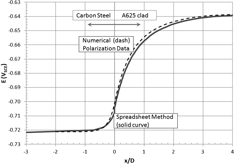
Comparison of potential distribution for spreadsheet method versus numeric method using smoothed raw data as model input

For the numerical method, the net current density i _net expressed by Tafel equations for both metals can also be used. For steel (6) where b _Fe and b _{C_Fe} are the Tafel slopes of iron oxidation and, grossly, all cathodic reactions (including acid reduction, water reduction and if present, oxygen reduction) at the steel surface respectively. E _{corr_Fe} and i _{corr_Fe} are the steel OCP and corrosion current density respectively, and they were obtained earlier from the steel polarisation curve.

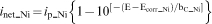
For A625, a passive alloy (7) where b _{C_Ni} is the Tafel slope of grossly all cathodic reactions at the A625 surface. E _{corr_Ni} and i _{p_Ni} are the A625 OCP and passive current density respectively, and they were obtained earlier from the A625 polarisation curve.

The Tafel slopes must be extracted by fitting the experimental data. Then, the Tafel equations (6) and (7) are supplied as model inputs for i _net to obtain the numerical solution for equation (2). The trial and error fitting of the Tafel equations to the original polarisation curves is used and shown in Fig. 8. The fit parameters are listed in Table 1. By replacing the polarisation data with the Tafel equations, COMSOL is again used to obtain the distribution of the corrosion potential along the pipes, and this distribution of corrosion potential is compared with the results from the spreadsheet method. Figure 9 shows that the Tafel equation method appears to yield results in good agreement with those from the spreadsheet method, except (again) on the steel pipe side.

Figure 8

Comparison between raw i _net data and Tafel equation fitted i _net data for CS and A625

Figure 9

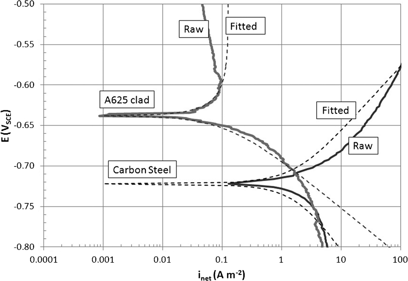
Comparison of potential distributions obtained from spreadsheet method (solid thicker curve), numerical method using Tafel equations (broken curve) and an analytical method (solid thin curve)

Table 1

Tafel equation and i _net fitting parameters

Data for steel			Data for A625
Name	Value	Units	Name	Value	Units
E _{corr_Fe}	−0·722	V(SCE)	E _{corr_Ni}	−0·638	V(SCE)
i _{corr_Fe}	1·53	A m⁻²	i _{p_Ni}	0·127	A m⁻²
R _{p_Fe}	0·0126	Ω m²	R _{p_Ni}	0·205	Ω m²
b _{C_Fe}	0·1	V(SCE)	b _{C_Ni}	0·06	V(SCE)
b _Fe	0·08	V(SCE)

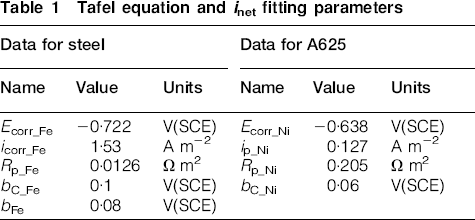
An analytical solution of equation (2) is available only when the Tafel equations can be approximated by the linear term of a Taylor's series expansion. Equations (6) and (7) respectively become (8) and (9) where R _{p_Fe} and R _{p_Ni} are the linear polarisation resistances of the two metals respectively. These values were measured experimentally from independent linear polarisation resistance tests and are also listed in Table 1. They are related to the Tafel slopes and corrosion current density at the OCP by R _{p_Fe} = B _Fe/i _{corr_Fe}, with B _Fe = 2·303b _Feb _{C_Fe}/(b _Fe+b _{C_Fe}), and by R _{p_Ni} = B _Ni/i _{p_Ni}, with B _Ni = 2·303/b _{C_Ni}.

With these approximations, the analytical solution of equation (2) is for the steel pipe section (10) and, for the A625 section (11) where E _Ni–Fe = α _FeE _{corr_Ni}+α _NiE _{corr_Fe}, E _Δ = E _{corr_Ni}−E _{corr_Fe}, γ = (R _{p_Ni}/R _{p_Fe})^1/2, α _Fe = 1/(1−γ) α _Ni = γα _Fe, λ _Ni = [4ρ/(R _{p_Ni}D)]^1/2 and λ _Fe = γλ _Ni.

In Fig. 9, the analytical results obtained from equations (10) and (11) are also shown, for comparison. Far away from the joints, all model results converge, as expected, where the corrosion potential must approach the OCP. However, the analytical solution is not consistent with the spreadsheet results, suggesting that the analytical method may yield large errors when used for prediction of the galvanic effects. The error can grow larger when the two pipe metals have a larger difference in their OCPs. In such a case, the linear approximation of the Tafel equations becomes much less valid.

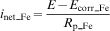
When the potential distribution in the piping is known, as shown in Fig. 9, regardless of the method used, the corrosion current density (or rate) distribution can be easily obtained from just the Tafel equation of metal oxidation, using the first term on the right hand side of equation (6) for steel and that of equation (7) for A625. The corrosion current density distributions obtained from the spreadsheet method and the analytical method are given in Fig. 10, where the differences in i _corr result from the differences in potentials obtained. Note that the same calculation can be made for the two numerical methods, although the results are not shown.

Figure 10

Comparison of corrosion current density distributions obtained from spreadsheet method and analytical method

Merits and limitations of spreadsheet method

The spreadsheet method is shown to give consistent results from the numerical method by directly using polarisation data as the model input. These methods give more robust results than the numerical method with use of Tafel equations or analytical expressions. The latter two methods use only a portion of the polarisation data to obtain results. The advantage of the spreadsheet method over the numerical methods is that it can provide access to a significantly wider range of users while giving robust results. The limitation of the spreadsheet method is that it cannot be applied to three coupling metals when one metal has a strong galvanic effect on the other two metals. It is also inapplicable to two shorter coupling pipes when the galvanic effect does not die out at the pipe ends and the potentials at the pipe ends are unknown.

For the system of interest, the Wagner polarisation parameter is calculated to be W = 0·063 m for steel and W = 1·03 m for A625. Because D/W is <4 for both metals, the 1D simulation of the piping galvanic system is valid.

In the first step of the four-step spreadsheet method, the OCP for each metal E _corr is often measured before conducting the polarisation scans, and it may be different from the corrosion potential E _corr at the smallest |i _net| on the polarisation curve. If the measured E _corr's of the two metals fall within the range of the E _corr's determined from the polarisation curves, the measured E _corr's should be used. Otherwise, between the measured E _corr and the E _corr determined from the polarisation curve, the more negative E _corr of the noble metal and the more positive E _corr of the active metal should be used.

Conclusions

An explicit four-step procedure was developed and reported that requires only the use of a spreadsheet to obtain the axial potential and current distributions of two jointed pipes of dissimilar metals. An example is provided to demonstrate how this spreadsheet method can be implemented step by step.

A great advantage of this tool is that experience in numerical simulation is not needed for one to perform the prediction. Results obtained from this spreadsheet tool are consistent with those from the numerical method by directly using polarisation data as the model input. Both methods yield more robust results than the numerical method with use of Tafel equations or analytical expressions. The latter two methods can use only a portion of the polarisation data.

A scaling method is provided that allows for charts generated from one given pipe diameter to be extended to other sizes of pipe diameter without need for additional calculations.

The limitation of the spreadsheet method is that it cannot be applied to three coupling metals when one metal has a strong galvanic effect on both other two metals. This method also does not apply to the condition with two shorter coupled pipes where the galvanic effect cannot die out at the pipe ends and the potentials at the pipe ends are unknown.

Footnotes

Acknowledgements

This work resulted from thoughts of the authors and the collaborations with several people in multiple projects. A. L. Nordquist is a student intern from the University of Texas at San Antonio, San Antonio, TX, USA.

References

Vera

Hernández

Scott

Moghissi

: ‘Predicting galvanic CO₂ corrosion in oil and gas production systems’ Proc. Conf. Corrosion 2008, Houston, TX, USA, March 2008, NACE International, Paper 08539.

Gui

Hill

Kang

Joia

: ‘Inhibition of galvanic corrosion of carbon steel and nickel alloy in oil and gas production applications’ Proc. Conf. Corrosion 2010, Houston, TX, USA, March 2010, NACE International, Paper 10333.

Kang

Joia

Augusto

Magalhaes

: ‘Evaluation of inhibitor for galvanic corrosion of nickel alloy and CS1018 couple under flowing conditions’ Proc. Conf. Corrosion 2011, Houston, TX, USA, March 2011, NACE International, Paper 11270.

R. W. Schutz, C. F. Baxter and C. S. Caldwell, ‘Effect of sour brine environment on the S–N fatigue life of grade 29 titanium pipe welds’, Proc. Conf. Corrosion 2010, Houston, TX, USA, March 2010, NACE International, Paper 10313.

Schutz

: ‘Guidelines for successful integration of titanium alloy components into subsea production systems’ Proc. Conf. Corrosion 2001, Houston, TX, USA, March 2001, NACE International, Paper 01003.

Venkamraman

Goolsby

: ‘Hydrogen embrittlement in titanium alloys from cathodic polarization in offshore environments, and its mitigation’ Proc. Conf. Corrosion 1996, Houston, TX, USA, March 1996, NACE International, Paper 96554.

Gartland

Bjornk

Schuk

: ‘Prevention of hydrogen damage of offshore titanium alloy components by cathodic protection systems’ Proc. Conf. Corrosion 1997, Houston, TX, USA, March 1997, NACE International, Paper 97477.

Hara

Asahi

Kaneta

: ‘Galvanic corrosion in oil and gas environments’ Proc. Conf. Corrosion 1996, Houston, TX, USA, March 1996, NACE International, Paper 96063.

Gartland

Johnsen

Valen

Rogne

Drugli

: ‘How to prevent galvanic corrosion in seawater piping systems’ Proc. Conf. Corrosion 1996, Houston, TX, USA, March 1996, NACE International, Paper 96496.

10.

Holser

Prentice

Pond

Guanti

: Corrosion 1992 48 332–340.

11.

Astley

: Corros. Sci. 1983 23 801–832.

12.

Shifler

Melton

: ‘Control measures to mitigate galvanic corrosion’ Proc. Conf. Corrosion 1999, Houston, TX, USA, March 1999, NACE International, Paper 99319.

13.

Wagner

: J. Electrochem. Soc. 1951 98 116.

14.

Song

: Corros. Sci. 2010 52 455–480.

15.

Frumkin

: Zh. Fiz. Khim. 1949 23 1477.

16.

Song

: Corros. Sci. 2012 57 279–287.

17.

Turnbull

Thomas

JGN

: J. Electrochem. Soc. 1982 129, 1412-1422.

18.

Vera

Shirah

Song

: ‘Laboratory evaluation of galvanic CO₂ corrosion and inhibition of carbon steel piping partially clad with alloy 625’ Proc. Conf. Corrosion 2009, Houston, TX, USA, March 2009, NACE International, Paper 09566.