
Abstract
A simple experimental method is suggested to characterise the electrode reactions of metals in an electrolytic solution in order to plot the actual corrosion state of metals in the E–pH plane. The present approach is based on measurement of the composition (in particular the pH) of the near surface layer and not on the bulk solution by application of a partition cell and simultaneous measurement of the current and application of a new approach to separate the anodic (dissolution) and cathodic currents. The resistance of the metal to corrosion is deduced from the actual dissolution current. A corrosion diagram of several metals and of the Fe–Cr binary alloy system is constructed to illustrate the potential applications of the method.
Keywords
Introduction
Pourbaix paved the way for the thermodynamic calculations of metal corrosion diagrams.1 He also provided simplified versions of corrosion diagrams for engineering application. These simplified diagrams delineate the boundaries of the potential E for three corrosion states: immunity, passivation (a layer of oxide is formed on the surface of the metal; the protective capacity of the layer remained undefined) and corrosion; the rate of metal corrosion was not determined. However, the corrosion diagrams proved unsatisfying for practical application, as the predictions derived from the diagrams do not conform with actual behaviour of the corresponding metals and solutions. Evans2 attributed this failure to conform with the experiment to certain kinetic features of the electrode reactions. In particular, it is understood that the predicted existence of oxide does not guarantee a stable passivation layer.
The corrosion behaviour of a metal in a solution is characterised by potentiodynamic polarisation, measurement of galvanic current or spectroscopy of the electrochemical impedance (e.g. Ref. 3). It is already well recognised that all the important information about the electrode reactions should be obtained by conducting measurements in the layer of solution immediately adjacent to the electrode. Electrode reactions remove necessary components from the solution and discharge their products in the nearest layer of the solution. Hence, the composition of the layer beside the electrode will vary in strict accordance with the electrode reactions. Since this concentration layer is situated between the surface of the metal and the remainder of the solution, it may be termed the ‘buffer layer’. Under stationary conditions (after prolonged exposure), the buffer layer will have a certain composition. When the external polarisation changes, the electrode reactions may change and the composition of the buffer layer will change accordingly; however, the rest of the solution will remain practically unaffected.
A variety of approaches have been adopted to study the buffer layer. Scanning reference electrode was frequently used to directly measure pH and surface potential distribution near the metal surface in bulk and in a thin layer of electrolyte (Refs. 4 and 5 and references therein). Turnbull6 reviewed the methods and results of measurements in confined conditions of corrosion with limited exchange of the solution, which are encountered in pittings, cavities, crevices or cracks where the entire volume of the separated solution is in essence the buffer layer. He also describes the use of a two-compartment cell to investigate the pH in the solution in the vicinity of the metal surface (at a distance of ∼0·5 mm) in a crevice using an Sb microelectrode in a glass capillary tube. Iridium and tungsten electrodes have also been used to measure local pH.4 More recently, flowing electrolyte techniques have been devised. A scanning droplet cell was used to measure potentials and impedance at the level of grain boundaries.7 A scanning microflow cell was used to maintain a stream of electrolyte on a metal surface and harvest the drained electrolyte for spectroscopic analysis.8 It allowed following the evolution of potential, current and metal dissolution with the time of the corrosion process.
In order to approximate the actual composition of the solution with which the metal interacts under stable conditions, we suggest to employ a partition cell that makes it easy to measure and analyse the buffer layer, does not call for special equipment, allows the use of standard electrodes and produces stable results (Fig. 1). Kuhn and Chan9 emphasised the importance of measuring the pH near the surface during electrochemical reactions. Thus, in the following, we choose the pH as the key characteristic of the buffer layer since most electrode reactions affect the solution pH. To obtain information about both the electrode reactions that take place on the metal surface and the corrosive state of the metal, the procedure is as follows:
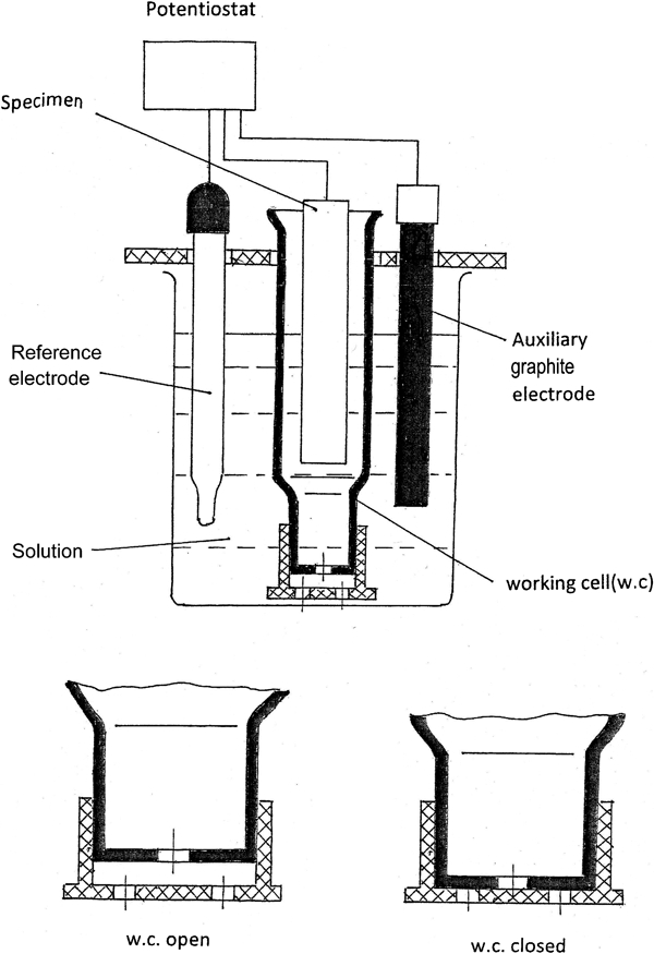
Compartmentalised electrochemical cell; partition is kept open under conditions of operation and closed during measurements
use a partition electrochemical cell containing the metal and the solution as model of the buffer layer of the solution
apply the selected electrode potentials (from an external source of potentials) in a potentiostatic regimen of polarisation
after a certain exposure time at each potential, measure the pH of the solution in the working chamber or determine the concentration of certain ions by chemical analytic methods
using the results of the measurements, construct a polarisation diagram for E versus pH (or E versus the concentration C of certain ions).
To interpret the changes in the pH of the solution, the experimental E–pH diagrams and the theoretical Pourbaix's diagrams for the corresponding pure metals are superimposed. Using Pourbaix diagrams, it is necessary to take into account the potentials of the metal and the corresponding real concentrations of the buffer layer of the solution with which the metal interacts and not the whole initial solution. The superposition revealed near or complete matching between the boundaries of phase transitions on the Pourbaix diagrams and the kinks in the E–pH curves.10 The coincidence of the lines helps to interpret the E versus pH curve, namely, to attribute the form of the line to the corresponding electrode reaction. We thus constructed diagrams of the corrosion regions of the type of Pourbaix diagrams except for the new diagrams being constructed according to the composition of the buffer layer for several metals in a range of pH values.11 These diagrams show the corrosion states of the metals, but they are still lacking an essential characteristic: a measure of the resistance to corrosion and of the potency of passivation.
Therefore, in addition to the measurement of the E–pH relation, it is necessary to measure also the metal dissolution current at each polarisation potential in order to elucidate the actual corrosive state of the metal. Thus, while passivation is determined by the thermodynamic stability of the metal oxide in the approach of Pourbaix, we determine the passivation by the actual vanishing of the dissolution current. Only vanishing of the current indicates the existence and the stability of the oxide.
The initial dissolution potentials and the corrosion potentials of many metals lie in the zone of cathodic depolarisation in the E–I diagram. The cathodic line represents the sum (cathodic and anodic) current; therefore, it is necessary to separate from the line of anodic (dissolution) current. In the present work, the cathodic lines of the current in the cathode–anode transition zone were studied for a number of metals to enable the separation of the dissolution current and the identification of the electrode reactions. Then, the approach was extended to the Cr–Fe alloys in a 3%NaCl solution, and a corrosion diagram was constructed for the Fe–Cr binary system.
Materials and methods
The experiments were conducted in a compartmentalised electrochemical cell (Fig. 1) simulating the buffer layer of the solution. Polarisation diagrams in terms of E–I and E–pH for the buffer solution under synchronous measurement of I and pH were constructed for a number of metals (Pt, Zn, Cu, alloys 2024 and 304, Fe, Cr and a series of alloys in the Fe–Cr system). Pt was chosen to represent an insoluble metal. To ensure a nearly stationary state of the buffer solution and of the current in the cell, we performed all measurements following a prolonged exposure (4 h) to the potential. The stationary metal corrosion potentials E cor were determined after 24 h of residence in the solution. All the reported potentials are expressed relative to the hydrogen standard electrode.
The volume of cell in which the tested electrode was placed measured 12 cm3. The samples were in the form of cylinders 8 mm in diameter; the Pt sample was in the form of a cylindrical spiral. The corrosive solution consisted of 3%NaCl, pH 6·5. The area of sample immersed in the solution was 12 cm2.
The cell used to model the buffer layer of the solution represents an approximation to the real state of the buffer layer and introduces a certain measure of error. The principal error is the jump of the ion concentration in the solution on the two sides of the partition and, correspondingly, the formation of a liquid boundary potential. This results in the real potential of the metal deviating from the potential applied by the potentiostat. This deviation is most significant for large concentration jumps. For a neutral chloride solution and a negative polarisation of −2·0 V applied to Fe (i.e. maximum concentration differences), computation by Henderson's method12 gives a potential drop of ξd = 0·1 V at the diaphragm for the maximum concentration. For small currents and for potentials close to the potential of a standard hydrogen electrode in a neutral solution, the correspondingly ξd tend to 0. In this study, we examined minimal currents at the stage of cathodic–anodic transition, and therefore, any errors introduced by the diaphragm were minimal.
Results and discussion
General observations in cathodic region
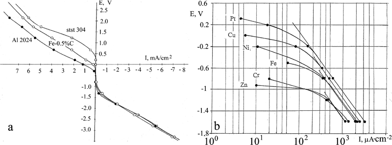
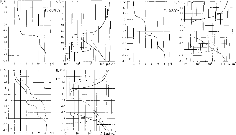
E–pH and E–I polarisation diagrams in the potential interval from −1·8 to +2·2 V corresponding to the interval of potentials in Pourbaix diagrams were constructed based on the results of measurements in a partitioned cell for the selected metals in a neutral solution of 3%NaCl. We start with the characteristic features of the cathodic region of negative potentials. At high currents, a linear relation between current and potential prevails (Fig. 2a). At the potential E = −1·5 to −1·6, a transition occurs to a low current region, I = 1 to 103 μA cm−2. Plotting the data in this region in a logarithmic scale (Fig. 2b) reveals that all the studied metals form straight parallel lines indicating that the current vary exponentially with the potential. The common behaviour of all the metals indicates that a similar surface reaction (hydrogen reduction) with identical solution including the buffer layer takes place without an active participation of the metal surface. At higher potentials, each line deviates from a straight line in the E–I diagram at a characteristic potential listed in Table 1. The straight current line segment of platinum reaches E = −0·3 V. Since Pt is insoluble, we find that the exponential law of hydrogen depolarisation holds at least up to E = −0·3 V. The divergence of the lines of the different metals reflects beginning of metal dissolution. This is also confirmed by the E–pH diagrams: at electrode potentials E = −1·8, the pH of buffer solution was maintained at ∼12 for all the metals, making evident the active discharge of hydrogen ions (Figs. 3d, 4b, 5b, 6b, 7b and 8b, d, f, h, j, l, n). The E–pH polarisation diagram of the buffer layer shows a deflection in the direction of lower pH values near the potential where the current lines begin to deviate from the straight line (Figs. 3a, 4a, 5a, 6a, 7a and 8a, c, e, g, i, k, m). This is due to the sum of two processes: the formation of a hydroxide of the dissolved metal and the gradual cease of the reduction in hydrogen (hydrogen depolarisation).
E–I polarisation diagrams; potentials are reported relative to hydrogen standard electrodes
Schematic E–pH and E–I polarisation diagrams
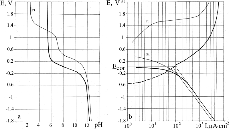
E–pH and E–I polarisation diagrams for Zn
E–pH and E–I polarisation diagrams for Cu
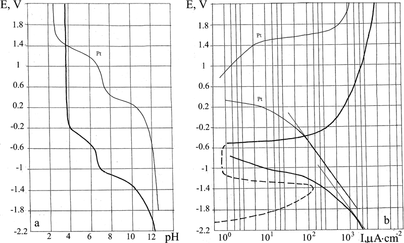
E–pH and E–I polarisation diagrams for Al alloy 2024
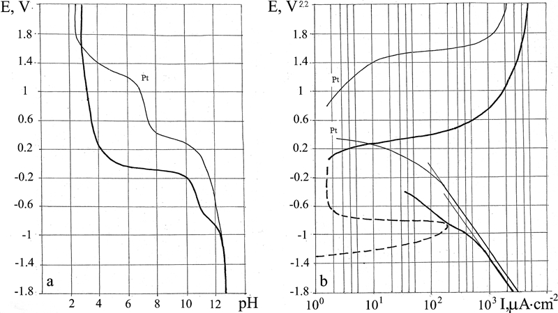
E–pH and E–I polarisation diagrams for alloy 304
E–pH and E–I polarisation diagrams
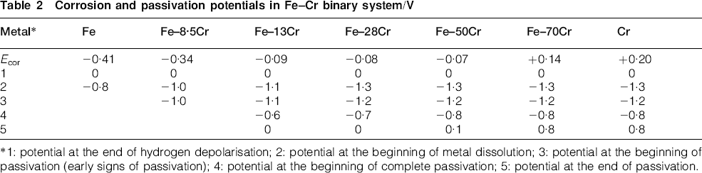
Potentials where metal current lines begin to deviate from straight line
Non-passivating metals
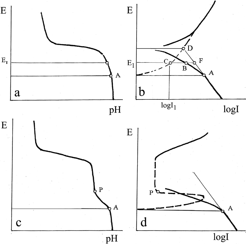
The beginnings of metal dissolution potentials are practically identical with the potentials marking the start of dissolution of the respective metal on the Pourbaix diagrams at a solution pH of 12. The magnitude of the divergence of the current line for a given metal from the straight Pt line may be used to obtain an estimate of the metal dissolution current. Figure 3 shows schematic curves for a non-passivating metal (Fig. 3a and b) and a passivating metal (Fig. 3c and d). The dotted lines in the diagram indicate the calculated metal dissolution current lines. The dissolution starts at point A, where the cathodic current line diverges from the initial straight line. The dissolution current in the region of cathodic polarisation at the potential E 1 is given by BF = E 1C, and the cathodic current is E 1F. The calculated dissolution current can be verified by the current at the corrosion potential E cor on the E–I diagram. By the potential of corrosion Ecor the condition of equality of the anodic and cathodic currents must be fulfilled. In Fig. 3b this condition is satisfied at the intersection of the straight line AD and the dotted line at a potential Ecor - this is point D (with actual measurements - close to D). So that D is the control point.
Passivating metals
A distinguishing feature in the cathodic zone of the E–pH diagrams of passivating metals is the presence of a double kink corresponding to cathodic depolarisation before and after the formation of the passivating film (Fig. 3c).
In the beginning of segment AP on the E–I line (Fig. 3d), the dissolution current is calculated as for non-passivating metals. At point P, the passivating film is fully formed, the metal dissolution nearly ceases and the cathodic depolarisation declines sharply.
It is found that the passivation current is approximately equal to the minimal current at the line of active anodic solution. (Fig. 3d).
Next, the low current cathodic region and the anodic regions will be examined for two non-passivating metals and two passivating metals in a 3%NaCl solution in comparison with Pt. This comparison allows the identification of the dissolution current of the reactive metals.
Examples
Zn
Figure 4 shows E–pH and E–log I polarisation diagrams of Zn and Pt for comparison. The point of divergence of the cathodic line of current from the initial straight line corresponds to the potential of the start of metal dissolution (E = −1·3 V). The metal dissolution current line (dotted line in Fig. 4b) up to its meeting with the anodic current is constructed using the difference between the cathodic line of current and the initial straight line.
The straight line of cathodic current at the stationary corrosion potential (E cor = −0·81 V) gives the value of the hydrogen depolarisation current at the corrosion potential. The anodic dissolution (broken) line intersects the straight line, indicating the same magnitude of the anodic current. This confirms that the hydrogen depolarisation proceeds practically unhindered even when dissolution of the metal takes place and that the Zn(OH)2 formed during such dissolution does not constitute an appreciable obstacle to either metal dissolution or hydrogen depolarisation; therefore, the surface of the Zn is not passivated.
Cu
The types of E–pH and E–I diagrams obtained for Cu (Fig. 5) confirm that it is a non-passivating metal. Dissolution begins at E = −0·5 V. In the potential interval −0·5 to −0·3 V, the metal dissolution current is calculated according to the difference between the cathodic line and the initial straight line; at higher potentials, the metal dissolution line joins the anodic line.
Al alloy 2024
Judging by the characteristic form of the E–pH polarisation diagram (Fig. 6) of the buffer layer, alloy 2024 may be classed among the passivating metals. According to the E–I diagram, dissolution of the metal begins at E = −2 V. A comparative study of the two diagrams indicates that the metal is passive starting from potentials E = −1·4 V and higher. The stationary corrosion potential E cor = −0·49 V lies dangerously close to the zone of active metal dissolution (i.e. the reserve of passivity is not sufficiently large to afford protection).
Stainless steel 304
The types of E–pH and E–log I diagrams obtained for alloy 304 (Fig. 7) correspond to a passive metal. The corrosion behaviour of this alloy is similar to that of Cr (Fig. 8m and n), except that the current passivation interval is smaller for this alloy (E = −0·8 to +0·2 V) than for Cr (E = −1·0 to +0·8 V). The broken line on the E–log I diagram shows the metal dissolution current. The stationary corrosion potential E cor = +0·055 V lies in the zone of passive current quite far from the zone of active dissolution.
Fe–Cr binary system
The present approach to characterise the corrosion of metals has been extended to a systematic examination of the evolution of the electrochemical behaviour in alloy systems. Comparing the behaviour at different compositions may be important from both basic science and engineering selection of materials. The most interesting system to study is the Fe–Cr binary system due to the passivation properties that the Cr imparts on steels. We begin with the behaviour of the pure elements.
Fe
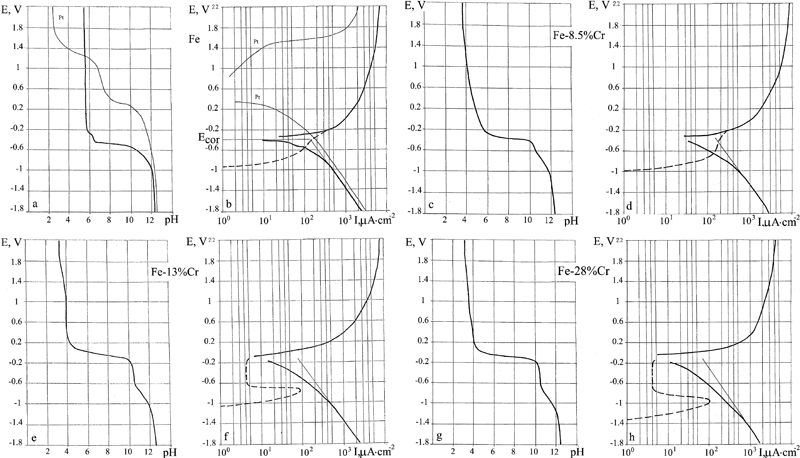
As shown by the E–log I diagram for Fe (Fig. 8a and b), beginning of Fe dissolution takes place at E = −0·8 V. This is also confirmed by the E–pH diagram of the buffer layer: starting from the potential E = −0·8 V, the pH is seen to decline due to formation of Fe(OH)2 in the solution. The measured stationary corrosion potential E cor = −410 mV.
The anomalous deflection of the current line and the pH line on the E–log I and E–pH diagrams, at potentials E from −0. 5 to −0·4 V, is probably due to the change in valence of the dissolved ions, namely, Fe2+→Fe3+. On the theoretical Pourbaix diagram for Fe,1 this is where the boundary between the formation of Fe(OH)2 and of Fe(OH)3 lies. The calculated metal dissolution line (dotted line in Fig. 8b) changes smoothly into the anodic current line. The difference between the dissolution current line and the straight line of the cathodic current at the stationary corrosion potential demonstrates that hydrogen depolarisation proceeds even after dissolution of the metal starts and that the Fe(OH)2 formed during iron dissolution does not obstruct either metal dissolution or hydrogen depolarisation.
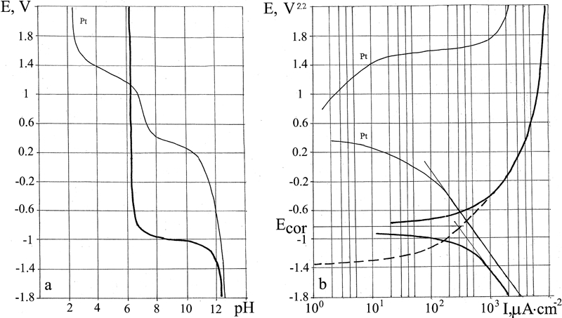
Cr
The E–pH polarisation diagram for Cr (Fig. 8m and n) shows three kinks. The first kink above E = −1·3 V is due to the sum of gradual cease of the hydrogen depolarisation and dissolution of metal that forms chromium hydroxide. The second kink represents the cease of the hydrogen depolarisation. The third kink at 1 V is due to the breakup of the passivation and the beginning of active metal dissolution that induces acidification of the buffer layer. The stationary corrosion potential E cor = +0·2 V lies in the zone of passive metal dissolution.
In the interval from E = −1·4 to 1·0 V, the metal dissolution current is calculated using the difference between the cathodic current lines and the initial straight line. We can assume that the metal dissolution current is equal to the minimum initial current on the anodic line.
The metals and alloys examined above, i.e. Zn, Cu, Al alloy 2024, stainless steel 304, Fe and Cr, have been thoroughly studied in practical applications, and a great deal is known about their corrosion properties. In particular, the potentials at which metal dissolution begins1 and their different tendencies to passivation in chloride solution are well known.13 In general, the foregoing analysis of the E–pH and E–I diagrams conforms with the known data.
Fe–Cr Binary system
In Fig. 8, we constructed the E–pH and E–I diagrams in the range of small metal dissolution currents (the cathode–anode transition) for a series of alloys in the binary system with the aim of establishing the boundaries of passivation. The following alloys were prepared and tested: Fe, Fe–8·5Cr, Fe–13Cr, Fe–28Cr, Fe–50Cr, Fe–70Cr and Cr. To construct a general corrosion diagram for Fe–Cr using the E–pH and E–I diagrams of the individual metals, the potentials of several characteristic points are listed in Table 2: beginning and end of hydrogen depolarisation and metal dissolution, and beginning and end of the passivation potentials.
Corrosion and passivation potentials in Fe–Cr binary system/V
*1: potential at the end of hydrogen depolarisation; 2: potential at the beginning of metal dissolution; 3: potential at the beginning of passivation (early signs of passivation); 4: potential at the beginning of complete passivation; 5: potential at the end of passivation.
In constructing the corrosion diagram for the binary system, the main emphasis was on determining the boundaries of the states of corrosion of the alloys (Fig. 9). The line of stationary corrosion potentials E cor on the diagram served as orientation in evaluating the position of the boundary between passivation and corrosion. The diagram reveals the increase in corrosion resistance with rising content of Cr in two jumps: at the celebrated 13Cr jump and at ∼60Cr a second jump. The alloys between 13 and 70%Cr are close to the passivation boundary; therefore, their passivation is relatively unstable.
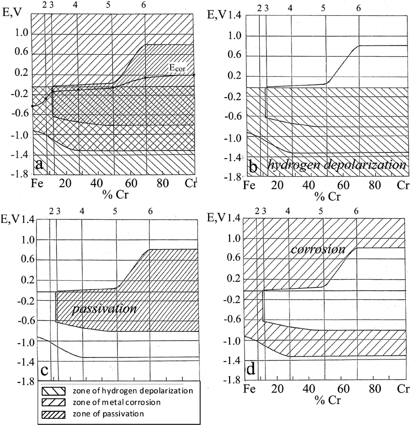
Diagram showing corrosion resistance in Fe–Cr binary system; upper boundary of each figure indicates compositions of five alloys that were tested (2: Fe–8·5Cr alloy; 3: Fe–13Cr alloy; 4: Fe–28Cr alloy; 5: Fe–50Cr alloy; 6: Fe–70Cr alloy)
These diagrams have been prepared assuming stagnant (no flow) conditions. However, there will probably be changes in a moving solution, for example, in altering the formation of the normal pH buffer layer and on the electrochemical double layer. It seems that we can expect that (i) the intensity of depolarisation will increase at either the cathodic or the anodic, or on both reactions and (ii) the corrosion potential of the metal will change to accommodate the kinetic changes in the form of the polarisation curve.
Conclusions
During the interaction between the metal and the electrolytic solution, a buffer layer is formed near the metal surface. The composition of the buffer layer changes in accordance with changes in the potential of the polarised metal and is important for understanding the metal corrosion process. The theoretical basis for constructing diagrams of metal corrosion in an interval of potentials that was provided by Pourbaix's thermodynamic diagrams is adjusted here for the buffer layer where the actual electrode reactions take place.
The state of corrosion or the electrode reactions of metals in intervals of potentials and the metal dissolution currents were established by simultaneous measurements of the pH of the buffer layer and the total current.
The pattern of the E–pH curve enables to distinguish the potential intervals of hydrogen polarisation, start of metal dissolution, passivation limits and transition between oxidation states of the metal. The pattern of the E–I lines allowed to separate the anodic and cathodic currents for several metals and alloys by comparison with Pt. A corrosion diagram for the whole Fe–Cr binary system was constructed and revealed two transitions in the resistance to corrosion.