An assessment of climate change effects on atmospheric corrosion rates of steel structures

Abstract

This paper presents a discussion on assessing the potential impacts of climate change on the atmospheric corrosion rates of exposed steel structures. The effects on atmospheric corrosion due to changes in the environmental temperature, carbon dioxide, relative humidity, wind, rainfall and pollution are considered. The limitations and complexities of these assessments are discussed. To demonstrate the use and limitations of this science to evaluate effects related to climate change, a model developed in Australia to predict corrosion is combined with climate change models to project the change in the corrosion rates of steel components and protective zinc coatings in constructions. The method is applied to constructions located along the coastal areas of two Australian cities: Melbourne and Brisbane. These assessments are made using the A1FI scenario, the highest emission scenario defined by the Intergovernmental Panel on Climate Change, applied to nine general circulation models. The projected changes in corrosion rates were found to be an increase of ∼14% for both zinc and steel in Brisbane and a decrease of ∼14% for steel and 9% for zinc in Melbourne. It was also found that the uncertainties associated with the climate change models were small compared to those involved in modelling corrosion for engineering purposes.

Keywords

Galvanised steel Zinc coating Atmospheric corrosion Climate change Emission scenario Airborne salinity

Introduction

Steel is the most commonly used material for a wide range of infrastructure components and industrial equipment. It is often employed in exposed conditions in coastal areas and/or highly polluted industrial areas, both areas where unfortunately the atmospheric corrosion is of high concern. Koch et al.1 reported that corrosion costs in the United States were about US$137·9 billion per year for 26 industry sectors and extrapolated to US$276 billion per year (3·14% of gross domestic product) for the entire US industry. In Australia, it was estimated that corrosion may have cost up to $32 billion per annum, which means more than $1500 for every person in Australia each year.2 As a mean of protection from corrosion, a zinc coating is often used on the surface of structural steel. The zinc coating (galvanising) industry for steel construction is large, consuming about half of the zinc production of the world.

Projected future climate changes will affect the extent of atmospheric corrosion, and it is important to assess the potential magnitude of these changes. Recently, Cole and Paterson3 and Roberge4 have reviewed and discussed possible impacts that climate change may have on the corrosion. It was argued that it is currently not possible or very difficult to quantify the effects of climate change on atmospheric corrosion. The arguments are based on the following: the climate change models are not clear on predictions of aerosol production and the movement of various airborne corrosive agents,3 and it is unclear as to how the world economy will evolve in the future.5 However, it is obvious that for future planning purposes, there is benefit to be obtained in assessing the magnitudes and uncertainties associated with corrosion estimates related to the use of climate change projection models.

Some work has been reported on the impact of climate change on corrosion of steel reinforcement in concrete structures (e.g. Refs. 6-8). However, this paper is probably the first to attempt to quantify climate change impacts on the atmospheric corrosion of steel structures in specific locations.

The following is a review on some significant features of atmospheric corrosion.

Review of factors related to atmospheric corrosion

Overview

The atmospheric corrosion of steel components and zinc coatings has been an active research field for several decades. It encompasses a wide range of industrial and domestic steel structural components in constructions that are fully exposed to weather and thus subjected to corrosion. Various studies have been conducted, mostly by laboratory experiments and/or field monitoring. There is generally a consensus9 ^– 11 that long term atmospheric corrosion of metal is described by the following equation (1) where c _atm is the atmospheric corrosion depth (in μm) after t years in service, c ₀ (μm) is the corrosion depth at the end of the first year, t is the duration in service (in years) and n is a power factor <1·0, giving the generic corrosion curve with time as shown in Fig. 1. Since the corrosion rate at any given time is proportional to c ₀, for descriptive convenience, we will refer to c ₀ as the ‘corrosion rate parameter’.

Figure 1

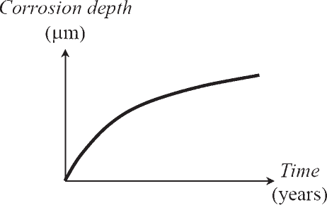
Progress of atmospheric corrosion (equation (1))

It should be noted that an alternative and rather more sophisticated concept of atmospheric corrosion in marine environments has been investigated by Melchers.12,13 For this model, he proposes several phases for the progression of corrosion, each one with its own mechanism. There is no doubt that this model is an improvement on existing models in terms of both the rationality of the corrosion mechanisms proposed and accordingly the accuracy in predicting the progress of corrosion. However, for reasons related to data availability and practical feasibility, the corrosion models considered in this paper have been chosen to relate to equation (1) above.

Many studies have been based on the use of short term measurements of corrosion to estimate the corrosion rate parameter c ₀ in equation (1) (e.g. Ref. 14) and on long term tests to estimate the power factor n (e.g. Refs. 10, 11 and 15). There has been general agreement that the corrosion rate parameter c ₀ is mainly governed by the following factors:

time of surface wetness, which is approximated as the percentage of time in a year that the metal surface is wet by a moisture layer; for Australian coastal areas, an atmospheric corrosion model16 has been fitted to the assumption that the moisture layer is formed when the relative humidity (RH) is above 80% and the temperature above 0°C

ii.

airborne salinity, in terms of chloride concentrations in the air

iii.

airborne pollution, mainly in terms of sulphide concentrations in the air.

For steel components with zinc coatings, it is assumed that the corrosion will progress successively, i.e. corrosion will first occur on the zinc coating, and then on the steel substrate after there is no zinc coating left. Corrosion of both zinc and steel in the atmosphere is a complex discontinuous electrochemical process, which happens with the presence of water on the metal surface and airborne pollutants, including sulphur dioxide in industrial areas and airborne chlorides in marine areas.

A review of the atmospheric corrosion process of zinc was provided by de la Fuente et al.11 In general, when exposed to the atmosphere with the presence of water, the reaction of zinc with atmospheric oxygen produces various corrosion products, where the most important stable carbonate is hydrozincite [Zn₅(CO₃)₂(OH)₆], which has a protective effect against further corrosion. Since the corrosion process of zinc is also remarkably slower than that of steel, the zinc coating acts as a protection layer that delays the corrosion progressing into a steel substrate, which is the part that bears the structural loads. The thickness of a zinc coating for structural steel components is usually in the range of 25-85 μm.17 For practical purposes, galvanised steel components are considered to reach the end of their service life when the zinc coating layer is fully corroded.

De la Fuente et al.15 have also provided a detailed review of the atmospheric corrosion process of steel. Oxides, hydroxides and salts (chloride or sulphate) of iron are commonly found in the corrosion products that form corrosion layers. The corrosion layers exhibit a large number of pores and microcracks that make them highly defective and permeable, and may eventually become detached when they become too thick. The corrosion layers of steel therefore practically provide little protection against further corrosion.

Effect of changes in rainfall patterns

There is a well known beneficial effect of rain in washing out the atmospheric corrosive pollutants that have settled on exposed surfaces, thus reducing the corrosion rate.18 The projection for future climate is that rainfall will occur in higher intensity falls but with reduced frequency, i.e. the cleansing effects may be reduced. In a sophisticated model, Cole and Paterson3 introduced the concept of cutoff rainfall, which is the minimum rainfall required to clean a surface. The extent of the washing effect of a rain event is then estimated depending on its intensity relative to the cutoff rainfall.

Effect of changes in RH

Apart from affecting the time of surface wetness mentioned in section on ‘Overview’, increases in RH would increase the size of surf produced aerosols and thus the salt deposit, especially in marine areas.3 However, this effect would not be significant for Australia, where RH is projected to decrease over most of the country.19

Effect of temperature

The effect of temperature on atmospheric corrosion is complex. Atmospheric corrosion is an electrochemical process. In theory, the corrosion rate is therefore dependent on ambient temperature. The dependence follows the Arrhenius law (2) where c ₀ is corrosion rate parameter, α is a frequency factor, K is the absolute temperature (kelvin), E _a is the activation energy and R is the Boltzmann gas constant (R = 8·31 J K⁻¹ mol⁻¹).

Based on the theoretical Arrhenius equation, it has been suggested that temperature could be an important factor in atmospheric corrosion.20 This has been reflected in a general ‘rule of thumb’ that ‘a 10°C increase in temperature will double the corrosion rate’18,21 within a normal range of ambient temperature of 20-30°C (293-303 K). With this rule, the activation energy E _a is ∼50 kJ mol⁻¹. Pacheco and Ferreira20 reported similar values of activation energy from a series of lab tests. However, it is important to note that this extent of the temperature effect on the corrosion is only valid at a constant condition22 of a very high humidity level.23

In reality, the atmospheric corrosion is a complex discontinuous electrochemical process subjected to highly variable ambient conditions, where the corrosion reaction only occurs when there is a moisture layer formed on the metal surface. For Australian conditions, metal surfaces commonly undergo daily wetting cycles.3 At night, as the ambient RH increases and temperature decreases, a moisture layer forms and then facilitates the corrosion reactions on the metal surface. At sunrise, when temperature increases and RH decreases, the moisture layer evaporates and thus the corrosion reactions halt. With such a complex condition, the effect of temperature on atmospheric corrosion in ambient condition was perceived to be secondary.3,24 This was also observed in the results of some field corrosion tests.11,20 Lindstrom et al.25 reported an interesting experimental result that in the presence of CO₂, the zinc corrosion rate did not show a dependence on temperature. Cole and Paterson3 have suggested that for practical applications ‘an increase of 2 K (from 293 to 295 K) will promote a 0·6% change in corrosion rate’.

Effect of pollution

Airborne pollution in terms of SO₂ is produced from industrial activities. Global projections for SO₂ have been provided by the Intergovernmental Panel on Climate Change (IPCC)26 with large uncertainties. On average, the IPCC projected that the global increases of SO₂ ‘are generally modest, and numerous scenarios even depict a long term decline in emissions’. Graedel and Leygraf5 established two scenarios for the projection of SO₂ emission at various regions and the whole world for consideration of atmospheric corrosion. One is for a ‘no control’ scenario where it is assumed that there are no new control measures on SO₂ emission in any region after 1990. While SO₂ emission levels of developing countries and the whole world are projected to increase, the SO₂ emission levels in developed countries were projected to decrease, as cleaner and more efficient technologies were employed. In particular, the levels of SO₂ emission in Australia were projected to reduce by half in 2100, even in the ‘no control’ scenario.

The pollution effects are usually only a minor component of corrosion in marine locations.3 Furthermore, pollution is essentially a local problem, where a simple formula for estimating the level of SO₂ based on distance to the industry zones and type of the industry proposed by Nguyen et al.16 is deemed to be appropriate for practical design and is not dependent on climate. Accordingly, the effects of airborne pollution on atmospheric corrosion in Australia need not be considered in the context of examining the impacts of climate change.

Effects of CO₂ concentration

The CO₂ concentration increase may have effects on zinc corrosion rates. A series of laboratory experiments reported by Chung et al.27 indicated that the formation of hydrozincite, which is the stable protective zinc corrosion product, is accelerated with increasing RH and CO₂ concentration, resulting in an increase in the resistance against corrosion and thereby a reduction in the corrosion progress of zinc. These experiments indicated that at high RH (95-100%), after 72 h exposure, the corrosion resistance of zinc specimens in a chamber of 1000 ppm CO₂ concentration is 20% higher than the resistance of specimens in a chamber of 350 ppm CO₂ concentration. These concentrations are quite similar to the condition of the climate change scenario A1FI, which has the highest CO₂ emission among all scenarios defined by IPCC. In this case, the CO₂ concentration is projected to increase from 350 ppm in 1990 to ∼1000 ppm in 2100.28 Increases of CO₂ concentration would reduce the corrosion rate, but it is important to note that this was an effect observed only at a very early stage of corrosion through experiments in laboratory conditions only, i.e. within a chamber at a constant high RH condition. Considering that the corrosion is a long term discontinuous process, this effect is likely to be secondary in reality and hence assumed to be negligible herein. Further research and validation to clarify this effect on steel component construction at real service conditions are required.

Method for assessment of climate change effects

In this study, an attempt was made to go as far as possible in using the available information on corrosion and climate change models to assess corrosion rates in the years up to 2100, relative to the values in 1990.

Most of the assessment was made using an Australian model for corrosion developed for engineering purposes;16 the model predicts the atmospheric corrosion rates of structural steel fasteners and related zinc coatings. It was developed using available scientific information and available field data to provide a set of simple parameters that were suitable for engineering applications.

Atmospheric corrosion is a complex process that depends on the interactions of many environmental factors. To account for these factors, the application of the Australian model requires the input of numerous parameters such as the geographical location of the structure, the distance from the coast, the coastal geometry, topographical influences, the terrain roughness, building shelter and parameters related to pollution.

In the following assessment, for clarity in presentation, pollution effects will not be considered, and only changes in the corrosion of structures located within the coastal zone, say within a distance of 1·0 km from the coast, will be evaluated. Furthermore, since these changes in corrosion rates will be evaluated as relative percentages, most of the engineering parameters mentioned in the previous paragraph remain constant, including the exact distance from coastline, and hence need not be considered. In addition, for reasons of clarity in presentation, corrosion rates at only two locations situated on the east coast of Australia will be examined; these are the cities of Melbourne and Brisbane.

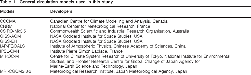
Climate change science has projected a different climate in the future with a mean global temperature increase of 4-6°C by the end of the century, leading to changes in other climate parameters and changes in intensity and frequency of weather events.19,28 For this paper, the assessments of climate change will be made using the A1FI emission scenario, the highest emission scenario defined by the IPCC, applied to the nine general circulation models (GCMs) listed in Table 1.

Table 1

General circulation models used in this study

Models	Developers
CCCMA	Canadian Centre for Climate Modelling and Analysis, Canada
CNRM	National Center for Meteorological Research, France
CSIRO-Mk3·5	Commonwealth Scientific and Industrial Research Organisation, Australia
GISS-AOM	NASA Goddard Institute for Space Studies, USA
GISS-EH	NASA Goddard Institute for Space Studies, USA
IAP-FGOALS	Institute of Atmospheric Physics, Chinese Academy of Sciences, China
IPSL-CM4	Institute Pierre Simon Laplace, France
MIROC-M	Centre for Climate System Research of University of Tokyo, National Institute for Environmental Studies, and Frontier Research Centre for Global Change of Japan Agency for Marine-Earth Science and Technology, Japan
MRI-CGCM2·3·2	Meteorological Research Institute, Japan Meteorological Agency, Japan

Models used for atmospheric corrosion

Model for corrosion due to effects of airborne salt

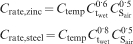
For engineering applications in Australia, Nguyen et al.16 proposed that in the absence of pollution, the mean atmospheric corrosion rate of zinc may be estimated from (3) and for steel (4) where c _0,z and c _0,s are corrosion rate parameters (μm), which are the corrosion depths (μm) of zinc and steel for the first year respectively, t _wet is the time of surface wetness (%) and S _air is the airborne salinity (mg/m²/day) (measured as a deposit on a salt candle).29 The parameter t _wet is computed as the percentage of time that the RH is >80% and the temperature is above 0°C. The general shape of the corrosion curve corresponds to equation (1) and is shown in Fig. 1.

Nguyen et al.16 presented models for estimating the parameters of equations (3) and (4) for Australia. These models were calibrated to various sources of corrosion data, including the Australian Standard AS 4312,30 various field test data31 ^– 33 and corrosion test data in South East Asia including North Australia.34 The model calibration is presented in a report by Nguyen et al.35

The effect of climate change on the parameters t _wet and S _air cannot be obtained directly from the climate change models, and so indirect methods must be used.

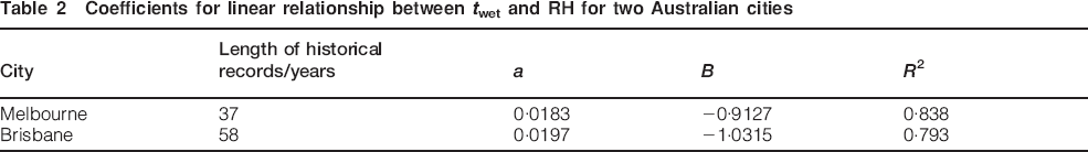
Although climate change models do not provide projected values of t _wet, they do provide projections of RH, the annual average value of RH. Historical weather data from past years have indicated that for the two target cities of Melbourne and Brisbane, these parameters have been related by (5) where the parameters a and b are given in Table 2, and the data on the parameter relationships are plotted in Fig. 2.

Figure 2

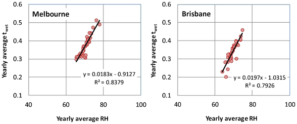
Relationships between time of wetness and yearly average of RH in Melbourne and Brisbane based on historical weather data

Table 2

Coefficients for linear relationship between t _wet and RH for two Australian cities

City	Length of historical records/years	a	B	R ²
Melbourne	37	0·0183	−0·9127	0·838
Brisbane	58	0·0197	−1·0315	0·793

For the projection of airborne salinity for the future, it will be assumed that most of this salinity is generated primarily from the action of surf and ocean waves. These sea state activities are governed by wind and fetch characteristics for a specific location. A relationship of volumetric airborne salinity S _air,vol (μg m⁻³) with mean wind speed U (m s⁻¹) was given by McKay et al.36 based on measurements as follows (6) Cole et al.37 used this relationship in the establishment of a geographic information system for the prediction of airborne salinity based on wind and fetch characteristics at any location in Australia, and produced an Australia wide map of corrosivity.38 The simplified model for estimating airborne salinity in five Australian coastal zones, presented by Nguyen et al.,16 was developed based on this prediction framework.

The climate change projections provide estimates of likely changes in mean wind speed,19 and using equation (6), these changes can be used to estimate changes of volumetric airborne salinity S _air,vol.

Model for corrosion due to effect of temperature

As noted previously in the section on ‘Effect of temperature’, Cole and Paterson3 have suggested that ‘an increase of 2 K (from 293 to 295 K) will promote a 0·6% change in corrosion rate’. Fitting this assumption to equation (2), the increase in corrosion rate with temperature can be expressed as (7) where and are the corrosion rates at absolute temperature T ₁ and T ₂ respectively. Although the effect of changes in temperature is expected to be only a minor secondary effect on corrosion rates, the temperature effect predicted by equation (7) is simple to evaluate and so will be considered in this study.

Climate change models used

As mentioned previously, the climate change impact assessment is carried out considering the A1FI emission scenario, the highest emission scenario defined by IPCC (2007). The A1FI scenario assumes a very rapid economic growth, a global population that peaks in mid-century and declines thereafter, and a rapid introduction of new and more efficient technologies with intensive fossil energy consumption.

This emission scenario is applied to the nine GCMs listed in Table 1. Each of the GCMs has different strengths and weaknesses, and IPCC28 therefore suggests the use of multiple models to take into account the uncertainties in impact assessments. This set of GCMs and emissions scenario has also been used previously for assessing the climate change impacts and adaptations for housing thermal performance by Wang et al.39 and for reinforced concrete structures by Stewart et al.7

The projected local climate variability in Australia with the different GCMs is simulated using OzClim, climate change prediction software specifically developed for Australia by CSIRO.40 For the purpose of this study, the projected local climate includes monthly average temperature, RH and wind speed for the two Australian cities, Melbourne and Brisbane, which are generated every 5 years from 1990 to 2100. Projected yearly averages of the climate parameters are computed from the projected monthly averages and shown in Fig. 3.

Figure 3

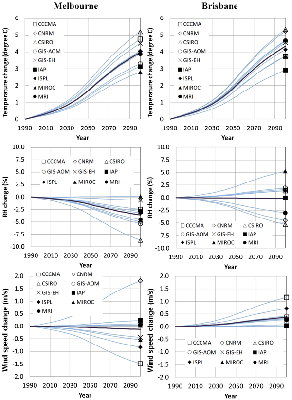
Projected changes of temperature, RH and wind speed for Melbourne and Brisbane under A1FI scenario: in each plot, thin curves are of nine GCMs and thick curve denotes average

Projections of changes in corrosion rates

In the previous section, it was indicated that there are three useful parameters related to atmospheric corrosion that are projected by existing climate change models. These are the temperature, RH and wind speed. In the following, these parameters will be integrated into the atmospheric corrosion model developed by Nguyen et al.16

Taking 1990 as the reference year, the climate change factor due to temperature change, C _temp, can be defined using equation (7) (8) where T ₁₉₉₀ is the absolute yearly average temperature at year 1990, T _projected is the projected absolute yearly average temperature due to climate change in the future and and are corrosion rate parameters at T ₁₉₉₀ and T _projected respectively.

Similarly, by equation (5), the climate change factor for the time of surface wetness due to the change in RH is defined as (9) where RH ₁₉₉₀ is the RH at the reference year 1990. RH _projected is the projected RH due to climate change. t _wet,1990 and t _{wet,projected} are the times of surface wetness at RH ₁₉₉₀ and RH _projected respectively.

The airborne salinity S _air in equations (3) and (4) is stated in terms of deposit on a salt candle29 and needs to be related to the volumetric airborne salinity S _air,vol. Cole and Corrigan41 expressed the relationship by (10) where η is a deposition efficiency factor, and A _s is the area of the salt candle surface that the salinity aerosol impacts on. 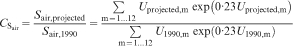Using equations (6) and (10), the climate change factor can be expressed as (11) where is the projected airborne salinity due to climate change and is the airborne salinity at the reference year 1990. U _1990,m is the mean wind speed for month m of the reference year 1990; U _projected,m is the projected mean wind speed for month m of the projected year under climate change. The monthly mean wind speeds were used to capture the effect of seasonal changes of wind speed on the airborne salinity. This is consistent with the airborne salinity model used by Nguyen et al.16 The values of U _projected,m have been computed by applying the values shown in Fig. 3 as modification factors to the values of U _1990,m. It is also to be noted that an implicit assumption in all of this is that the relative change in wind speed will be the same for all directions, i.e. the changes will not be dominant in a specific direction.

Using equations (3), (4), (8), (9) and (11) into equations (3) and (4) leads to C _rate,zinc and C _rate,steel, the projected relative corrosion rates of zinc and steel (12) The terms C _rate,zinc and C _rate,steel indicate increases in the corrosion rate when they are >1·0 and indicate decreases in the corrosion rate when they are smaller than 1·0, in comparison with the rate in 1990. The difference between the factors and 1·0 gives the percentage of the changes in corrosion rates caused by climate change.

Using equations (8), (9), (11) and (12), the three climate change factors C _temp, and and the relative corrosion rates C _rate,zinc and C _{rate, steel} were estimated every 5 years from 1990 to 2100 using the climate change effects projected from each of the nine GCMs under the A1FI emission scenario. Because the climate projection data, i.e. T _projected, RH _projected and U _projected,m in particular, are changing with time (Fig. 3), the climate change factors and the relative corrosion rates also change with time.

The climate change factors C _temp, C _wet and from 1990 to 2100 are shown in Fig. 4. Comparative plots of these three parameters are shown in Fig. 5; these plots show the relative influence of the three climate change factors. Finally, the relative corrosion rates C _rate,zinc and C _rate,steel from 1990 to 2100 are shown in Fig. 6 and given in tabulated form in Table 3.

Figure 4

Climate change factors C _temp, and for Melbourne and Brisbane under A1FI scenario: in each plot, thin curves are of nine GCMs and thick curve denotes average

Figure 5

Comparison of average of three climate change factors C _temp, and for Melbourne and Brisbane under A1FI scenario

Figure 6

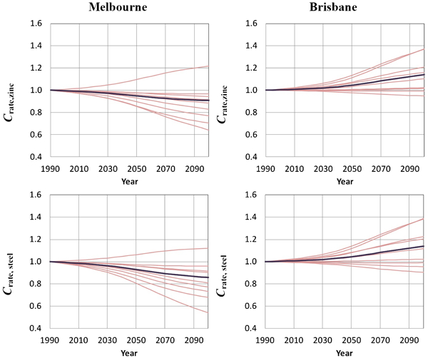
Effects of climate change on relative corrosion rates C _rate,zinc and C _rate,steel for two cities under A1FI scenario: in each plot, thin curves are of nine GCMs and thick curve denotes average

Table 3

Average effects of climate change on relative corrosion rates at certain years for Melbourne and Brisbane under A1FI scenario

City	Relative corrosion rates	Year 2030	Year 2050	Year 2070	Year 2100
Melbourne	C _rate,zinc	(0·927-1·047)	(0·853-1·096)	(0·761-1·154)	(0·642-1·216)
	C _rate,zinc	0·973	0·949	0·926	0·907
	C _{rate, steel}	(0·903-1·032)	(0·806-1·063)	(0·687-1·096)	(0·539-1·121)
	C _{rate, steel}	0·963	0·929	0·893	0·858
Brisbane	C _rate,zinc	(0·989-1·062)	(0·978-1·135)	(0·964-1·235)	(0·948-1·373)
	C _rate,zinc	1·020	1·045	1·083	1·139
	C _{rate, steel}	(0·980-1·065)	(0·959-1·140)	(0·934-1·244)	(0·903-1·388)
	C _{rate, steel}	1·019	1·045	1·082	1·138

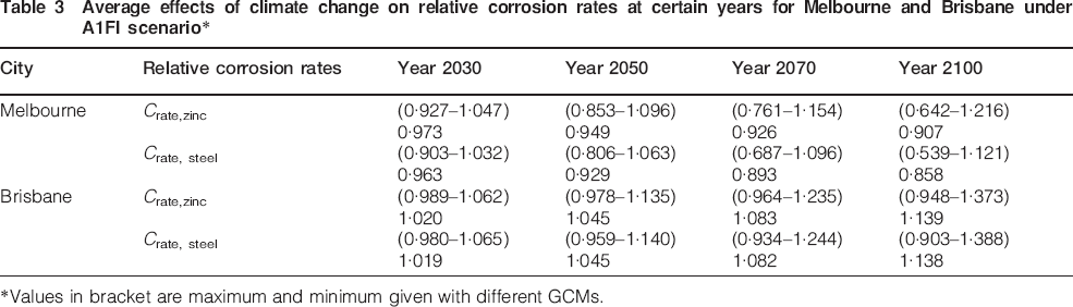
*Values in bracket are maximum and minimum given with different GCMs.

Discussion

Computed changes in corrosion rates

As can be seen in Fig. 5, the most influential parameters affecting changes in corrosion rates were in the case of Melbourne and in the case of Brisbane. As shown by equations (9) and (10), these changes relate to changes in the RH _projected (projected annual RH) and U _projected,m (projected monthly wind speed) respectively. The effect of temperature on the corrosion rate, represented by C _temp, is negligible.

It is of interest to note that for the period 1990-2100, the projected relative corrosion rates decreased in the case of Melbourne and increased for Brisbane. On average, in 2100, the average projected climate change impact in Brisbane is increases by ∼14% in the relative corrosion rates of steel and zinc, while the projected climate change impact on relative corrosion rates in Melbourne is a reduction of ∼14% for steel and 9% for zinc, as shown in Table 3. However, it is to be noted that if the worst GCM projections are used, then the projected relative corrosion rates for the year 2100 increase for both cities, i.e. by ∼20% for Melbourne and 40% for Brisbane.

Rainfall patterns

Unfortunately, the various climate change models do not provide adequate information on the effect of changes in rainfall patterns to make use of the cutoff concept3 mentioned in the section on ‘Effect of changes in rainfall patterns’ to predict changes in salinity factors. This change relates to the effect of rain in washing off accumulated salt.

A lower limit of this effect can be found by comparing corrosion rates for exposed and sheltered environments. From the Australian model,16 the corrosion rate of exposed elements, relative to that of sheltered element, is derived to be ∼0·7; from the field data by King and O'Brien,42 a typical measured ratio would be ∼0·6. These are extreme cases, giving 30 or 40% increase in the corrosion rate when changing from elements that are fully exposed compared to those that are fully sheltered from rain. Hence, it would not be unreasonable to expect that the increase in corrosion due to changes in rainfall patterns would be of the order of 10% for exposed structures. This is comparable with the projected changes due to other climate parameters discussed in the section on ‘Projections of changes in corrosion rates’.

Moreover, as the reduction in corrosion for exposed constructions is related to the washing effects of rainfall, it is unlikely that engineers will make use of this ‘exposure factor’ in the design of significant structures since it would be unreliable to assume that total exposure to rainfall will be maintained indefinitely.

Uncertainties

In any estimate of climate change effects, it is also important to estimate the uncertainties associated with the estimate. Some idea of the errors due to climate change estimates can be obtained by examining the plots shown in Fig. 6. With some allowance for the variability associated with each GCM model, the uncertainty in projection of the relative corrosion rates for 2100 would correspond to a coefficient of variation of ∼30%.

This degree of uncertainty should be placed in the context of the uncertainty of corrosion modelling that currently exists when climate change effects are not considered. In the application of the Australian model to practical design situations, a value of 200% is recommended to be used for the coefficient of variation in estimating corrosion depths.16 This is an uncertainty considerably larger than the 30% estimated to account for in the application of climate change models.

Corrosion of inland constructions

Under climate change, the atmospheric corrosion rate of steel structures located in the inland areas could possibly increase due to increases of airborne salinity levels, as estimated by Cole and Paterson.3 However, the airborne salinity inland is dominated by ocean produced aerosol, which at the coastline is ∼25 times lower than that of the surf produced aerosol for an open surf location.16 Hence, the atmospheric corrosion of steel inland would be considerably less than that near the coastline and would not normally be a major durability concern.

Depth of corrosion

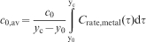
Because the climate change factors are changing with time, and thus the corrosion rate, the corrosion depth up to an in-service duration t is a cumulative corrosion with a changing corrosion rate parameter during the time. However, there is only limited available data that is useful for developing models of corrosion depth under changing environment conditions. In view of the relatively small changes that are projected, it would probably be adequate to use a constant value of corrosion rate parameter c _0,av, an average value to compute the relative corrosion rate over the in-service duration under climate change conditions. The average corrosion rate parameter c _0,av can be computed from (13) where c ₀ is the corrosion rate parameter without climate change effects, τ is a time variable, y ₀ is the year of installation of the structure, y _c is the final year of consideration of the corrosion and C _rate,metal is the relative corrosion rate for zinc or steel as defined in equation (12). The difference between y _c and y ₀ is therefore the in-service duration. This computation approach is similar to that used by Stewart et al. for estimating the carbonation process in reinforced concrete.

Conclusions

A review of corrosion processes has indicated that the relevant science is complex and full of uncertainty. It indicated that care is required in examining the context in which research conclusions have been made. When these facts are added to the difficulties in the use of climate change models, it is realised that there is a considerable complexity and scope for error in making predictions of future corrosion rates.

Within this paper, an attempt has been made to go as far as possible within the available science, to make predictions on future corrosion rates. To do this, existing corrosion and climate change models have been used. Specifically, an existing Australian corrosion model and nine GCMs under the climate change scenario A1FI were used to predict changes in corrosion rates from 1990 to the year 2100. To achieve clarity in presentation, pollution effects were neglected and the applications were limited to the coastal areas of only two Australian cities: Melbourne and Brisbane.

The output parameters of the climate change models that were found to be useful were the projections of RH, wind speed and temperature. Of these, temperature was found to be of very minor significance. Using these parameters, it was found that on average the relative corrosion rates were projected to have a decrease of ∼9% (for zinc) and 14% (for steel) for Melbourne, and an increase of ∼14% for Brisbane in 2100 for both metals.

A major deficiency in the climate projection models was the availability of quantitative data on the rainfall patterns. This would have provided information on the beneficial effects of rain wash on exposed constructions. It is anticipated that this effect will lead to an increase of ∼10% in the predicted corrosion rates for exposed constructions. A refinement of current climate prediction models to assist in these predictions would be useful.

Finally, the matter of uncertainty in climate prediction forecasts was examined. The data appear to indicate the uncertainty in the prediction of corrosion rates, i.e. equivalent to a coefficient of variation ∼30%, whereas the corresponding uncertainty in the Australian model to predict corrosion rates (excluding climate change effects) would be a coefficient of variation of ∼200%. Hence, for engineering design purposes, the uncertainties associated with climate change models are of secondary importance.

Footnotes

Acknowledgements

The authors would like to express their appreciation for the support by CSIRO Climate Adaptation Flagship and the National Climate Change Adaptation Research Facility under the project ‘Pathways to Climate Adapted and Healthy Low Income Housing’. The authors would also like to thank K. Hennessy and J. Clarke of CSIRO Marine and Atmospheric Research and R. Jones of Centre for Strategic Economic Studies at Victoria University for their assistance and advice on climate projections using OzClim.

References

Koch

Payer

Brongers

MPH

Thompson

Virmani

: ‘Corrosion costs and preventive strategies in the United States’ Technical Summary Report, Publication No. FHWA-RD-01-156, Federal Highway Administration. http://www.nace.org/uploadedFiles/Publications/ccsupp.pdf (accessed August 2012).

Ratcliff

: ‘Research shows corrosion costs the local economy’ Curtin News, Curtin University. http://news.curtin.edu.au/news/research-shows-corrosion-costs-the-local-economy/ (accessed August 2012).

Cole

Paterson

: ‘Possible effects of climate change on atmospheric corrosion in Australia’ Corros. Eng. Sci. Technol. 2010 45 (1) 19–26.

Roberge

: ‘Impact of climate change on corrosion risks’ Corros. Eng. Sci. Technol. 2010 45 (1) 27–33.

Graedel

Leygraf

: ‘Scenarios for atmospheric corrosion in the 21st century’ Electrochem. Soc. Interface 2001 24–30.

Bastidas-Arteaga

Chateauneuf

Sanchez-Silva

Bressolette

Schoefs

: ‘Influence of weather and global warming in chloride ingress into concrete: a stochastic approach’ Struct. Saf. 2010 32 238–249.

Stewart

Wang

Nguyen

: ‘Climate change impacts and risks of concrete infrastructure deterioration’ Eng. Struct. 2011 33, 1326-1337.

Wang

Stewart

Nguyen

: ‘Impact of climate change on corrosion and damage to concrete infrastructure in Australia’ Clim. Change 2012 110 (3-4) 941–957.

Benarie

Lipfert

: ‘A general corrosion function in terms of atmospheric pollutant concentrations and rain pH’ Atmos. Environ. 1986 20 (10), 1947-1958.

10.

Feliu

Morcillo

Feliu

: ‘The prediction of atmospheric corrosion from meteorological and pollution parameters. II: long-term forecasts’ Corros. Sci. 1993 34 (3) 415–422.

11.

de la Fuente

Castaño

Morcillo

: ‘Long-term atmospheric corrosion of zinc’ Corros. Sci. 2006 49, 1420-1436.

12.

Melchers

: in ‘Modeling of corrosion of steel specimens in natural waters’, ( Kain

R M

Young

W T

). Vol. 220–33; 1997

Philadelphia, PA

American Society for Testing of Materials.

13.

Melchers

: ‘Advances in mathematical modelling of the atmospheric corrosion of structural steel in ocean environments’ Proc. 3rd Int. ASPRANet Colloq. Glasgow, UK: ASRANet Ltd. July 2006 037–005. http://maritime-conferences.com/asranet2010-conference/asranet2006/PDF/037_005_MelchersASRANet06-full.pdf.

14.

Feliu

Morcillo

Feliu

: ‘The prediction of atmospheric corrosion from meteorological and pollution parameters. I: annual corrosion’ Corros. Sci. 1993 34 (3) 403–414.

15.

de la Fuente

Díaz

Simancas

Chico

Morcillo

: ‘Long-term atmospheric corrosion of mild steel’ Corros. Sci. 2011 53 (2) 604–617.

16.

Nguyen

Leicester

Wang

C.-H

Foliente

: ‘Corrosion effects in the structural design of metal fasteners in timber constructions’, Struct. Infrastruct. Eng. 2011 9 (3) 276–285.

17.

‘Hot-dip galvanized (zinc) coatings on fabricated ferrous articles’

Standards Australia

Sydney, NSW, Australia

2006.

18.

Corrosion Doctor: ‘Factor affecting atmospheric corrosion’. http://www.corrosion-doctors.org/Corrosion-Atmospheric/Factors-atmospheric.htm (accessed August 2012).

19.

CSIRO : ‘Climate change in Australia’ Technical Report 2007, CSIRO Marine and Atmospheric Research, Aspendale, Vic., Australia. http://www.climatechangeinaustralia.gov.au/technical_report.php (accessed August 2012).

20.

Pacheco

AMG

Ferreira

MGS

: ‘An investigation of the dependence of atmospheric corrosion rate on temperature using printed-circuit iron cells’ Corros. Sci. 1994 36 (5) 797–813.

21.

Shaw

WJD

Anderson

: ‘Atmospheric corrosion of carbon steel in the prairie regions’ Proc. Northern Area Western Conf. Calgary, Alta., Canada February 2010 NACE International. http://www.nacecalgary.ca/pdfs/NorthernPapers/Atmospheric%20Corrosion.pdf .

22.

NACE : ‘Temperature influence on corrosion’ NACE Resource Center. http://events.nace.org/library/corrosion/design/temperature-effects.asp (accessed August 2012).

23.

Roberge

: ‘Handbook of corrosion engineering’; 1999

New York

McGraw-Hill.

24.

Almarshad

Syed

: ‘Atmospheric corrosion of galvanized steel and aluminium in marine and marine-industrial environments of Saudi Arabia’ Mater. Corros. 2008 59 (1) 46–51.

25.

Lindstrom

Svensson

J.-E

Johansson

L.-G

: ‘The atmospheric corrosion of zinc in the presence of NaCl – the influence of carbon dioxide and temperature’ J. Electrochem. Soc. 2000 147 (5), 1751-1757.

26.

IPCC: in ‘Emission scenarios – special report of the Intergovernmental Panel on Climate Change’, ( Nakicenovic

Swart

); 2000

Cambridge

Cambridge University Press.

http://www.ipcc.ch/ipccreports/sres/emission/index.php?idp = 42#anc1 (accessed August 2012).

27.

Chung

Sung

Hsien

Shih

: ‘Application of EIS to the initial stages of atmospheric zinc corrosion’ J. Appl. Electrochem. 2000 30 607–615.

28.

IPCC: ‘Climate change 2007 – synthesis report – an assessment of the Intergovernmental Panel on Climate Change, IPCC, Geneva, Switzerland’. http://www.ipcc.ch/pdf/assessment-report/ar4/syr/ar4_syr.pdf (accessed August 2012).

29.

Cole

Ganther

Paterson

King

Furman

Lau

: ‘Holistic model for atmospheric corrosion. Part 2: experimental measurement of deposition of marine salts in a number of long range studies’ Corros. Eng. Sci. Technol. 2003 38 (4) 259–266.

30.

‘Atmospheric corrosivity zones in Australia’

Standards Australia

Sydney, NSW, Australia

2008.

31.

King

Martin

Moresby

: ‘A detailed corrosivity survey of Melbourne’

CSIRO Division of Building Research Report

Highett, Vic., Australia

1982.

32.

King

Ganther

Cole

: ‘Studies at sites progressively inland from the coast to aid development of a geographic information system map of Australian corrosivity’ Proc. Conf. on ‘Corrosion and prevention-99’, Sydney, NSW, Australia, November 1999, Australasian Corrosion Association Inc., Paper 39-041.

33.

King

Carberry

: ‘Atmospheric corrosivity of the Greater Newcastle Region’ Technical Report no. TR92/1

CSIRO Division of Building Construction and Engineering

Highett, Vic., Australia

1992.

34.

Cole

: ‘Mechanism of atmospheric corrosion in tropical environments’ in ‘Marine corrosion in tropical environments’( Dean

S W

, ..), 33–47; 2000

West Conshohocken, PA

American Society for Testing and Materials.

35.

Nguyen

Leicester

Wang

C.-H

: ‘Manual no. 5: atmospheric corrosion of fasteners in timber structures’ 2008 Highett, Vic., CSIRO Sustainable Ecosystems.

36.

McKay

Garland

Livesley

Halliwell

Walker

: ‘The characteristics of the shore-line sea spray aerosol and the landward transfer of radionuclides discharged to coastal sea water’ Atmos. Environ. 1994 28 (20), 3299-3309.

37.

Cole

Chan

Trinidad

Paterson : ‘Holistic model for atmospheric corrosion. Part 4: geographic information system for predicting airborne salinity’ Corros. Eng. Sci. Technol. 2004 39 (1) 89–96.

38.

Cole

King

Trinidad

Chan

Paterson

: ‘An Australia-wide map of corrosivity: a GIS approach’ Proc. Int. Conf. on ‘Durability of building materials and components’, Vol. 2901–911; 1999

Vancouver, BC

NRC Research Press.

39.

Wang

Chen

Ren

: ‘Assessment of climate change impact on residential building heating and cooling energy requirement in Australia’ Build. Environ. 2010 45, 1663-1682.

40.

CSIRO: ‘OzClim – exploring climate change scenario for Australia’ http://www.csiro.au/ozclim/home.do (accessed August 2012).

41.

Cole

Corrigan

: ‘Service life prediction of materials’ in ‘Technology, design and process innovation in the built environment’( Newton

, ..), 72–96; 2009

New York

Taylor & Francis.

42.

King

O'Brien

: ‘The influence of marine environments on metals and fabricated coated metal products, freely exposed and partially sheltered’ in ‘Atmospheric corrosion’, ASTM STP 1239, ( Kirk

W W

Lawson

H H

), 167–192; 1995

Philadelphia, PA

American Society for Testing and Materials.

An assessment of climate change effects on atmospheric corrosion rates of steel structures

Abstract

Keywords

Introduction

Review of factors related to atmospheric corrosion

Overview

Effect of changes in rainfall patterns

Effect of changes in RH

Effect of temperature

Effect of pollution

Effects of CO2 concentration

Method for assessment of climate change effects

Models used for atmospheric corrosion

Model for corrosion due to effects of airborne salt

Model for corrosion due to effect of temperature

Climate change models used

Projections of changes in corrosion rates

Discussion

Computed changes in corrosion rates

Rainfall patterns

Uncertainties

Corrosion of inland constructions

Depth of corrosion

Conclusions

Footnotes

Acknowledgements

References

Effects of CO₂ concentration