
Abstract
This paper describes the process for optimising the annealing cycle on a hot dip galvanising line based on a combination of the techniques of artificial intelligence and genetic algorithms for creating two types of regression models. The first model can predict the furnace operating temperature for each coil and is trained to learn from the experience of the plant operators when the process has been correctly adjusted in ‘manual mode’ and from the control system when it has been properly operated in ‘automatic mode’. Once the scheduling has been optimised, and using the two predictive models, a computer simulation is made of the galvanising process in order to optimise the target settings when there are sudden transitions in the steel strip. This substantially improves the thermal treatment, as these sudden transitions may occur when there are two welded coils differing in size and type of steel, whereby a drastic change in strip specifications leads to irregular thermal treatments that may affect the steel’s coating or properties in that part of the coil.
List of symbols
chemical composition of steel, wt‐%
chemical composition of steel, wt‐%
chemical composition of steel, wt‐%
difference in the input temperature of the strip between time t and t+1, °C
difference in the temperature of zone 1 inside the furnace, between time t and t+1, °C
difference in the temperature of zone 3 inside the furnace, between time t and t+1, °C
difference in the temperature of zone 5 inside the furnace, between time t and t+1, °C
difference in the speed of the strip between time t and t+1, m min−1
strip temperature at the heating zone exit, °C
strip set point temperature at the heating zone exit, °C
strip temperature at the heating zone entrance, °C
zone 1 set point temperature (initial heating zone), °C
zone 3 set point temperature (intermediate heating zone), °C
zone 5 set point temperature (final heating zone), °C
strip thickness at the furnace entrance, mm
strip velocity inside the furnace, m min−1
strip width at the furnace entrance, mm
emissivity
Introduction
Predicting and accurately controlling the evolution of the temperature of the steel strip within the annealing process on a hot dip galvanising line (HDGL) is important to ensure both the appropriate thermal treatment to improve the material’s property and the correct diffusion of the zinc coating that is subsequently applied.1 – 3 However, this is no easy matter because HDGLs process coils in a wide range of sizes and types of steel.
One of the overriding purposes of HDGLs is to ensure that the strip reaches the maximum target temperature in the heating zone according to times specified on the annealing curve defined for this type of steel (Fig. 1). It is also clearly very important for this treatment to be uniform over the entire surface of the strip.
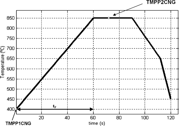
Example of thermal treatment curve in annealing phase
Given the high temperatures involved in the process, it is advisable to preset the target settings for temperature and velocity in the furnace, thereby preparing the system for the incoming coils and ensuring that the thermal treatment is as uniform as possible. Efforts should therefore be made to ensure that the changes in target settings for the temperatures should not be sudden between coils, as furnace inertia means that the real temperatures in the furnace cannot alter very quickly.
Problems arise when certain parts of the coils do not receive uniform treatment, as the steel properties may not be as required and the coating may not be correctly applied.
The main causes tend to be: sudden variations in velocity, the incorrect definition of the target settings for furnace temperature and velocity, coils of different steels or dimensions not considered by the models and sudden transitions between two coils of very different dimensions or types of steel.
The control of most HDGLs is performed in two ways: ‘automatic mode’ and ‘manual mode’.
In the first case, the furnace target settings are handled by a model that seeks to predict the temperature of the final strip according to its dimensions (width and thickness), the velocity of the strip, the steel group, its input temperature and furnace temperatures. These control systems can use analytical models based on differential equations for heat transfer or non‐linear predictive models, such as, for example, neural networks trained with the process data record. At other times, especially when processing coils involving special dimensions or steels, the adjustment of the furnace target settings is performed ‘manually’ by the operator based on past experience and the use of predetermined tables drawn up empirically.
Some studies have been made on the control of the annealing process focusing on the design of mathematical models that explain the complex mechanisms involved in heat transfer due to radiation or convection phenomena that occur inside the furnace, as well as between the latter and the steel strip.1,2,4,5 Other authors, however, such as Bloch et al.,3 conclude that there are complex non‐linear interrelations between all the variables involved in the process that cannot be fully explained by these types of models. The use of non‐linear learning techniques that can learn from the process data record have meant that, in many cases, problems of this nature can be addressed with greater assurances and accuracy.
In recent years, research has been more directed towards the use of neural networks or radial basis function (RBF) networks to improve the control of the process of galvanising.6 – 11 This is due primarily to the fact that these processes and subprocesses are repetitive, highly automated and have a large number of well known variables that define them.
Most of this research focuses on the development of models for predicting the target settings for furnace temperatures according to the strip dimensions and process conditions, although in recent years, consideration has been given to the possibility of modelling the behaviour of the steel strip in order to improve the control of the annealing process on an HDGL.4,12
Martínez‐de‐Pisón et al. 13 considered improving the annealing cycle on an HDGL by designing two models of multilayer perceptron (MLP): the first was used to determine the furnace target settings in steady state, and the second was used to predict strip dynamic behaviour in the event of fluctuations in furnace velocity or temperature. These two models were used to simulate the behaviour of the strip when there were sudden transitions between coils of different sizes, using genetic algorithms to find the best fitting straight line for the target setting signals in order to ensure that the thermal treatment in that zone was as uniform as possible. The problem is that the models were designed for a single group of steels. Accordingly, given the vast range of steels and types of coils processed in an industrial plant, there was a need to create different models for each one of the types of steel existing in the database; this meant investing a great deal of time and effort in generating and validating the various models. Furthermore, it could happen that coils mistakenly listed in the same steel group could have a chemical composition that was substantially different to the rest, whereby they would be incorrectly processed.
This paper presents a combination of data mining (DM) and artificial intelligence (AI) techniques for developing a system, comprising two types of predictive models, capable of optimising the annealing process on a HDGL.
The methodology proposed seeks to redress the bulk of these drawbacks using predictive models that take into account the dimensions and chemical composition of the steel in each one of the coils, with the aim being to develop a scheduling that optimises the process and provides for the definition of certain target settings that ensure that the thermal treatment is as uniform as possible, even when there is a transition between coils of very different dimensions or steels. The process of finding more accurate predictive models involves using GA to fit the parameters of the DM and AI techniques that have recorded the best test results.
Based on these models, it is simple to determine, with a list of the coils to be processed, an appropriate scheduling whereby the furnace temperature varies smoothly when there are changes in the type of coil, and the target setting curves ensure uniform temperature treatment over the entire surface of the coils and, therefore, the right annealing cycle.
Methodology
The methodology used (Fig. 2) involves the following steps:

Methodology proposed to optimise the annealing process on a HDGL
design of an efficient predictive model that allows determining the target settings for the heating temperatures in an annealing furnace on an HDGL in steady state according to the physicochemical parameters of the coils to be processed and the predetermined process conditions (velocity, coil input temperature and target temperature for the strip leaving the furnace). The ultimate aim is to provide a model that can learn, on the one hand, from the operators’ experience when the process has been correctly adjusted in ‘manual mode’ and, on the other hand, from the model for controlling the HDGL when the latter has operated correctly in ‘automatic mode’. Furthermore, the model should be capable of predicting the target settings for the furnace temperatures, not only of the steel coils that have already been processed, but also of new coils with no prior processing record
with a given list of coils to be processed, the optimising of the scheduling to obtain the most appropriate processing velocity, according to the annealing cycle assigned to each coil, as well as target settings for furnace temperatures that are as uniform as possible and which do not change suddenly where there is a transition between coils. The process involves the use of the model obtained in step (i) to calculate the target settings for furnace temperatures that are best suited to each type of coil and its physicochemical specifications (width, thickness and chemical composition of the steel). Finally, the coils are sorted according to the target setting obtained in the end part of the furnace
design of an overall dynamic model that allows predicting the temperature the steel strip will reach when it leaves the heating zone in the furnace on the HDGL, at a moment later, based on current processing conditions, the variation that is expected to exist in them and the physicochemical specifications of the strip at that moment. The ultimate aim is to develop an effective model that can explain strip dynamic behaviour in the event of fluctuations in velocity or temperature in the furnace and for any type of steel or dimensions (width and thickness)
the two predictive models are used for the computer simulation of the galvanising process of the now optimised scheduling of the coils to be processed. This simulation process is used to determine the target settings, in steady state, of the process for each one of the coils. In addition, in the areas of transition between coils, the slopes of the straight lines joining the target settings are optimised to ensure that the annealing temperature of each one of the coils is as uniform as possible and close to the target temperature. This optimisation involves an iterative process with restrictions that fit the slopes on the curves until the difference between the real temperature of the strip and the target temperature is reduced to a minimum
Finally, the optimised curves for the target settings are saved ready to be sent to the system controlling the furnace on the HDGL.
The search for accurate models that generalise the problem well is based on the testing of a series of different techniques arising from DM and AI in order to identify the one providing better predictive models. Genetic algorithms are subsequently used to optimise the parameters for configuring the selected techniques in order to fine tune the degree of accuracy of the final models.
Case study and results
Attributes selection and data preprocessing
Data acquisition was obtained from the computer processing area based on the historic data continuously generated during the galvanising process and consisting of 53 910 records for 1950 coils of 511 different types of steel.
The variables were selected according to their relevance to the furnace heating zone (Table 1). Furnace temperatures, strip velocity and strip temperatures were measured every 100 m along the strip. The strip velocity was measured at the centre of the furnace, and it was reasonable to assume that the strip maintained the same velocity throughout the heating zone.
Relevant variables and their abbreviations
Finally, all the variables were normalised between 0 and 1 to improve the degree of convergence of certain algorithms.
Target regression model
Figure 2 shows the final design of the target models. Three models were designed14 for the target temperature of three zones of the furnace (THC1 = initial zone, THC3 = intermediate zone and THC5 = final zone).
There were 19 input variables in the model (14 of them for the chemical composition of the steel), so principal component analysis (PCA) was used to reduce dimensions and eliminate the high level of dependence between these last variables. From the PCA obtained, the first seven principal components were selected, which cover for 87·44% of the original variance.
Each variable for the chemical composition of the steel was first multiplied by a consensus weight w i, which determined its approximate estimated level of influence into the non‐lineal relations with heat transfer coefficients and thermal emissivity coefficient of the steel ϵ.
Only those cases were selected in which the temperature of the input and output were in a steady state, and the absolute errors of the final temperature of the strip (difference between the target and real temperature of the strip at the exit of the heating zone) were lower than 10°C. In this way, the model learnt to predict the correct temperature settings of the furnace of the strip for the coils with different thickness and widths, both when the settings were controlled manually as well as when the system run automatically. In other words, it learnt both from the experience of the human operator when the process was correctly performed by hand, as well as from the mathematical model when the control was correctly carried out automatically.
A random selection was made from the final database of 434 steels to generate the training database and of another 77 steels for the test database. Special care was taken to ensure that the steels in the training and test database were distributed throughout the entire range of instances. The aim was to have greater guarantees of success when analysing the degree of generalisation of each one of the trained models.
Different algorithms with different configurations were used in order to find the best predictors: M5P algorithm15 (M5P), which implements routines for generating regression trees, MLP16 with least mean square error (LMS) and least mean log squares error (LMLS)17 error criteria, radial basis networks16 (RBFN), linear regression (LINREG), LeastMedSq18 algorithm (LMSQ), which implements a least median squared linear regression, and IBk19 (IBk), which is a version of the k nearest neighbour algorithm. WEKA20 suite and AMORE21 library from R22 software were used to develop the different models.
For the determination of the algorithm or group of algorithms that provided the best prediction, 10 models of the configuration of each type of algorithm were trained with 70% of the data, and the remaining data (30%) were used for validating each model.
To evaluate the models, root mean squared error (RMSE) and mean absolute error (MAE) for different coils other than those used for model construction were used. These errors were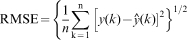

In an attempt to create an overall prediction model capable of determining the temperature settings in the heating area of an HDGL annealing furnace, the models, tested with test database of 77 steels, which proved best able to predict settings for new types of steel coil with dimensions and chemical compositions not previously encountered, were robust MLP networks (LMLS) with three, five or seven neurons in their hidden layer.
Table 2 presents the results of the best predictive techniques obtained for THC1, THC3 and THC5.
Test errors for THC1, THC3 and THC5 from new database with new coils with different dimensions and chemical steel composition
Once the conclusion had been reached that the LMLS algorithm with few neurons in the hidden layer was the one that generated the best predictive models, a search was made with genetic algorithms in order to fine tune the parameters of the selected algorithm. The process focused on the search, within a pre‐established range, for the parameters of the LMLS algorithm that generated the models with the best fit. There were three parameters: the number of neurons in the hidden layer, the global learning rate and the global momentum. The search ranges are shown in Table 3.
Search range set for parameters to be fitted to LMLS model
First of all, 25 LMLS models were trained and validated with different parameters within the ranges shown in Table 3. These models constituted generation 0.
The training and validation process was similar to the one undertaken previously; in other words, 10 models of each configuration were trained with 70% of the training database comprising 434 steels, obtaining the validation errors with the other 30%.
Those of the many individuals in generation 0, which have the lowest RMSEs, were selected and used as the basis for obtaining the next generation (generation 1) by means of crosses and mutations.
The new generation was made up as follows:
20% comprised the best individuals from the previous generation (parents of the new generation)
65% comprised individuals obtained by crossovers from selected parents; the crossover process involves changing various digits in the chromosomes of the variables to be modified, and these chromosomes are made up of the digits for the variables with the decimal points removed, joined together in a single set
the remaining 15% was obtained by mutation through the creation at random of chromosomes within the ranges established; the aim was to find new solutions in areas not previously explored.
This process was repeated over several generations until the RMSE of the best individual was observed to remain the same or not to drop significantly from one generation to the next. Best individual was selected as the final solution.
Finally, test errors with test database were calculated using last generation to compare with previous test results. GENALG library from R software was used to optimise the different models.
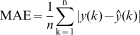
Figure 3 shows the evolution of the RMSE of the best individual for models THC1, THC3 and THC5. After 30 generations, the validation error of the best models fell slightly in models THC1 and THC5, although it improved in model THC3. Table 4 shows the validation and testing models with a new database of coils for the three models before and after optimisation with GA. As can be seen, the final test errors for the best models did not exceed 3% RMSE.
Root mean squared error (RMSE) of best individual in each generation for THC1, THC3, THC5 and strip dynamic model
Final results of best target model for THC1, THC3 and THC5
Optimising scheduling
Once a regression model had been obtained for accurately predicting the target temperatures for the furnace according to the physicochemical specifications of the coils to be processed and to the actual process conditions, the process of optimising the scheduling was addressed.
The reason for optimising the list of coils to be processed was to ensure that the changes in temperature were as smooth as possible so that the temperature in the furnace would quickly adjust to each new type of coil, thereby making the thermal treatment as uniform as possible.
The optimising process involved the following steps:
obtaining the temperatures for the initial target setting (TMPP1CNG) and maximum heating (TMPP2CNG) based on the annealing curves for each one of the coils to be processed. Extraction of the physicochemical specifications of each coil (THICKCOIL, WIDTHCOIL and chemical composition of the steel)
calculation of the target velocity for each coil according to
equalisation of the furnace input temperature for each coil (TMPP1) with the initial temperature of the annealing curve (TMPP1CNG), as it was observed that TMPP1 easily reached TMPP1CNG for each one of the coils that had been processed, and, therefore, there was a minimum error between them
prediction with the target model and using the values of the input variables calculated in steps 1–3 of the target temperatures for zones 1, 3 and 5 (THC1, THC3 and THC5 respectively) in the furnace for each one of the coils on the list
sorting the list of coils according to the volume of steel by square metre according to
sorting the list of coils in step 5 according to THC5.
Figure 4 shows a sample of the first coils in a scheduling comprising 694 coils corresponding to a 15 day process projection.
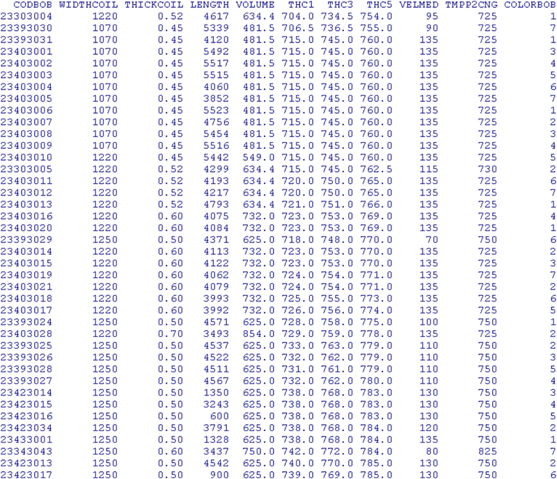
Example of first coils in scheduling of 694 coils to be processed over 15 days
Figure 5 shows the target temperature curves for the furnace before and after the optimisation of the scheduling. In this case, as can be seen in the histograms in Fig. 6, the jumps in temperature were significantly reduced, as they did not exceed 5°C for THC5, with THC1 and THC3 being almost completely below 25°C.
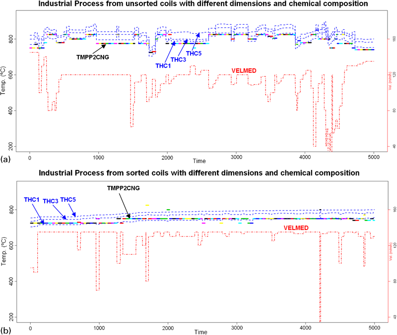
Target setting curves for first 50 000 m of strip
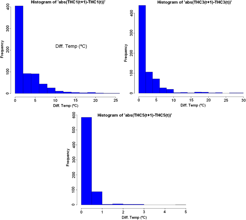
Histogram showing difference between temperature jumps in zones 1, 3 and 5 (THC1, THC3 and THC5) in furnace after sorting list of coils
Model of dynamic behaviour of steel strip
Using the target model, and once the scheduling had been adjusted, it was possible to determine, for the entire list of coils, the target values in steady state for strip velocity and furnace temperatures.
The last step involved designing an accurate model that could predict the temperature that each strip would reach according to the variations in temperatures and velocities in the furnace, its dimensions and the steel’s chemical properties. This model meant that it was possible to simulate the process and fit the slopes of the straight lines joining the target settings in those transition zones between coils with very different physicochemical specifications with a view of ensuring that the thermal treatment was uniform at those times.
The design of the regression model is shown in Fig. 2. The purpose of this model was to predict the temperature of the strip upon leaving the heating zone at time t+1 [TMPP2(t+1)] according to the chemical composition of the steel at that moment, THICKCOIL(t), WIDTHCOIL(t), VELMED(t), TMPP1(t), TMPP2(t), THC1(t), THC3(t), THC5(t), the difference in the input temperature of the strip between time t and t+1 [DIFFTMPP1(t)], the difference in the speed of the strip between time t and t+1 [DIFFVELMED(t)] and the difference in temperatures in each one of the zones in the furnace between time t and t+1 [DIFFTHC1(t), DIFFTHC3(t) and DIFFTHC5(t)).
Given that the model had too many input variables (23), above all due to the high number of elements (14) in the chemical composition of the steel, PCA was used to reduce the high dimensionality and eliminate the high dependence between them.
Accordingly, three PCAs (PCA1, PCA2 and PCA3) were made, grouping the variables corresponding to chemical composition, temperature and temperature differences. From the PCA1 obtained, a selection was made of the first seven main principal components that explained 88% of the original variance, from PC2 the two principal components manage to explain 97% of the existing variance and from PC3 two principal components explained 89% of the total variance. Finally, the model for predicting the temperature of the strip consisted of 15 input variables and one output.
The process of finding the best predictive model was similar to the one for the previous model. A search was made first for the technique that generated the best models. When the models were compared with data from new coils, LMLS‐MLP neural networks with numbers of neurons between 7 and 20 performed far better than k neighbour and M5P based algorithms (Table 5).
Test errors for strip dynamic behaviour model
Genetic algorithms were subsequently used to optimise the parameters of the algorithm chosen to provide the most accurate model possible.
Figure 3 shows the evolution of the RMSE for the best individual in each generation for the strip dynamic model. After 30 generations, the validation RMSE for the best model fell from 2·75% before optimising with GA to 2·25%, and the test error with a new database of coils fell from 3·11% before optimising to a final error of 2·71% after optimising with GA. Figure 7 shows an example of the temperature prediction for the strip with the chosen model.
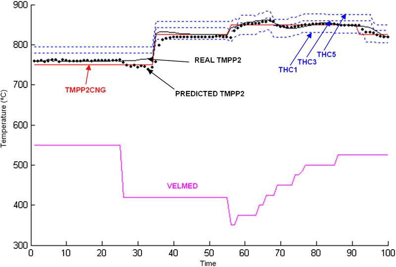
Real temperature of trip (REAL TMPP2) versus temperature predicted by model
Adjusting target setting changes in coil transitions
Using the target model and the strip dynamic behaviour model, it was possible to optimise the slopes on the transition lines for the strip’s velocity and temperature settings in the three zones inside the furnace. The aim was to ensure that annealing for each one of the coils was as uniform as possible on those parts of the strip where there was a sudden transition between coils of different dimensions or types of steel. In other words, the aim was to reduce the mean error between real and target temperature by seeking straight lines that smoothly fitted the transitions of the target curves for the temperature in the three zones in the furnace and for strip velocity.
Optimisation was performed by means of an iterative simulation process with restrictions that could find the width (Fig. 8) of the straight line in order to minimise, in that transition, the error between the real temperature of the strip and the target.
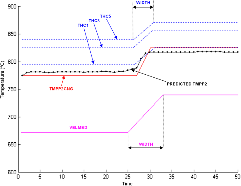
Example of optimising of fitting straight lines in transition of coils with different physicochemical compositions
The process involved the following steps:
use of the target model for generating, based on the list of coils, the curves corresponding to the steady state of the furnace’s target temperatures in zones 1, 3 and 5 (THC1, THC3 and THC5) and the velocity of the strip (VELMED)
definition of the minimum and maximum fitting straight line to be found for the transition lines of the furnace’s target temperatures in zones 1, 3 and 5 (THC1, THC3 and THC5) and the velocity of the strip (VELMED)
search for the moments at which sudden transitions occur between coils with different physicochemical specifications
for each transition found, performance of four nested loops of THC1, THC3, THC5 and VELMED between the minimum and maximum values of the same, thereby obtaining all the possible combinations of widths for the transition straight lines. For each one of the combinations, generation of the transition straight lines and use of the strip dynamic model was used for simulating strip behaviour in that transition. Each simulation provides the error as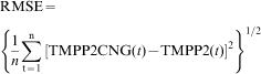
once specification has been made of the optimum widths of the straight lines for all the transitions, generation of the final target setting curves of THC1, THC3, THC5 and VELMED for the entire scheduling of coils is carried out.
Although an intensive search method was used, the simulation was performed quickly as it was noted that making the fit for each transition in R took an average of 5 min in a dual quad‐core Opteron server with Linux SUSE 10·3. Thus, for example, the fit of the transition curves for a 15 day production of 693 coils with 248 transitions required around 21 h to complete, which is a perfectly reasonable amount of time.
For practical purposes, it was not deemed necessary to effect the scheduling for more than 15 days, as it often happens that urgent orders are included for periods of more than 2 weeks that have not been planned for beforehand.
Conclusions
This paper has described a case involving the optimising of the annealing of an HDGL based on its data record. The process involves the creation of two predictive models: one model that learns from the optimum target signals created by the control systems or the operators themselves when the work has been properly carried out and another model that simulates strip dynamic behaviour in the event of variations in temperature and velocity.
These two models can be used to optimise the scheduling of coils and simulate the process in the computer in order to fit the transition straight lines between different coils in order to ensure that the thermal treatment is as uniform as possible.
With a view to obtaining models that can be used with any kind of coil, an intensive search is made involving several DM and AI techniques to find the algorithm that generates the best predictive models. Finally, genetic algorithms are used to optimise the parameters for the best algorithm found. This means that the models provided are highly efficient.
This case may potentially be applied to other types of processes for which a data record is available.
Footnotes
Acknowledgements
The authors thank the ‘Dirección General de Investigación’ of the Spanish Ministry of Education and Science for the financial support of project no. DPI2007‐61090 and the European Union for project no. RFS‐PR‐06035.Finally, the authors also thank the Autonomous Government of La Rioja for its support through the 3° Plan Riojano de I+D+i.