Numerical simulation of fluid flow and solidification in continuous slab casting mould based on inverse heat transfer calculation

Abstract

A mathematical model based on an inverse heat transfer calculation was built to determine the heat flux between the mould and slab based on the measured mould temperatures. With K–ϵ turbulence model, a mathematical model of three-dimensional heat transfer and solidification of molten steel in continuous slab casting mould is developed. Solidification has been taken into consideration, and flow in the mushy zone is modelled according to Darcy’s law as is the case of flow in the porous media. The heat flux prescribed on the boundaries is obtained in the inverse heat conduction calculation; thus, the effect of heat transfer in the mould has been taken into consideration. Results show that the calculated values of mould temperature coincide with the measured ones. Results also reveal that the temperature distribution and shell thickness are affected by the fluid flow and heat transfer of slab which is governed by the heat flux on the mould/slab interface.

Introduction

The phenomena taking place in the continuous casting process are complex, especially in the mould region, where the mushy zone exists and turbulent flow dominates. Modelling of fluid flow and solidification close to reality depends on the accuracy of heat transfer modelling. One of the difficult tasks in fluid flow and solidification simulation is obtaining the heat flux at the mould/slab interface. However, it is difficult to directly measure the heat flux. In such case, a mathematical model of the inverse heat transfer will be a precondition to determine the boundary condition for the fluid flow and solidification simulation.

As early as in 1954, Savage and Prichard1 proposed a formula expressing for heat flux in the mould region based on the measurements. Brimacombe and co-workers2 developed a three- dimensional heat flow model of the mould wall to characterise the heat flux in the mould quantitatively from the measured mould temperature data. Many researchers3 ^– 6 made great efforts in predicting the heat flux at the slab surface. The methods adopted by various researches for the assessment of interface heat transfer were mostly based on the inverse heat conduction problem. Besides, since the 1980s, when Patankar’s classical CFD algorithm, the SIMPLE series methods,7 came into being, study of turbulent flow related phenomena within the caster mould has always been a focus. Seyedein and Hasan8 investigated the flow patterns, heat transfer and solidification process in a continuous casting slab mould using SIMPLE method with K–ϵ model employed. Thomas et al. ⁹ 9,10 also calculated the temperature distribution in the mould, from both the steady state, time averaged velocity field found by standard K–ϵ model and simultaneous flow aspects gained by LES.

This paper presents a numerical simulation on heat transfer between the mould and the slab with a mathematical model of inverse heat conduction problem based on the measured mould temperature. Furthermore, the coupled turbulent flow, heat transfer and solidification of molten steel with practical heat flux boundary conditions are numerically simulated within the mould.

Mould temperature measurements

To provide the mould temperature values for the inverse heat conduction calculation, totally 48 thermocouples were symmetrically buried in the four mould plates, i.e. 18 thermocouples in each of wide faces and six in each of narrow faces. The width, thickness and height of the mould inside dimension are defined in the coordinates of x, y and z respectively. Figure 1 shows the thermocouples x–z location in a wide face and the thermocouples y–z location in a narrow face of the mould. The thermocouples tips in each wide faces are at 15 mm away from the mould inner surface (along the y direction, or vertical to the plane of Fig. 1a ) and those in each narrow faces are at 16 mm away from the mould inner surface (along the x direction, or vertical to the plane of Fig. 1b ).

Figure 1.

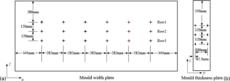
Thermocouples layout in a width plate and b thickness plate at longitudinal sections of mould

Mathematical model

Inverse heat conduction calculation in mould and slab

In order to determine the mould/slab interface heat flux by a measured temperature distribution at the internal points near the mould inter surface, inverse problem method is used in heat transfer calculation of the mould and slab. This method is based on a minimization of error between the calculated and measured temperature at given locations of the thermocouples. Assumptions are made as the following to simplify the inverse heat conduction calculation in the mould and slab:

the continuous casting process is at steady state and the heat conduction along the casting direction is ignored

ii.

the heat transfer caused by the fluid flow in the molten steel of slab is treated with an effective heat conductivity

iii.

the temperature of cooling water in the mould jacket linearly varies from the bottom to the top.

The heat conduction at steady sate in the steel and the mould is governed by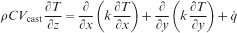 (1) For the molten steel (2) and f _s is linearly defined by (3) where ρ is the density of slab or mould, C is specific heat, V _cast is casting speed, T is the temperature, k is the heat conductivity, is thermal source, H is the enthalpy and f _s is the solid fraction of steel. T _l and T _s represent the liquidus and solidus of steel respectively.

The boundary and interface conditions are as follows:

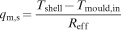
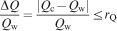
Mould/slab interface heat flux (4) Mould/cooling water boundary heat flux (5) (6) where q is heat flux, and the subscripts m, s and w mean the mould, slab and water respectively. R _eff is the effective thermal resistance between the mould and the slab, T _shell is the surface temperature of the slab, T _w is the temperature of cooling water, h _w is the convective heat transfer coefficient of cooling water, and T _mould,out and T _mould,in are the temperatures at the mould hot wall (mould inner surface) and mould cold wall respectively. Because of the forced convection in the mould water jacket, Dittus–Boelter equation¹¹ 11,12 is introduced to solve h _w. In equation (6), D is the effective hydraulic diameter of the cooling water channel in mould jacket. Variables of k, ρ and C with the subscript of w in equation (6) mean the specific properties of water as similar to those in equation (1). u _w is the velocity of cooling water estimated according to the water flowrate, and μ _w is the molecular viscosity of cooling water.

The convergent conditions for the inverse heat conduction calculation are expressed as equations (7) and (8). Generally, the converged result can be obtained after about 40 iterations. (7) (8) (9) where is temperature measured in the mould at the given location (Fig. 1), is temperature calculated, N _m is number of the thermocouples in the width plate or the thickness plate, i.e. 18 or 6, Q _c is the heat amount released at the mould inner surface, and Q _i is equivalent to the heat flux at the mould/slab interface q _m,s, while Q _w is the heat amount absorbed by the cooling water in the mould. ΔT _w is the temperature increase of outlet water from the mould compared to that of inlet water. r _T and r _Q are the maximal errors permitted in the calculation.

Coupled fluid flow and heat transfer in mould

The coupled fluid flow and heat transfer simulation in the mould is carried out with the heat transfer boundary condition at the mould/slab interface (i.e. q _m,s) obtained by the foregoing inverse problem calculation.

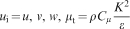
Fluid flow equations

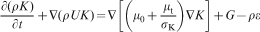
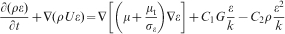
Time averaged governing equations are adopted in this study. Equations governing incompressible viscous flow of Newtonian fluid, i.e. molten steel are Navier–Stokes equations which describe fluid motion, and continuity equation which ensures the continuity condition. K–ϵ turbulence model for high Reynolds number fluid flow is used to calculate the Reynolds stresses in this model.

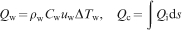
Continuity equation (10) Navier–Stokes equation (11) where (12) K–ϵ turbulence equations: (13) where U(u, v and w) is velocity and S _i is the source term of momentum equilibrium which involves gravity. K is the turbulent kinetic energy, ϵ is the turbulent dissipation, G is the shear production, μ ₀ is the molecular viscosity of molten steel and μ _t is the turbulent viscosity. C ₁, C ₂, σ _K and σϵ are empirical constants.

Energy equations

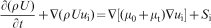
Taking into account the coupled fluid flow and heat transfer of steel in the mould, energy equations for heat transport and temperature distribution are to be solved which can be expressed as the flowing form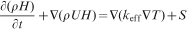 (14) where k _eff represents the effective conductivity. The relationship of enthalpy H and temperature T is shown in equation (15) (15) where h is the static enthalpy and C _p is specific heat of steel.

In calculating aspect, with turbulent transport property considered, k _eff consists of two components (16) where k ₀ is the heat conductivity, treated as constant; k _t is the term responsible for turbulent conductivity (17) When solidification process is coupled with turbulent flow, the existence of two-phase region (mushy zone) greatly influences the flow behaviour in it. A bonding method is used to treat solidified steel as solid wall while the flow in the mushy zone is treated adopting Darcy’s law. Momentum equation is formulated as flowing (18) where S _d represents an additional momentum sink term and can be solved by (19) In current work, the model of Blake–Kozeny13 is utilised to formulate the permeability Γ (20) U is current velocity in mushy zone and K ₀ in equation (20) takes the magnitude of 10⁶. The constant b, introduced to avoid the division by zero, is set at 1×10⁻⁵.

The equations of fluid flow and energy are discretised on a staggered grid of the slab and then solved based on the SIMPLER algorithm14 with the software Visual Cast developed to analyse the continuous casting process.

Calculation conditions

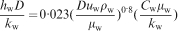
A continuous slab casting is taken into consideration with practical mould temperature measurement and actual submerged entry nozzle (SEN) configuration. Table 1 shows the geometry and process parameters of continuous slab casting investigated in this study. The thermophysical properties of materials for calculation are listed in Table 2. The heat flux in the second cooling region (from 0·9 to 3·0 m under the meniscus) is calculated according to the heat transfer coefficient correlation with cooling water flux in the secondary cooling region.

Table 1.

Geometry and process parameters

Item	Value
Width of slab/m	2·1
Thickness of slab/m	0·25
Height of mould/m	0·9
Height of computation domain/m	3
Casting speed V _cast/m min⁻¹	1
SEN immerge depth/m	0·25
Cooling water flowrate (broad face)/L min⁻¹	4000
Cooling water flowrate (narrow face)/L min⁻¹	600
Temperature difference of cooling water ΔT _w/K	7·6

Table 2.

Thermophysical properties of materials

Item	Value	Item	Value
Density of molten steel ρ _l/kg m⁻³	7·2×10³	Liquidus of steel T _l/K	1786
Specific heat of steel C _p/J kg⁻¹ K⁻¹	842	Solidus of steel T _s/K	1719
Latent heat of steel ΔH/J kg⁻¹	2·75×10⁵	Molecular viscosity of steel μ ₀/kg m⁻¹ s⁻¹	5·6×10⁻³
Thermal conductivity of steel k ₀/W m⁻¹ K⁻¹	34	Molecular viscosity of water μ _w/kg m⁻¹ s⁻¹	7·92×10⁻⁴
Density of mould ρ/kg m⁻³	8·96×10³	Density of water ρ _w/kg m⁻³	998
Thermal conductivity of mould k/W m⁻¹ K⁻¹	366	Specific heat of water C _w/J kg⁻¹ K⁻¹	4·182×10³
Specific heat of mould C/J kg⁻¹ K⁻¹	410	Thermal conductivity of water k _w/W m⁻¹ K⁻¹	0·614

Results and discussion

Figure 2 shows the comparison of the temperature measured and calculated near the inner arc and the outer arc of the mould with the thermocouples x–z position shown in Fig. 1a . Figures 3 illustrates the temperature contours in the transverse x–y section at 280 mm below the top edge in the inner arc and the outer arc of the mould respectively (i.e. at the height of Row 1 in Fig. 2). In Fig. 3, the white dots denote the Row 1 thermocouples location (6×2) and the white area near the mould outer width edge is the water cooling channel. As shown in Fig. 2, the calculated values of mould temperature from inverse problem model coincide with the measured ones. It is found that the temperature at the location of Row 1 thermocouples in both ^{Figure 2} Figs. 2 and 3 fluctuates along the mould width, and this fluctuation is consistent with the uneven cooling strength which is dependent on the arrangement of the water cooling channel as shown in Fig. 3. The temperature fluctuation along the width as shown in Fig. 3 is sensitive when the position is near to the water cooling channel, and the consistency of the temperature fluctuation in Rows 1–3 in Fig. 2 indicates the effect of water cooling channel position.

Figure 2.

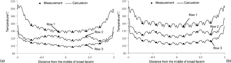
Profiles of calculated and measured temperatures along width direction near a inner arc and b outer arc of mould

Figure 3.

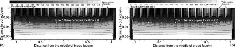
Temperature distribution in transverse section at 280 mm below top edge in a inner arc mould plate and b outer arc mould plate

Figure 4 shows the temperature contours in the inner arc surface and the outer arc surface of the mould respectively. In most of part of the mould wide surface, temperature decreases gradually with increasing distance from the meniscus and with a smaller variation at the mould exit. However, temperature varies rapidly in the vicinity of the mould height edge and near the meniscus.

Figure 4.

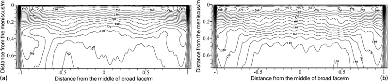
Temperature contours in a inner arc surface and b outer arc surface of mould

Figure 5 indicates the heat flux in the inner arc surface and the outer arc surface of the mould respectively. The non-uniform distribution of heat flux can be found in the width direction. The contour of heat flux is denser near the meniscus and the mould height edge, and heat flux varies smoothly along the casting direction below the middle part of mould. Comparing ^{Figure 4} Figs. 4 and 5, it can be found that an inherent relation exists between the mould surface temperature and the mould/slab interface heat flux which is dependent on the heat transfer conditions, i.e. the structure and dimension of the mould plate and water cooling channel. For example, the heat flux contours will be denser where the temperature contours are denser, and an abrupt variation of heat flux and surface temperature generally locates the meniscus and the mould height edge.

Figure 5.

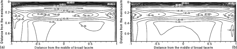
Heat flux in a inner arc surface and b outer arc surface of mould

Figure 6 shows the variations of heat flux along the width direction in the inner arc surface at different locations under the mould top edge of 280, 400 and 520 mm, i.e. the same heights of the first row, the second row and the third row of thermocouples array respectively. Comparing with the three curves, it can be found that the value of heat flux at the height of ‘Row 2’ is higher than those of ‘Row 1’ and ‘Row 3’. Besides, the value of heat flux near the mould height edge is smaller than that in the middle of the mould.

Figure 6.

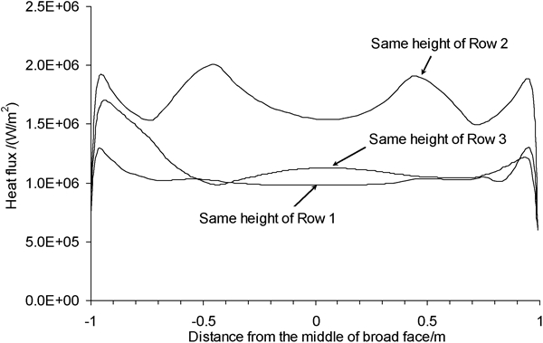
Heat flux along width direction at different heights in inner arc surface

Figure 7 shows the variations of heat flux along the centrelines of the broad and narrow faces. It illustrates that, within 100 mm below the mould top edge, the heat flux is low in the inner arc surface, almost less than 500 kW m⁻², which is followed by a rapidly increasing heat flux until reaches the peak value of almost 3600 kW m⁻² in the region 100–200 mm below the mould top edge, and then decreases quickly but with a smooth variation near the mould outlet. There is the similar changing of heat flux in the other three centrelines. In the middle and lower parts of the mould, heat flux tends to be stable and has little change along the casting direction. As to the non-uniform heat flux at the mould internal surface in ^{Figure 5
Figure 6} Figs. 5–7, it can also be explained by the solidification features and operation process in the continuous casting. During the solidification, the steel contracts and air gap forms beneath a certain distance to the meniscus especially near the mould corner or the mould height edge; therefore, the heat flux becomes smaller. Besides, the heat flux between the mould and the slab may be asymmetry because of unstable operation process such as the uneven water rate in the water cooling channels of the mould.

Figure 7.

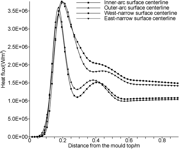
Variations of heat flux at centrelines of broad and narrow faces

^{Figure 8} Figures 8 and 9 illustrate the coupled simulation results of fluid flow and temperature distribution in the slab mould with boundary condition of the mould/slab interface heat flux as shown in Fig. 5. Figure 8 shows the fluid flow in the mid-thickness longitudinal section of the slab. The jets from SEN impinge on the narrow faces and split the whole flow domain into four recirculation zones, two in the upper part and the other two in the downward region. The major vortices that form the lower recirculation zones are located approximately with a distance of 0·8 m below the meniscus. The temperature contour lines in the mid-thickness longitudinal section of the slab are shown in Fig. 9. By comparing the temperature and velocity distribution, it can be found that temperature is affected by the fluid flow in the mould and temperature in both upper and lower recirculation zones, especially in the region close enough to the vortex core, distributes in the way as if it is governed by a Poisson-like transport equation with a predominantly diffusive and isotropic feature. However, in regions far from the centre of recirculation areas, such as near mould wall regions or regions close to SEN ports where convection and turbulent jets dominate, the temperature distribution behaves in an anisotropic way; that is to say, energy dissipates in the flow direction along streamline, as if it is governed by Eular’s transport equation.

Figure 8.

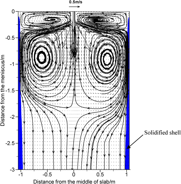
Fluid flow in mid-thickness longitudinal section of slab

Figure 9.

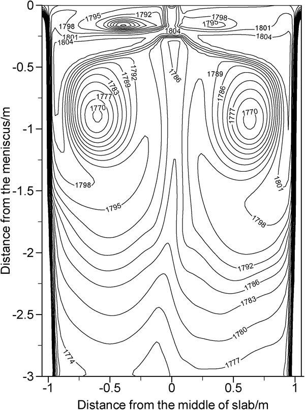
Temperature distribution in mid-thickness longitudinal section of slab

Figure 10 indicates the growth of solidified shell with temperature distribution in the slab cross-section at different height to the meniscus. The dark region in the figure represents the solidified shell. It is clearly seen that the thickness of the shell grows with increasing distance from the monitored cross-section to the meniscus. Simulation results show that the temperature distribution and solidified shell thickness are affected by the fluid flow and heat transfer of slab which is governed by the heat flux on the mould/slab interface (Fig. 5).

Figure 10.

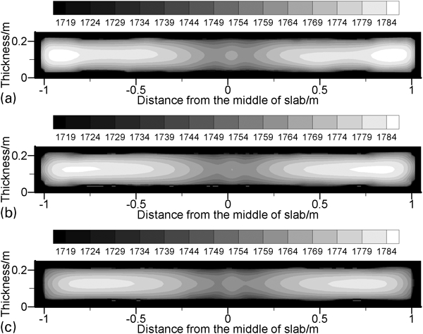
Solidified shell along mould cross-sections of a 1·2 m, b 1·4 m and c 1·6 m from meniscus

Conclusions

In this paper, fluid flow and solidification in the mould were studied based on the real mould/slab interface heat flux obtained by the inverse heat transfer method and the related software named Visual Cast was developed. From the simulation results and discussion above, the following conclusions can be drawn:

The present inverse problem model indicates that the heat flux in the mould/slab interface is non-uniform. Heat flux is smaller near the mould height edge than that in the middle of the mould and the maximum heat flux exists beneath the meniscus. Like the contour of temperature, the contour of heat flux is denser near the meniscus and near the mould height edge. The non-uniform heat flux in the mould/slab interface is consistent with the uneven cooling strength of the mould which is dependent on solidification features of steel, operation process and copper plate geometry, such as the arrangement of the water cooling channel.

Temperature in the slab conforms to such a rule that the temperature gradient changes along the streamline near the jets, or towards the normal direction of streamline in other situations. Regions near vortex’s core are usually low temperature areas.

Results also reveal that the temperature and thickness of solidified shell are affected by the fluid flow and heat transfer of slab which is governed by the heat flux on the mould/slab interface.

Footnotes

Acknowledgements

The authors would like to acknowledge CISDI Engineering Co., Ltd (Chongqing, China) for collaboration. Thanks should also be given to Dr C. L. Zhang and Mr R. Liu at Tsinghua University for their valuable contribution to this research.

References

Savage

Prichard

: ISIJ Int., 1954, 178, (3), 269–277.

Mahapatra

Brimacombe

Samarasekera

Walker

Patersai

Yang

: Metall. Trans. B, 1991, 22B, (6), 861–874.

Saraswat

Maijer

Lee

Mills

: ISIJ Int., 2007, 47, (1), 95–104.

Thomas

: Metall. Mater. Trans. B, 2004, 35B, (6), 1151–1172.

Wang

Samarasekera

: J. Baotou Univ. Iron Steel Technol. (China), 2000, 19, (1), 8–33.

Wang

T.-M

Cai

: China Foundry, 2010, 1, (7), 61–67.

Patankar

: ‘Numerical heat transfer and fluid flow’; 1980, New York, McGraw-Hill.

Seyedein

Hasan

: Can. Metall. Q., 1998, 37, (3–4), 213–228.

Thomas

Zhang

: ISIJ Int., 2001, 41, (10), 1181–1193.

10.

Huang

Thomas

: Can. Metall. Q., 1998, 37, (3–4), 197–212.

11.

Acadams

: ‘Heat transmission’; 1954, New York, McGraw-Hill.

12.

Han

Lee

Yeo

Won

Kim

Yoon

: ISIJ Int., 1999, 39, (5), 445–454.

13.

Poirier

: Metall. Trans. B, 1987, 18B, (3), 245–255.

14.

van Doormaal

Raithby

: Numer. Heat Trans., 1984, 7, 147–163.