Modelling of inertia welding of IN718 superalloy

Abstract

A simple model for the inertia welding of a nickel based superalloy is proposed. The heat flow occurring in the vicinity of the joint is considered, assuming it to be one-dimensional, and this is coupled to a treatment of the stress state expected there using Hill's general method, so that the upset can be estimated. A state variable constitutive model is included, for the IN718 alloy. It is demonstrated that many of the important characteristics of the process are predicted correctly. It is shown that the shear stress developed at the last stage of the process must be accounted if the upset is to be correctly predicted. The results are compared with those from a 2½D finite element model of the process, and the differences rationalised.

Keywords

Inertia welding Analytical model FEM Nickel based superalloys

Introduction

Nickel based superalloys are used widely for hot section components in modern gas engines, e.g. for jet propulsion and electricity generation. Excellent high temperature properties are displayed, particularly in creep, fatigue and oxidation, so that these are then the materials of choice for the turbine and sections of the combustor, where the fuel is burned.1 The fuel economy, propulsive efficiency and rate of carbon emissions of these engines depends critically upon the temperature which can be withstood by these pieces of turbomachinery;2 this situation provides the economic and technological drive for the further improvements in component design which are being sought. New grades of superalloys and processes by which to fabricate components from them are then required.3

Many of the components fabricated from the superalloys have traditionally required some form of joining operation, since net shape manufacturing is not always feasible. For example, electron beam welding is used widely for the joining of sections of the compressor, which consists of a number of discs and rings welded together to form a drum, onto which the compressor blades are arranged. Similarly, the combustor requires the use of fusion welding methods (e.g. the tungsten inert gas process) for the joining of parts made by sheet forming techniques. However, the latest grades of high strength superalloys are not readily amenable to these traditional joining methods. Instead, friction welding techniques are being developed in which a joint is believed to be produced without incurring the gross melting of the material, so that cracking and severe distortion during solidification is avoided. Inertia welding is one such technique. In this paper, modelling of the inertia welding process is considered, with attention being paid to the alloy IN718.

Background

Inertia welding, sometimes known as inertia friction welding or stored energy friction welding,4 has been used widely since it emerged in industry over forty years ago. It can be considered to be a special form of forge welding.5 The workpiece to be joined is first attached to a flywheel and accelerated to a high angular velocity; welding begins when a stationary part is pushed against it after the driving power is shut off, so that the speed of the rotating part drops rapidly eventually reaching zero. Heat is generated by friction, causing a solid state bond to be formed. It follows that inertia welding is carried out under a constant pressure but at changing rotation speeds.6 A schematic illustration of inertia welding is shown in Fig. 1.

Figure 1

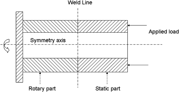
Schematic illustration of inertia welding process

Inertia friction welding can be divided into three stages.7 The first is the heating stage, which is dominated by the dry friction generated under the applied load. Here, the temperature of the mating surfaces rises rapidly in a very short period of time. When the temperature of the surfaces reaches a value close to the melting temperature, the torque drops to a lower, steadier level. This corresponds to a second, so called steady state, stage being reached. It is here that the flash forms, with the torque reaching a maximum at the end of this stage. The third stage is the cooling stage which begins after the flywheel stops. The different stages of the inertia welding process are illustrated in Fig. 2.

Figure 2

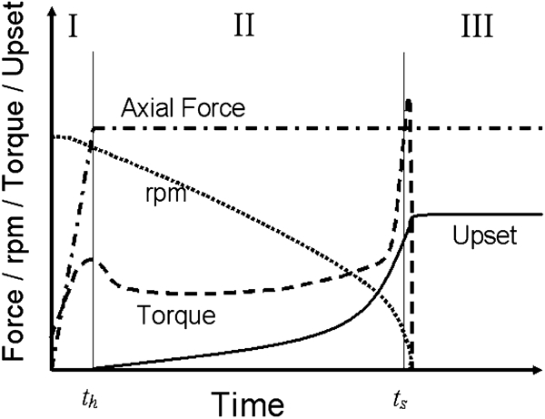
Different stages of inertia welding process.

In practice, many aspects of the inertia welding process are difficult to detect experimentally; this is particularly true of the thermal cycles close to the weld and the associated constitutive behaviour of the material as it softens and deforms plastically. This situation means that analysis of the phenomena occurring by numerical modelling has considerable value. Rykalin et al. were some of the first to consider this problem; they developed a one-dimensional model of friction welding and in particular a closed form solution for the temperature field.8 The assumptions used were semi-infinite solid, an initial temperature and constant thermal material properties; the expression derived is an exact analytical solution for the temperature distribution provided that there is no steady state stage. However, usually this is not the case, and unfortunately this limits the usefulness of this analysis. Healy et al.9 presented an interesting model with a temperature dependent Bingham plastic constitutive equation to describe the behaviour of the plasticised layer. The model gave a reasonable prediction of the change of the torque during the process. However, the axial shortening rates under various rotation speeds and compression loads are needed in this model, which limits its applicability. Francis and Craine modelled the softened material in continuous drive friction welding as a Newtonian fluid of large (but constant) viscosity, but no experimental validation was provided.10 Midling and Grong developed a multistage thermal model for friction welding, in which the related process of continuous drive friction welding was divided into three stages; a closed form solution for each of these three stages was given.7 Although the formulae for the last two are not the exact solutions of heat conduction equation, they can still be used in practice as approximations. Dave et al. presented a model to predict the transient thermal response in the inertia welding of dissimilar tubes based on machine generated process data, including the variation of rotation speed with time and the rate of material burnoff.11 Thermal analysis in friction welding using the finite difference method (FDM) is also possible. In 1962, Cheng made a pioneering attempt with this method.12 Wang and Nagappan made a thermal analysis for the inertia welding of a steel bar; their results confirmed that the peak temperature is reached very quickly as compared to conventional friction welding and that the welding time had a strong influence on the temperature distribution experienced in the vicinity of the weld.13 Most recently, Maalekian et al. proposed an inverse heat transfer model using the finite difference method, and good agreement between predicted temperatures and measured data was reported.14

Recently, use of the finite element method (FEM) has become more commonplace, and this offers the advantage that a mechanical analysis can be coupled to the thermal one. One of the first to use the FEM approach was Sluzalec, who built a thermomechanical FEM model to simulate the welding of mild steels.15 Moal and Massoni studied the inertia friction welding with a FEM model, employing a viscoplastic Norton–Hoff law to describe the material behaviour.16 Fu et al. simulated the inertia welding process using the commercial code DEFORM, with an incremental elastoplastic constitutive relationship incorporated into it.17 D'Alvise also performed a coupled thermal/mechanical analysis to predict the temperature, strain and residual stress field for inertia welds, using the FEM code FORGE2. The model was validated in terms of macroscopic parameters including welding time, total loss of length and flash profile.18 Wang et al. made a simulation of the inertia welding of the high strength superalloy RR1000 using DEFORM.19 In this article, a two-dimensional (2D) model was built with stress, strain and temperature fields being predicted for different boundary conditions. The thermal history was verified by a study of the microstructure in the weld region. The residual stresses were also presented with effects of creep relaxation included. However, the heat flux data was applied directly at the weldline based on energy conservation, derived from experimental data. The mechanical effect of friction, or in other words the friction induced shear stress, was not considered in the model, so the results got from simulation may be quite different from real situations. More recently, Zhang et al.20 made a three-dimensional (3D) simulation of continuous drive friction welding of cylindrical forms using DEFORM. However, no significant advantage of performing 3D rather than 2D calculations was demonstrated. Finally, Bennett and co-workers have made simulations of the inertia welding of dissimilar joints: IN718 to stainless steel AerMet100, with DEFORM.21 In their model, the effect of the phase transformations occurring in the steel on the residual stress fields was emphasised.

In reviewing the literature which has been published already on the inertia welding process, it seemed to the authors that the relative advantages/disadvantages of a simple analytical approach and one based upon the finite element method need clarification. In particular, the extent to which the stress state developed can be approximated without appreciable loss of accuracy needs to be studied. Moreover, it is known that the total upset generated, which is in practice one of the most important parameters which needs to be predicted, is strongly dependent upon the details of the constitutive model used for the description of the stress/strain behaviour. The work reported here was carried out with these factors in mind.

Analytical model for inertia welding process

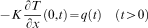
It is necessary to identify the key process variables (KPVs) which can be measured; these can be regarded as inputs to the process model. In the inertia welding process, the axial load P, the initial angular rotating speed ω and the moment of inertia of the flywheel/rotating part I may be regarded as the KPVs. Typically, the variation of ω with time t during the process is recorded during welding; this allows the friction induced torque T to be determined by first estimating the instantaneous value of the angular deceleration a(t) according to (1) and multiplying by the moment of inertia, denoted I, such that (2) Note that the instantaneous value of the angular deceleration can be estimated by an appropriate finite difference expression, provided that the functional form of ω(t) is known. Then, the friction induced shear stress can be estimated by balancing it against the torque, according to (3) where r_n and A refer to the average value of the outer/inner radii and the mating area of the weld being formed respectively. Assuming the axial load P to be constant during the process, the nominal friction coefficient μ in the welding interface can be determined from the ratio of τ, the shear stress developed and the axial normal stress P/A.

It is helpful to insert approximate values into the expressions, in order to fix ideas. It is usual for an axial stress of several hundred MPa to be applied, with an initial angular speed of a few hundred revolutions/min, and the initial total energy of the flywheel to be several million joules. Taking these values to be 250 MPa, 135 rev min⁻¹ and 3×10⁶ J respectively, with an average friction stress of 15 MPa acting on a mating area of order 10000 mm², the time of welding can be estimated to be around 30 s. This estimate is consistent with what is usually observed in practice. Moreover, to a first approximation, the angular speed ω is expected to decrease linearly with time, consistent with constant energy dissipation at the mating surfaces. In practice, the angular speed is found not to decrease linearly with time; instead it decreases rather more slowly initially, with a rather sharp decrease as the weld is finally created (see the curve 2 in Fig. 3). The corresponding shear stress curves are illustrated in Fig. 4; estimates of the way in which the interfacial friction coefficient varies with time μ would follow, as before. Note the sharp increase in the shear stress at the very end of the process, which arises due to the significant rate of change of ω with time at that point. These considerations emphasise the importance of an accurate measurement of ω(t) throughout the process.

Figure 3

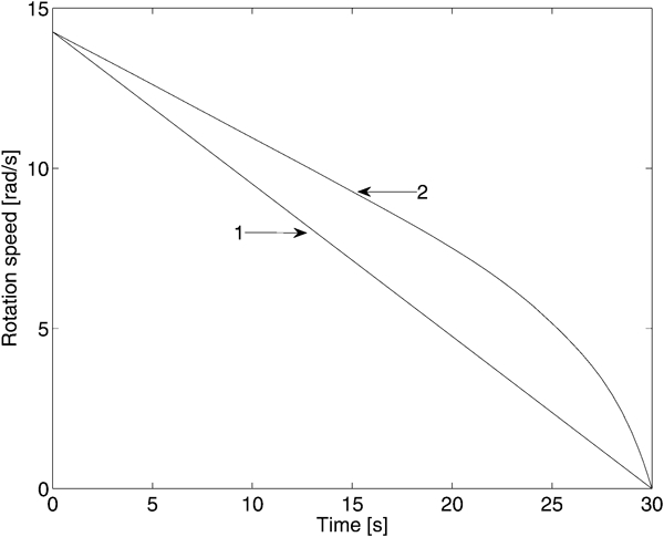
Typical variation of angular speed with time during inertia welding process

Figure 4

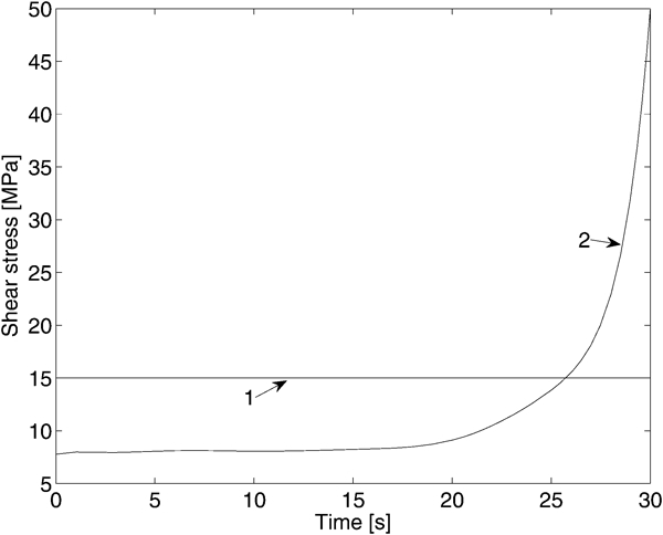
Variation of shear stress with time, corresponding to curves given in Fig. 3

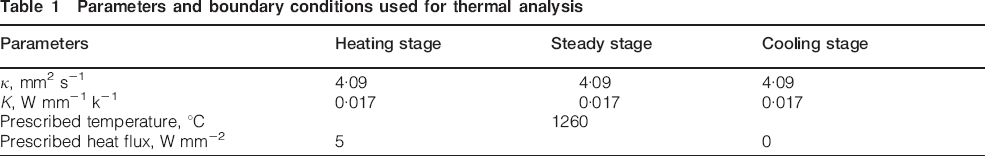
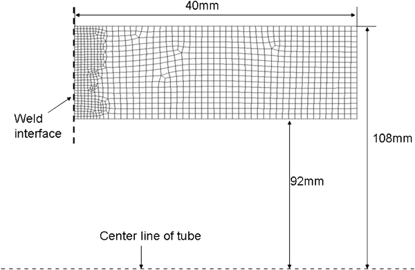
In practice, the geometry of the part to be welded is of considerable importance. Provided that there is radial symmetry, complicated shapes can be joined, but one common arrangement is that of a circular tube, and this will be assumed in the present paper. It will be assumed that two tubes of identical geometry are to be welded, of identical material, taken to be the superalloy Inconel 718. To simulate the welding process of this part and to simplify the thermal analysis, the effects of radiation and convection along the outer and inner surface of the tube will not be taken into consideration. This is expected to be approximately true if the welding process is finished in a short time. The length of the part is taken to extend to infinity where it is clamped rigidly at one end. Thus, a semi-infinite one-dimensional heat conduction model was used, with the weldline located at the origin x = 0, at which a boundary condition of fixed temperature or flux was prescribed, as illustrated in Fig. 5. Only one-half of the weld was modelled. Temperature averaged material properties are adopted in the calculation, and these are summarised in Table 1.

Figure 5

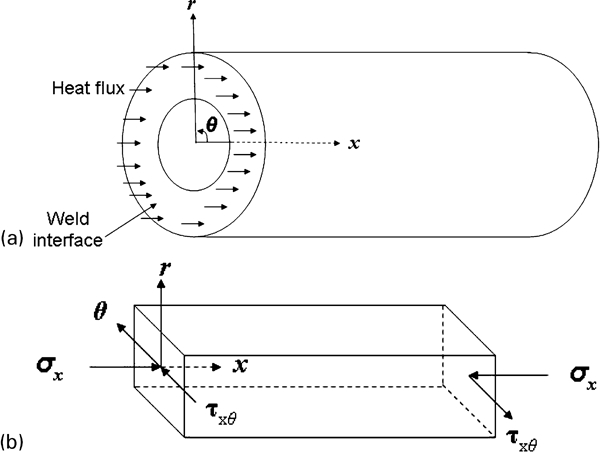
Thermomechanical model used in calculation: a round tube with thermal boundary conditions indicated; b element within it

Table 1

Parameters and boundary conditions used for thermal analysis

Parameters	Heating stage	Steady stage	Cooling stage
κ, mm² s⁻¹	4·09	4·09	4·09
K, W mm⁻¹ k⁻¹	0·017	0·017	0·017
Prescribed temperature, °C		1260
Prescribed heat flux, W mm⁻²	5		0

Thermal analysis: Modelling of heat transfer

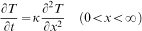
The one-dimensional heat equation to be solved is as follows22 (4) where T, x and t are temperature, distance and time respectively. The term κ = K/ρc is the thermal diffusivity, where K, ρ and c are thermal conductivity, density and the heat capacity of the material respectively. The initial condition is taken as (5) where f(x) is the known function representing the initial condition, i.e. the prescription of the temperature at every point in the body at the initial moment (t = 0). The boundary conditions used for calculation during the heating process are taken as follows (6) and (7) where g(t), the boundary temperature distribution, is an assumed (known) function of time.

Given what is known about the inertia welding process and consistent with the work of others,7 the temperature calculation is carried out in three distinct steps. During the first (heating) stage, the temperature at the weldline rises rapidly; to simplify the calculation, a constant heat flux q(t) is used in this period. In the second stage, the surface temperature at the weldline (x = 0) is assumed to be constant, which is a reasonable approximation due to the dynamic heat balance between heat generation and heat conduction at the weldline. Finally, during the cooling stage the heat flux at the surface is set to zero, consistent with a lack of heat generation and the plane of symmetry along the weldline.

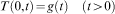
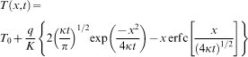
The initial temperature for the parts to be welded is assumed a constant T₀. In the heating stage, T₀ is assumed to be 0°C, i.e. f(x) = 0. This makes the calculation simpler and produces results which are only marginally different from those with a room temperature value of 20°C. The initial temperature for the second stage is taken to be that at the end of the heating stage. 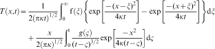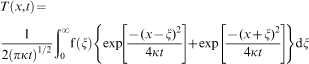The formula for the heating stage is 22 22,23 (8) where q is the heat flux, K is the thermal conductivity, t and x refer to time and the axial coordinate respectively, κ is the thermal diffusivity and erfc(x) is the complementary error function.

For the second stage, one takes22 (9) where f(ξ) refers to the initial temperature profile when the second stage starts, g(ς) is the prescribed temperature at the weldline, taken to be a constant in this case and numerically equal to the melting temperature of the alloy. The formula for cooling stage is shown in equation (10)22 (10) where f(ξ) refers to the initial temperature profile when cooling starts.

The above expressions have been found to allow a reasonable approximation for the thermal cycles due to inertia welding to be made. The parameters used for the calculation are listed in Table 1.

Mechanical analysis

Round tube model

To construct a realistic model of the inertia welding process, a number of factors need to be considered. First, the temperature gradient close to the weldline is expected to be very steep; as shown later in the paper, it can be as high as 100–200°C mm⁻¹, which means that plastic deformation will be restricted to a narrow region in the vicinity of the joint. Second, although the parts to be welded are axisymmetric and remain so even after welding, the development of a shear stress acting in the tangential direction breaks the condition of axisymmetry since its acts in a direction normal to the plane defined by the axial and radial directions. This is illustrated in the cylindrical coordinate system of Fig. 5; the axial direction is labelled as x, the radial as r and the tangential direction θ. Third, the symmetry of the process means that no velocity gradient is expected in the circumferential direction; material will indeed move in the radial direction, consistent with the formation of a flash.

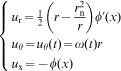
In this paper, it will be assumed that the part being welded can be approximated by a round tube under the combined loading of an axial compressive stress σ_x and a shear stress arising from frictional effects, denoted σ_xθ. The tube is assumed to be of length l with the shear stress acting at the origin; the boundary conditions are then (11) where P and A denote the axial load and the mating area respectively. The term τ₀ is the shear stress, which can be estimated from the study of deceleration curves such as curve 2 given in Fig. 4. To simplify the analysis and consistent with symmetry, the tube is modelled as a row of elements of thickness equal to that of the tube; in what follows both the stress component σ_x and σ_xθ are assumed to be homogeneous throughout the part.

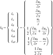
For the purposes of the present paper, the appropriate general velocity fields needed to describe the plastic deformation in the tube under the cylindrical coordinate system (Fig. 5) are then24 (12) where u_r, u_θ and u_x are the velocity components in the radial (r), circumferential (θ) and axial (x) directions respectively. The neutral radius is r_n, the average of the inner and outer radii. The term φ(x) is an arbitrary function used to describe the velocity field in the axial direction, and φ′(x) is the first order derivative of φ(x) with respect to x. It can be demonstrated that the above velocity fields satisfy the principle of volume conservation. The symmetry of the situation means that the velocity gradient in the circumferential direction is zero; then the components of the strain rate in the cylindrical coordinate system are25 (13) If we substitute the expression for u_θ given in equation (12) into equation (13), one sees that the shear strain rate is zero; hence, the corresponding stress component σ_rθ will also be zero. This is consistent with the tube remaining circular throughout the welding process.

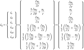
Next one needs to consider the flow behaviour of the material. Owing to the significant deformation occurring at high temperatures, the elastic portion of the strain will be small compared with the plastic strain; therefore it has been omitted from the calculations which follow. Hence, the Levy–Mises flow rule has been adopted as follows26 (14) where is the plastic strain rate tensor and S_ij is the deviatoric stress tensor. 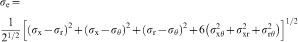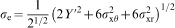The term is determined from (15) where is the effective plastic strain rate. The term σ_e is the effective stress; in the cylindrical coordinate system, it is26 (16) where σ_x, σ_r and σ_θ are the normal stresses acting in the axial, radial and tangential directions respectively, and σ_xr, σ_xθ and σ_rθ are the shear stress components. It can also be expressed by the corresponding deviatoric stress components, S_x, S_r and S_θ, as (17) where S_r, S_θ and S_x represent the deviatoric stress components in the radial, circumferential and axial directions respectively. The IN718 material being analysed is assumed to obey the von Mises yield criterion, so that (18) The term Y′ is the flow stress in uniaxial tension/compression, modified such that the effect of the shear stress components are excluded; its relationship with the actual uniaxial flow stress is (19) When the Levy–Mises flow rule of equation (14) is used, the deviatoric stress components corresponding to the approximating velocity field in equation (12) can be written as follows24 (20) where the σ_xr is the shear stress in the rox plane.

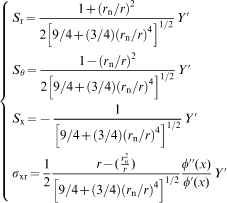
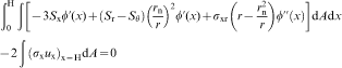
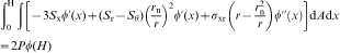
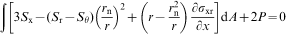
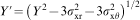
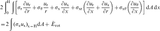
As φ(x) is an arbitrary function, σ_xr is still unknown in equation (20). It is estimated as follows, by making use of Hill's general method. 24 26 24,26,27 According to the principle of energy conservation, for the case of inertia welding of a round tube one has (21) where A represents the cross-sectional area and H is the height of the deformation zone in the heat affected zone (HAZ). The item in the left side of the equation is the energy dissipation rate. The first item in the right side of the equation is the work rate of the external compression load, the second item is the energy dissipation rate of the rotation energy. It is assumed that the kinetic energy of the rotating part is entirely consumed in the work done by the friction induced shear stress σ_xθ to generate heat. Hence (22) Then equation (21) becomes (23) We proceed as follows. Ignoring for a moment any influence of the shear stress component σ_xθ, the velocity component u_θ is taken as a constant to let σ_xθ be zero. Substitution of the velocity fields in equation (12) into equation (21) results in (24) This equation can be further written as (25) where P is the compression load calculated by (26) Integrating by parts to the third item in the left side of the equation (25) and noting that (27) and (σ_xr)_x = 0 = 0, equation (25) becomes (28) Since φ′(x) is an arbitrary function, we have (29) and (30) Equation (29) states the relationship of the stress components in the deformation zone from the perspective of the force equilibrium with respect to the external load P. This equation has been used to estimate the rate of change of the shear stress ∂σ_xr/∂x. As σ_xr is zero at the origin x = 0, the average value of σ_xr at each section can be worked out numerically.

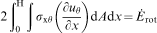
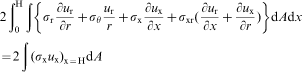
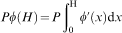
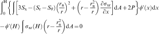
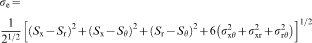
The effective stress σ_e can then be expressed as (31) where σ_xθ is the shear stress produced in the material to balance the torque produced from friction. Then according to the Levy–Mises flow rule, the axial compression strain rate is (32) In order to perform the mechanical calculation, the length of the tube is discretised with cylindrical elements which are arranged in a one-dimensional fashion along the axial direction. The length l of the tube which is modelled is 70 mm; it is partitioned into n subintervals of equal length Δx = l/n. The Δx is set to 0·05 mm. Since the length of each subinterval is small, the temperature within the each subinterval can be taken as constant over the length at each time step, without loss of accuracy. For each subinterval, the compression strain rate along axial direction, i.e. x direction is calculated according to equation (32). If the effective strain rate is known, the axial strain can be integrated along the length of the tube, and the displacement of the weldline (upset) calculated.

Constitutive equation used: Lambda model

To calculate the displacement of the weldline with equation (32), it is necessary to propose a constitutive relationship for the material during hot deformation. In the literature, many constitutive equations are available to describe the hot deformation behaviour of IN718.28^–32 In fact, the constitutive equations are not always consistent with each other, probably due to differences in composition, processing method and microstructure. Here, we have chosen to implement the lambda model proposed by Blackwell et al.,33 in which a microstructure related internal variable λ is used together with the Zener–Hollomon parameter Z. Compared with other models, for example, those proposed by Lin and Dean34 and Zhao et al.,30 the lambda model does not have a significant number of parameters and is relatively easy to implement. In fact, the formulae in paper by Blackwell et al.33 can be summarised succinctly as follows (33) where m, n and β are material constants, Y and ϵ_e are the flow stress and effective strain respectively, and k₁ is a scaling constant. The term λ is the microstructure related state variable parameter, which is set to an initial value of unity but which is allowed to evolve consistently with (34) where λ₀, q₀ and α are all material related constants. The Zener–Hollomon parameter used is defined according to (35) where is the effective strain rate, Q is an activation energy and R is the gas constant.

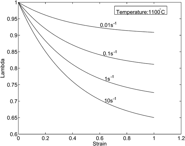
The parameters used in the lambda model to describe IN718's stress–strain relationship are summarised in Table 2. Figure 6 illustrates some of the stress–strain relationships which then arise; these are calculated from equation (33) for various values of T and , noting that λ needs to be updated at each ϵ_e. The value for λ varies between 0 and 1, within the ranges of the temperature and strain rate used in this simulation; in the calculations which follow its value is carried across as T and evolve, consistent with the state variable approach. As illustrated in Fig. 7, λ scales inversely with the flow stress, so that it is an internal variable which is related to the extent to which the microstructure resists hardening during hot deformation.

Figure 6

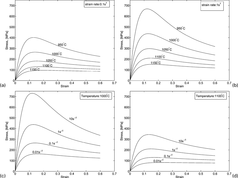
Prediction of stress–strain curves for IN718 from lambda model: at strain rates of a 0·1 s⁻¹ and b 1 s⁻¹; at temperatures of c 1000°C and d 1100°C

Figure 7

Variation of lambda with strain under various strain rate conditions

Table 2

Parameters used in lambda model

Alloy	k ₁	λ ₀	n	m	q ₀	α	β	Q/R
IN718	5·369×10⁻³	7·576	2·877	0·2522	−5·4354×10⁻²	2·487	18·78	59407

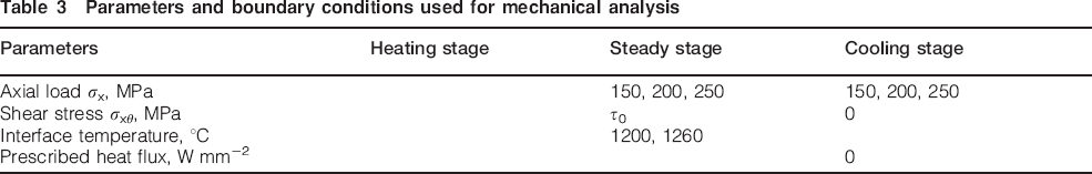
Parameters and boundary conditions used for mechanical analysis

In this study, a major goal is to analyse the influence of the shear stress σ_xθ developed due to frictional effects; as shown in Fig. 4, this becomes significant at the very last stage of welding and therefore needs to be accounted for. To simplify the calculation, the shear stress in each subinterval of the analytical model is assumed to be identical at each step, due to the balancing effect of the torque. The shear stress is also assumed not to change with the different temperatures assumed in the welding interface. The shear stress used in calculation is from curve 2 in Fig. 4, whose value is denoted as τ₀ in Table 3.

Table 3

Parameters and boundary conditions used for mechanical analysis

Parameters	Steady stage	Cooling stage
Axial load σ_x, MPa	150, 200, 250	150, 200, 250
Shear stress σ_xθ, MPa	τ ₀	0
Interface temperature, °C	1200, 1260
Prescribed heat flux, W mm⁻²		0

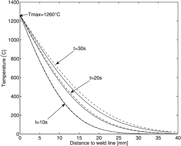
To study the sensitivity of the upset to the process parameters, different values of parameters such as compression stress and interface temperature were assumed in the calculations. Throughout, the upset arising during the heating stage has not been considered because it has been found to be very small. Looking at the amount of deformation seen within the first 3·5 s of the steady stage, one can see that upset value will be negligible for a weld interface temperature of 1200°C (Fig. 8a) and less than 5 of the final upset for a temperature of 1260°C (Fig. 8b). Therfore, any deformation happening during the heating stage, keeping in mind that the temperature distribution in this stage in the weld area will be narrower than during the steady stage, and with lower maximal temperature, therfore, any upset generated will be less than 5 of the final upset and can reasonnably be neglected.

Figure 8

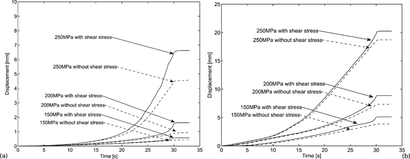
Prediction of evolution of upset by analytical model with interface temperature assumed to be a 1200°C and b 1260°C

The time for steady stage is taken to be 30 s. The compression stress is varied from 150 to 250 MPa. The calculation conditions used for the calculations are summarised in Table 3.

The stages of the calculation of the upset in the mechanical analysis can be summarised as follows:

the calculation of the temperature field through the thermal analysis of the section on ‘Thermal analysis: modelling of heat transfer’

the calculation of deviatoric stress S_r, S_θ and S_x through equation (20) under the assumed velocity field

iii

the determination of shear stress σ_xr through equation (29) using numerical integration

the calculation of the flow stress through equation (31)

the determination of the effective strain rate by substitution of values for temperature, effective stress and strain into the constitutive equation: the lambda model

the determination of the axial strain rate by equation (32)

vii

calculation of the strain in each subelement and integration of it along the length of the tube

viii

repetition of the above as necessary, until the simulation is complete.

FEM model of inertia welding

2½D element for friction welding

The analytical model makes some major assumptions and it is of interest to compare its predictions with those made using the FEM. For this purpose, the commercial FEM code DEFORM-2D has been used, in which a special 2½D axisymmetric element is available to simulate inertia welding; this allows torsional effects to be treated. 35 35,36 The basis for the FEM is the variational method. 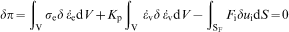It states that among all admissible velocity u_i that satisfy the boundary conditions, the solution velocity field makes the following functional a minimum value26 (36) where is the volumetric strain rate, F_i is surface traction over the surface S_F and K_p is a penalty constant. In DEFORM, to describe the torsional effects while keeping the 2D axisymmetric condition for computational efficiency, it is assumed that there is no velocity gradient in the circumferential direction for the velocity fields involved in inertia welding.35 The velocity field is then where u_r, u_x and u_θ are the velocity components in the radial (r), axial (x) and circumferential (θ) directions respectively. The related strain rate tensor is as follows (37) The corresponding deviator stress tensor can be calculated with Levy–Mises flow rule, as given in equation (14). So compared with a conventional axisymmetric model, two further shear stress components, σ_rθ and σ_xθ, are non-zero and are determined during the calculations, in addition to the σ_rx required for a regular axisymmetric calculation. The non-standard element (a so called 2½D element 35 35,36) is used for purpose.

Calculation conditions

The FEM mesh used in this study is shown in Fig. 9. Only half of the section of the tube is illustrated because of the axial symmetry. It contains 1047 quadrilateral elements and 1126 nodes, with the mesh designed to be much finer close to the weld interface in order to capture the large plastic strain and steep temperature fields expected there. The size of the smallest element is around 0·4 mm, and the largest one is around 1 mm. This mesh was chosen after demonstrating that the results were unaltered when finer meshes were used, e.g. one with 10 000 quadrilateral elements, with a smallest element of only 0·03 mm. Our findings are consistent the results of others. For example, Bennett et al. studied the effect of mesh size for the simulation of inertia welding and noted that an element size of ∼0·3 mm at the welding interface was fine enough to ensure accuracy.21 D'Alvise also held that a mesh size of 0·4 mm is reasonable.36

Figure 9

Mesh used for FEM simulation, containing 1047 elements and 1126 nodes

To enable a fair comparison between the FEM model and the analytical one, the simulation of the inertia welding by the FEM method was divided into three steps consistent with the three stages of the welding process, i.e. the simulation of the heating stage, the steady stage and the cooling stage. The thermal properties of IN718 employed were the same as those used in the analytical analysis, while the constitutive relationship is described with the lambda model and input into the code via a fortran subroutine. The boundary conditions used in the FEM model are also the same as those used in the analytical calculations; furthermore, the heating effect of friction in the welding interface is simulated using a constant heat flux during the heating stage and a fixed temperature at the weldline during the second stage, as before. The effect of convection and radiation is not considered in the thermal simulation carried out by FEM, as for the analytical model. A constant compressive stress σ_x is applied throughout.

To simulate torsional effects, the interfacial shear stress σ_xθ used in the FEM model is set up with a Coulomb friction model, in which the friction coefficient is assumed to be a function of time. The values of friction coefficient under different compression loads are set to be consistent with the values of the shear stress of curve 2 of Fig. 4. So if the compression load is 250 MPa, for example, the corresponding friction coefficient is then as given in Fig. 10. This allows a fair comparison between the FEM and the analytical models, as the shear stresses generated by friction in the FEM model will be identical to those applied in the analytical model.

Figure 10

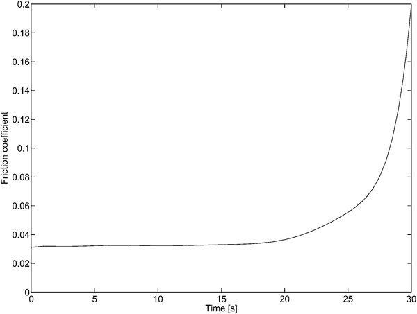
Variation of friction coefficient used in FEM simulation under load of 250 MPa

Results and discussion

Thermal results

Temperature profiles at different stages

Figure 11a illustrates the temperature profile in the workpiece during the heating stage, assuming a heat flux of 5 W mm⁻²; this is a reasonable figure for this first part of the process. For this flux, one can see that a temperature of 1260°C (the melting temperature of IN718) is reached in about 3·5 s. After 5 s, it reaches a temperature of 1500°C, which is far beyond the melting point and therefore physically unrealistic, since it is usually believed that no gross melting occurs during the inertia welding process. Hence, after the melting point is reached (i.e. at t = 3·5 s for a flux of 5 W mm⁻²), one prescribes instead a fixed temperature, which is taken to be the melting temperature of 1260°C. Figure 11b illustrates the temperature distribution during the second stage. One can see that the temperature gradient decreases gradually with increasing holding time. When the relative motion at the joint ceases, heat is no longer generated there and the third cooling stage begins. Figure 11c illustrates the temperature distribution made at various times thereafter.

Figure 11

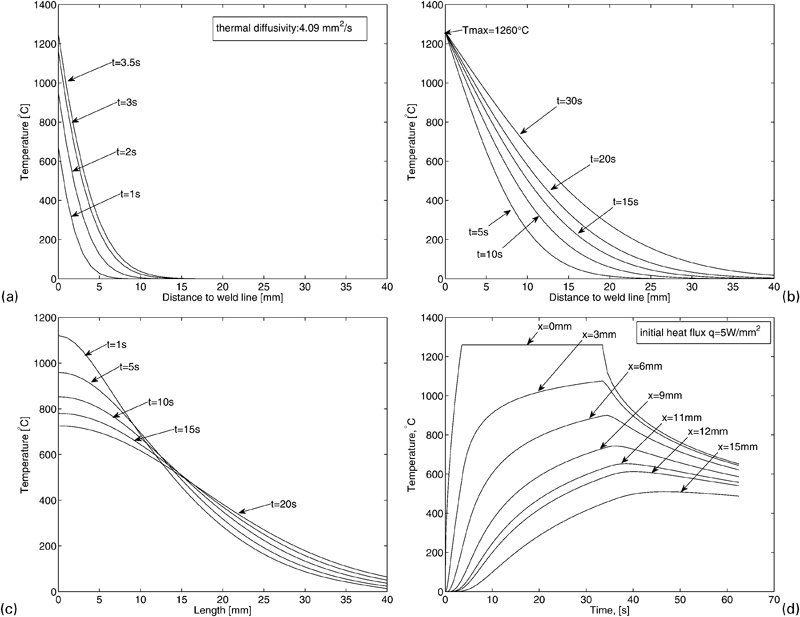
Thermal prediction of analytical model: a temperature profile during heating stage (q = 5 W mm⁻²); b temperature profiles during steady state stage; c temperature profiles during cooling stage; d predicted thermal history at different points away from weld interface

The thermal histories of regions close to the weldline is of interest, since these will control the microstructure and properties exhibited (Fig. 11d). Once again, the heat flux is taken to be 5 W mm⁻² for the heating stage; after 3·5 s the welding interface is kept at 1260°C for 30 s, and cooling follows. One can see that the region near the welding interface, for example at the point x = 3 mm, reaches the highest temperature at the end of the heating stage, i.e. t = 33·5 s, while for the region further from the weldline, for example, at the points x = 6 mm and x = 9 mm, the highest temperature appears during the cooling stage. This is because of the heat conducted from the zone near the weldline with the higher temperature. As the microstructure of IN718 is altered when exposed to a temperature higher than 650°C,1 if the HAZ for welded IN718 is defined as the zone which experiences a temperature higher than this value, the width of the HAZ is predicted to be about 11 mm for these conditions.

Heat flux study

It is important to consider how the magnitude of the heat flux influences the time taken for the melting temperature to be reached. From equation (8), the temperature at the weldline during the heating stage is 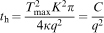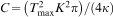(38) where the symbols have the same meaning as those in equation (8). If the highest temperature reached in inertia welding is defined as T_max, from equation (38), the relationship between heat flux value q and time t_h needed for temperature at the welding interface to reach T_max is given by (39) where can be taken as a constant. Equation (39) indicates that the heating time t_h is inversely proportional to the square of heat flux q. If T_max is assumed to be 1260°C, the relationship between t_h and q for IN718 is as given in Fig. 12a.

Figure 12

Effects of heat: a relationship between heating time t_h and heat flux q for IN718; b the effective heat fluxes for whole welding process

In practice, different heat fluxes can be encountered due to different parameters used, e.g. axial load and rotation speed. Here, the effect of altering the value of the heat flux has been studied with the assumption that the highest temperature reached remains unchanged, at 1260°C. The relationship between the heat flux q and the temperature profile T(x,t) is as follows (40) Finally, one can determine the heat flux needed at the interface (x = 0) to maintain a value equivalent to the melting temperature during the second stage of the process. The results are shown in Fig. 12b, in which the effective heat flux for the complete process is given. In the calculations, the total time span for the first two stages was assumed to be the same, at 30 s. It is found that the time for the heating stage varies considerably depending upon the initial value of the heat flux. When the temperature reaches the highest point, the effective heat flux curve drops quickly. As time goes by, the effective heat flux curves for different processes gradually coincide, which means that the temperature profiles are gradually becoming coincident as the time in the steady stage increases.

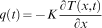
Peak temperature distribution

The distribution of peak temperatures is important since this will influence microstructural changes markedly. Various initial heat fluxes have been studied. The results confirm that the profiles for peak temperature distribution change little if the holding time for the steady stage is long enough. For example, in Fig. 13a, the total time for the first two stages is 30 s and the curves representing the peak temperature distribution along the rod are nearly the same. When the initial heat flux is kept constant, for example, 5 W mm⁻², and the holding time for steady stage varies, the corresponding peak temperature curves are quite different. In Fig. 13b, the peak temperature distribution curves under different holding times, from 5 to 30 s, is presented. The highest temperature at the weldline is assumed to be 1260°C. If we define the HAZ as temperature above 650°C for IN718, then the width of the HAZ after holding for 5 s is about 5·3 mm, while holding for 30 s, the width of the HAZ is 11 mm. So compared with the initial heat flux, the peak temperature distribution is more sensitive to the holding time during the steady stage.

Figure 13

Peak temperature curves: a peak temperature curves for various initial heat fluxes; b peak temperature curves for various holding times during steady stage

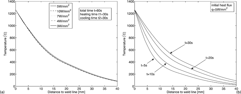
Comparison of thermal results from FEM and analytical method

The temperature profiles at different times as predicted by both the analytical and FEM models are illustrated in Fig. 14. The temperature profiles from the FEM model are quoted at the average of the inner and outer radii of the tube. From the graph, one can see that the temperature fields from the two methods are quite similar at the early stage of welding. For example, the two estimates of the temperature profiles are more or less identical at a time of 10 s. At later times, a greater difference is apparent, with the temperatures predicted from analytical method being greater than those from the FEM. We believe these inconsistencies to be explained by differences in the axial shortening predicted by the two models, as will become apparent.

Figure 14

Comparison of temperature profiles from analytical model and FEM model: dashed lines represent analytical results; solid lines are from FEM

Mechanical results

Upset predictions from analytical and FEM models

Figure 8 illustrates how the analytical model predicts the total upset to vary with time, for interface temperatures of 1200 and 1260°C. One can see that the rate of change of the total upset with time increases steadily until eventually it reaches a plateau; this is due to the onset of the cooling stage when the interfacial temperature drops rapidly. Consequently, the upset curves become flat because plastic deformation is then severely restricted. The influence of the shear stress was also studied, as illustrated in these graphs. The shear stress refers to the shear stress component σ_xθ, which is the result of the torque produced from the friction at the welding interface. The solid lines represent the upset predicted with both the shear stress and the compression stress included in the simulation. The dashed lines represent the corresponding curves when the shear stress is excluded. The results demonstrate that the combined action of the compression stress and the shear stress increases the upset value significantly; moreover, the slope of the upset curve increases markedly at the end of the steady stage, an effect which is due to the increase in the shear stress which is occurring towards the later part of the process. The effect of the interface temperature is also very significant; the upset increases from 6·6 to 20 mm when the interface temperature rises from 1200 to 1260°C under a compression load of 250 MPa.

The results predicted by the FEM model are given in Fig. 15; as for the analytical solution, the impact of temperature on the upset value is considerable. Once again, one can see that the predicted values for the upset increase markedly when the temperature increases from 1200 to 1260°C. The shear stress's influence is also significant. In Fig. 15, the solid lines represent the upset curves calculated with the shear stress, and the dashed lines correspond to those without shear stress. The values of upsets of the curves representing the combined action of compression stress and shear stress are always higher than those under the sole action of compression stress.

Figure 15

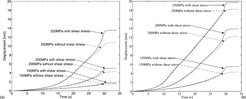
Prediction of evolution of upset by FEM model with interface temperature assumed to be a 1200°C and b 1260°C

Comparison between FEM and analytical models

The FEM method presents a number of advantages for the present analysis, namely,

a rigorous analysis of the stress tensor under the 2 ½D symmetry which is prevalent

a better capability for the prediction of the geometry of the flash region, which will influence the accuracy by which the total upset can be predicted

iii

a more rigorous coupling of the thermal and mechanical analyses such that effects such as adiabatic heating can be accounted for.

It is of interest to compare the results from the analytical and FEM models in the light of the above (Figs. 8 and 15). Broadly speaking, the forms of the predictions are broadly consistent, although the absolute values of predicted upset are different. Both models predict that the upset rises with the increase of the compression load. Most of the results from the analytical one are smaller than their counterparts from the FEM model. Probably this is due to the lack of the consideration of the flash formation in the analytical model. Thus, elements which are severely deformed plastically are accumulated near the weldline in the analytical model, when in reality they can be expelled in the radial direction so that a flash is formed. In the FEM model, elements with large strain are expelled out to form flash, leaving room for the following elements to near the welding interface to undergo more drastic thermo-mechanical deformation, which will accelerate the upset rate.

In analytical model, the upset is more sensitive to the change in external load. This may be due to the differences in the details of the temperature calculation. In the analytical model, the thermal analysis is one-dimensional, but in the FEM model, the results are two dimensional. The influence of the flash forming on the temperature field is taken into account in the FEM model. Further, the effect of the load on the temperature distribution is well represented in the FEM model. A shortening effect on the width of the HAZ will occur. This means that there is a tendency for a narrowing of the deformation zone with an increase in the load, which may impede the plastic deformation. In the analytical model, this effect is not included, which may explain the difference.

On effect of adiabatic heating

A final point is that, apart from the heating arising from friction, adiabatic heating from plastic deformation is not considered in the analytical model. To examine this assumption, the FEM model has been run both with and without the adiabatic heating effect included in the calculation (Fig. 16). The compression stress is taken to be 150 MPa and the temperature at the interface is assumed to be 1260°C. One can see that any error arising from the neglect of adiabatic heating is small, <3. If we define the region whose temperature is above 650°C to be the HAZ, the width of HAZ for the case with adiabatic heating is around 9·5 mm, while the width of HAZ for the one with no adiabatic heating is around 9·6 mm. Thus, it would appear that any adiabatic heating due to plastic deformation has only a small effect; its contribution is very small compared with the frictional heating occurring at the welding interface. Any differences between the analytical and FEM models are therefore not due to this effect.

Figure 16

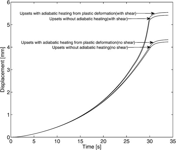
Effect of adiabatic heating from plastic deformation in FEM model

Size of HAZ

The analytical model predicts a HAZ of 11 mm and FEM predicts about 9·5 mm. These two values seems a bit large, and looking at the literature Huang et al.37 have reported HAZ of about 5 mm in IN718, although it was in the case of dissimilar weld (720Li to IN718). The differences between predicted values and the value reported in this experimental work are probably due to the heat losses by radiation and convection that have been neglected in our models.

Another limitation of our analytical model, which is partially responsible for the difference between the analytical model and FEM model results, is that the thermal calculation is not coupled with the mechanical calculation. This is not an issue as long as the deformation rates in the mechanical model are small, but when experiencing the large deformation rate seen at the end of the welding process, the effect of the deformation on the thermal field is no longer negligible, and the mass transfer towards the weldline will reduce the HAZ size.

Discussion

The results presented above raise some interesting questions, particularly concerning the behaviour of the material in the vicinity of the joint during processing. In this paper, it has been assumed that the melting point of the material represents an upper limit for the temperature experienced; however, throughout the history of friction welding, the question of the precise interface temperature and whether melting occurs on a gross scale has been unanswered and indeed controversial.38 Many researchers seem to be of the opinion that melting does not occur. 11 13 38 11,13,38,39 However, it is hard to explain why the friction coefficient in friction welding can be as low as 0·02 during its steady stage,40 which is equivalent to a metal plate slipping on ice. The friction coefficients applicable to metal–metal contact are usually much higher, so it seems possible that some liquid is acting as a lubricant during friction welding.41 Furthermore, the rapid heating rate during the heating stage of friction welding also suggests that at least some localised melting might be expected. Cheng assumed a molten layer in the weldline in a FDM model of friction welding, with the temperatures computed agreeing well with the experimental data.12 Midling and Grong reported there was a molten layer in friction welding of aluminum alloys to Al–SiC metal matrix composites.7 Soucail et al. also reported an incipient melting phenomenon in inertia welding of Astroloy.42

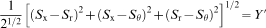
The main reason given by the researchers who are against the possibility of any melting occurring is that any liquid layer would be expected to be expelled out from the weld under the forces generated, should it indeed be present; little evidence for this is found. The modelling results shed some light on this, and indicate that there are some factors which might mean that a semimolten zone may in fact be held within the vicinity of the joint, in a stable fashion. First, it has been demonstrated that the temperature gradient near weldline is very steep, so that the thickness of any liquid-like layer at the weldline will be very small. Second and perhaps more importantly, one should consider the state of stress of the material at the weldline which, as shown in this paper, is in fact strongly influenced by the fact that the temperature gradient is steep. A thin soft layer existing at the weldline will indeed be expelled radially if the speed of rotation is too high, but one has to consider also the significant hydrostatic component of stress which is generated during the process which should act to mitigate this. Failure to account for this effect will lead to an oversimplified model, and a wrong interpretation of the stress state present. To see this, consider the round tube analysed in this paper; considering the combined loading of the compressive axial stress and the shear stress arising from frictional effects (no other stress component being accounted for) the compressive strain rate along the axial direction would then be calculated (incorrectly) according to (41) where σ_x is the nominal axial compression stress. Compare equation (41) with the correct form as used in this paper, given in equation (32). During our research, it has been found that use of equation (41) leads to predicted values of the upset very substantially greater than those observed in practice. The cause for this is as follows. During inertia friction welding, material in the vicinity of the weldline is very soft, while the externally applied compressive stress is normally in the range of several hundred MPa, so material at the weldline will have a very high strain rate under the action of the applied axial pressure. For instance, given the constitutive equations and data used here, the strain rates for IN718 under different temperatures and pressures are as shown in Fig. 17. The initial strain in this graph is set to be 0·1. It is seen that the strain rate of IN718 at a temperature of 1260°C under the uniaxial compression pressure of 250 MPa can be as high as 250 s⁻¹. That means the soft metal at the welding interface will be deformed readily in the predictions, which is not what actually happened in practice. This result seems to be consistent with the view of many researchers that the temperature at the mating surface cannot be too high; otherwise, the metal near mating surfaces will be squeezed out quickly due to the very low flow stress of metal at that temperature. Sluzalec even held that the limiting steady state temperature in the joint cannot be higher than the temperature at which the yield point of the material is equal to the pressure used in the experiment.15 However, if Sluzalec's claim is correct, the friction stress during steady state stage would never be low enough to be in the range of 10 MPa or even less since the friction stress is deemed equal to the shear strength of the metal at the welding interfaces during steady state stage of friction welding, which should also be in the range of several hundred MPa.40 And from the considerations given above, it seems plausible that the holding effect of the hydrostatic stress is the reason for the existence of the soft material there. These ideas are supported by the results from the FEM model. Figure 18 is the stress fields distribution during inertia welding from the FEM model. One can see that all three normal stress components, i.e. the normal stress components in axial, radial and hoop direction, have high negative values near the weldline, with the result that there is a band of high hydrostatic stress there. The presence of this significant hydrostatic component of the stress field and its implications does not seem to have been realised by previous authors.

Figure 17

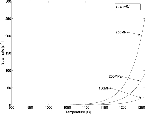
Variations of strain rates under different temperatures and uniaxial pressures

Figure 18

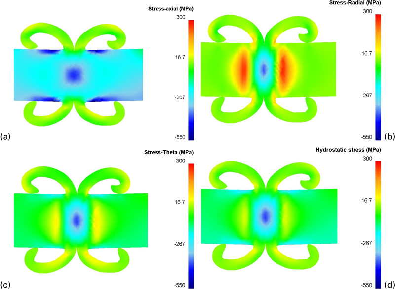
Stress distribution in inertia welding: a normal stress in axial direction; b normal stress in radial direction; c normal stress in hoop direction; d hydrostatic stress distribution

A final point relates to the precise value of the interfacial temperature assumed for the IN718 superalloy. In this paper, an upper limit of 1260°C has been assumed. Some researchers believe that this is the point at which IN718 just starts to melt. 43 43,44 But according to Lewandowski and Overfelt,45 IN718 is already in a semisolid state at this temperature; solid phases are in the majority, but a small fraction of liquid lies intergranularly which might ease the deformation greatly.45 So the assumption of a temperature of 1260°C in this study may in fact be very close to the reality. The presence of this mushy zone would mean that there is some liquid in the weldline which acts as lubricant to reduce the friction greatly during friction welding.

Conclusions

The following conclusions can be drawn from this work:

A thermal–mechanical analytical model, with the adoption of the lambda model to describe the constitutive relationship of a nickel based superalloy at high temperatures, has been built to simulate inertia friction welding; particular emphasis has been paid to IN718.

The presence of the shear stress is found to enhance the upset caused by the process; its rapid increase during the last seconds of welding can influence the upset markedly, and this needs to be accounted for if the predictions are to be accurate.

The upset experienced is found to be very sensitive to the temperature assumed at the weld interface. A small rise in the interface temperature leads to a significant increase in the axial shortening.

The effect of adiabatic heating from plastic deformation is small compared with the heating effect from friction welding; thus it is reasonable for this to be neglected.

To maintain a constant temperature at the contact section, the effective heat flux must decrease with increasing time.

The width of the HAZ is sensitive to the time spent at the flash forming stage, i.e. the steady state stage. The higher the holding time, the wider the HAZ. So the holding time will influence the joint quality markedly. The width of the HAZ also changes with the load: the higher the compression stress, the narrower the HAZ.

Given suitable parameters for the constitutive, it is demonstrated that the analytical model gives a first order estimate of the upset expected during inertia welding. Given its speed of application, it is useful, e.g. for the rapid prediction of the temperature gradients expected and to aid in the design of FEM meshes.

During inertia friction welding of superalloys, it seems possible that a semi-solid slurry-like layer can exist close to the weldline, which is held in place by the high hydrostatic stress state which has been shown to be present there.

Footnotes

Acknowledgements

One of the authors (LY) is grateful for financial aid from Department of Metallurgy and Materials, University of Birmingham and the Overseas Research Student Awards Scheme (ORSAS). The authors are grateful to Professor J. Brooks from the AFRC, University of Strathclyde, for his help with the constitutive model used. The authors also thank Dr F. Daus from the University of Birmingham for helpful discussions.

References

Sims

C T

, Stoloff

N S

, Hagel

W C

, ed (eds.): ‘Superalloys II’; 1987, New York, John Wiley & Sons Inc.

Reed

: ‘The superalloys: fundamentals and applications’; 2006, Cambridge, Cambridge University Press.

Schafrik

, Walston

:in ‘Superalloys 2008’(, Reed

R C

, et al..), 3–9; 2008, Warrendale, PA, TMS.

‘Welding – friction welding of metallic materials’, BS EN ISO 15620:2000, BSI, London, 2000.

O'Brien

, ed (ed.): ‘Welding handbook: welding processes’; 1991, Miami, FL, American Welding Society.

Wang

: Weld Res. Counc. Bull. , 1975, (204), 1–22.

Midling

, Grong

: Acta Metall. Mater. , 1994, 42, (5), 1595–1609.

Rykalin

, Pugin

, Vasil'Eva

: Weld. Prod. , 1959, 6, 42–52.

Healy

, Mcmullan

, Bahrani

: Wear , 1976, 37, 265–278.

10.

Francis

, Craine

: Int. J. Heat Mass Transfer , 1985, 28, 1747–1755.

11.

Dave

, Cola

, Hussen

: Weld. J. , 2001, 80, (10), 246s–252s.

12.

Cheng

: Weld. Res. Suppl. , 1962, 41, 542–550.

13.

Wang

, Nagappan

: Weld. Res. , 1970, 49, 419s–426s.

14.

Maalekian

, Kozeschnik

, Brantner

, Cerjak

: Acta Mater. , 2008, 56, (12), 2843–2855.

15.

Sluzalec

: Int. J. Mech. Sci. , 1990, 32, 467–478.

16.

Moal

, Massoni

: Eng. Comput. , 1995, 12, (6), 497–512.

17.

, Duan

, Du

: Weld. J. , 2003, 82, (3), 65–70.

18.

D'Alvise

, Massoni

, Walloe

: J. Mater. Process. Technol. , 2002, 125–126, 387–391.

19.

Wang

, Preuss

, Withers

, Baxter

, Wilson

: Metall. Mater. Trans. B , 2005, 36B, 513–523.

20.

Zhang

, Zhang

, Liu

, Zhang

, Zhu

, Qu

: Sci. Technol. Weld. Join. , 2006, 11, (6), 737–743.

21.

Bennett

, Hyde

, Williams

: Proc. IMechE Part L: J. Mater.: Des. Appl. , 2007, 221L, (4), 275–284.

22.

Hill

, Dewynne

: ‘Heat conduction’; 1987, New York, Blackwell Scientific Publications.

23.

Carslaw

, Jaeger

: ‘Conduction of heat in solids’; 1959, Oxford, Oxford University Press.

24.

Lahoti

, Kobayashi

: Int. J. Mech. Sci. , 1974, 16, 521–540.

25.

Chakrabarty

: ‘Theory of plasticity’; 1987, New York, McGraw-Hill Book Company, Inc.

26.

Kobayashi

, Oh

S.-I

, Altan

: ‘Metal forming and the finite-element method’; 1989, Oxford, Oxford University Press.

27.

Hill

: ‘Mathematical theory of plasticity’; 1950, Oxford, Clarendon Press.

28.

Zhang

, Gao

, Zhuang

, Zhong

: Metall. Mater. Trans. A , 1999, 30A, (10), 2701–2712.

29.

Dandre

, Roberts

, Evans

, Reed

: Mater. Sci. Technol. , 2000, 16, (1), 14–25.

30.

Zhao

, Guest

, Tin

, Cole

, Brooks

, Peers

: Mater. Sci. Technol. , 2004, 20, (11), 1414–1420.

31.

Medeiros

, Prasad

, Frazier

, Srinivasan

: Mater. Sci. Eng. A , 2000, A293, (1–2), 198–207.

32.

Narayana Murty

, Nageswara Rao

, Kashyap

: Int. Mater. Rev. , 2000, 45, (1), 15–26.

33.

Blackwell

, Brooks

, Bate

: Mater. Sci. Technol. , 1998, 14, 1181–1188.

34.

Lin

, Dean

: J. Mater. Process. Technol. , 2005, 167, (2–3), 354–362.

35.

Lee

, Samant

, Wu

, Srivatsa

: ‘Finite element modeling of inertia welding processes’, Proc. Conf. NUMIFORM 2001, 1095–1100; 2001, Rotterdam: Balkema.

36.

D'Alvise

: ‘Development of a finite element model for the simulation of the inertia friction welding process between dissimilar materials’, PhD thesis, L'Ecole Nationale Superieure Des Mines De Paris, Paris, France, 2002.

37.

Huang

, Li

, Preuss

, Karadge

, Bowen

, Bray

, Baxter

: Metall. Mater. Trans. A , 2007, 38A, 1608–1620.

38.

Maalekian

: Sci. Technol. Weld. Join. , 2007, 12, 738–759.

39.

Rich

, Roberts

: Met. Constr. Br. Weld. J. , 1971, 2, 93–98.

40.

Daus

: ‘Process, microstructure and property relationships in dissimilar nickel base superalloy inertia friction welds’, PhD thesis, University of Birmingham, Birmingham, UK, 2009.

41.

Blau

P J

, Henry

S D

, Davidson

G M

, Zorc

T B

, Levicki

D R

, ed (eds.): ‘ASM handbook’, Vol. 18, ‘Friction, lubrication and wear technology’; 1992, Materials Park, OH, ASM International.

42.

Soucail

, Moal

, Naze

, Massoni

, Levaillant

, Bienvenu

:in ‘Superalloy 1992’(, Antolovich

S D

, et al..), 847–856; 1992, Warrendale, PA, TMS.

43.

Betteridge

, Heslop

, ed (eds.): ‘The Nimonic alloys, and other nickel-base high-temperature alloys’; 1974, London, Edward Arnold.

44.

Mills

: ‘Recommended values of thermophysical properties for selected commercial alloys’; 2002, Cambridge, Woodhead Publishing Limited.

45.

Lewandowski

, Overfelt

: Acta Mater. , 1999, 47, 4695–4710.