Determination of optimal location to monitor temperature in low pressure die casting process

Abstract

Controlling and eliminating defects, such as macroporosity, in castings is a continuing challenge that manufacturers must continually address. Since the encapsulation of liquid regions by a solid shell and subsequent formation of macroporosity cannot be detected during casting, the die temperature, which is routinely measured, has been used as an indirect indicator of this defect. A finite element model has been developed to predict the evolution of temperature as well as the volume of encapsulated liquid in a casting with a high propensity to form macroporosity. The boundary conditions in the model were iteratively adjusted until the temperature predictions matched the experimental data for a variety of operational conditions. A model based methodology has been developed to analyse the correlation between the die temperature and the encapsulated liquid volume. This methodology is employed to assess the suitability of different in-cycle die temperatures for use as indicators of macroporosity formation, and to help determine the optimal location to monitor temperature for the purpose of minimising macroporosity.

Keywords

Low pressure die casting Finite element model Macroporosity Optimisation Correlation

Introduction

The automotive industry continues to search for and to exploit opportunities to replace steel and cast iron components or assemblies with light weight aluminium castings. High volume casting methods that operate in a batch mode where parts are produced cyclically, such as low pressure die casting (LPDC), have facilitated this conversion.1,2 The evolution of the LPDC process and its development as a major manufacturing process have been discussed by a number of authors.3^–5 Currently, the LPDC process plays an increasingly important role in the foundry industry as a low cost and high efficiency precision forming technique with new applications beyond its typical use in the production of automotive wheels.1 In the LPDC process minimising defects, such as macro- and microporosity, is a continuing production challenge since these defects are the main source of rejected castings due to their deleterious effects on the mechanical properties and surface quality of cast components. In the case of macroporosity, the current philosophy to reduce its formation is to promote directional solidification and thereby eliminate hot spots. In practice, this can be accomplished by die structure design6 and the execution of a preset casting cycle that does not vary from cycle to cycle, e.g. using programmable logic controllers.7 Although straightforward to implement, this open loop (uncontrolled) approach to operating the process lacks the ability to adjust to variability in the casting process, resulting in the defective product during common process variations and disturbances, such as changing incoming metal temperature or variability in the amount of time that a die is open at the end of a casting cycle. To respond to process variability and mitigate its negative effects, advanced process control methodologies designed for other manufacturing systems may be adapted to dynamically adjust the operational parameters of a casting process.

The ability to identify and quantify a particular defect, such as the volume of macroporosity formed during casting, is a prerequisite for implementing an advanced control methodology. However, the inline characterisation of macroporosity in a casting process is a major challenge for producers and researchers. Although non-destructive measurement techniques, including ultrasonic inspection and X-ray imaging,8^–10 may be used to assess casting quality, the use of these methods in an industrial setting to characterise macroporosity is costly and the results tend to be qualitative rather than quantitative. Additionally, the time delay associated with performing and processing the measurement will adversely affect the performance of an advanced control method. Liquid encapsulation, a precursor to the formation of macroporosity, occurs when a volume of liquid becomes isolated by the formation of a solid (or near solid) shell at or below a critical temperature. The formation of macroporosity in a casting may thus be directly related to its temperature history during solidification.11 The temperatures in the casting may in turn be related to die temperatures and used as an indirect indicator of macroporosity.

In this study, a mathematical model of an LPDC process has been developed to act as a ‘virtual process’ for use in developing and testing an advanced process control solution. The mathematical model predicts the cyclic temperature variation in the casting and die of an experimental LPDC casting process as well as estimating the extent of macroporosity formation and has been validated by comparison with experimental data. A model based methodology to analyse the correlation between the die temperature and the volume of encapsulated liquid has been developed. It is then used in determining the optimal location to monitor temperature in the experimental die. Determining the optimal location and assessing alternate locations to monitor temperatures in a die are important steps in the development of a casting process and its control methodology.

Model development

In this research, a computer based transient heat conduction model of a solidifying LPDC casting and die was developed to predict the temperature variation throughout the casting process. The use of a casting model versus performing plant trials provides advantages: a model is inherently flexible allowing a wide variety of operational conditions to be evaluated at a model at a relatively low cost compared to plant trials. Also, a model can provide temperature information at any (and/or all) locations within the model domain whereas measured temperature data are limited to locations where thermocouples have been installed in a plant trial. The mathematical model developed in this study was implemented in the commercial finite element package, ABAQUS. The geometrically simple demonstration die, shown in Fig. 1, was designed for this study to provide a test platform to assess further control strategies. Contrary to production castings, this casting process was designed with the goal of producing easily quantifiable defects, specifically two regions of macroporosity.

Figure 1

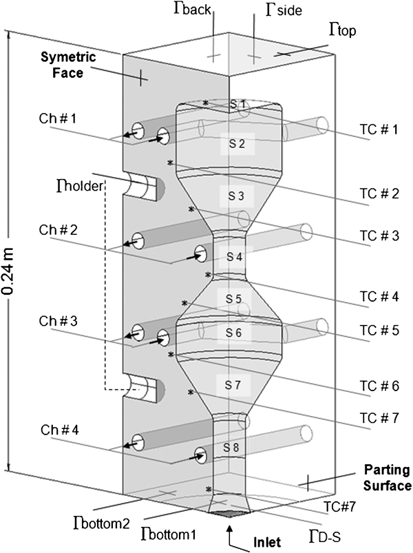
Schematic of 1/4 section of die with cooling channels, thermocouples locations and interior surface partitions marked

The model is based on the three-dimensional transient heat conduction equation (1) where T is the temperature (°C), k is the thermal conductivity (W m⁻¹ °C⁻¹), ρ is the density (kg m⁻³), C_p is the specific heat (J kg⁻¹ °C⁻¹), t is the time (s) and Q is the volumetric heat source term (W m⁻³) associated with the latent heat of solidification applied in the casting when appropriate, i.e. during the liquid to solid phase change, and x, y and z are the coordinates (m). To solve equation (1) for temperature using the finite element method requires the definition of geometry, material properties, initial conditions and boundary conditions.

Geometry

By taking advantage of symmetry, the geometry of the casting and die were reduced to a 1/4 section to shorten computation times. The die geometry in the model with overall dimensions of 240×80×80 mm is presented in Fig. 1. Four pairs of cooling channels, also shown in Fig. 1, were located at different heights in the die. In each pair, coolant (air or water) enters the die along the channel closest to the casting and returns through the other channel. The geometry of the casting and die was meshed with four node linear tetrahedral elements with minimum element edge lengths of 4 and 7 mm repsectively. The mesh contains 11 773 nodes and 50 115 elements. A refined mesh was developed to assess the sensitivity of the model predictions to increased mesh density. The temperatures predicted by the model for the two meshes varied by less than 1°C overall indicating that the use of the refined mesh was not necessary.

Thermophysical properties

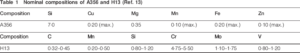
The die was fabricated from H13 tool steel and A356 aluminium alloy was used to produce the castings. The nominal compositions of these alloys are given in Table 1. The thermophysical properties of A356 and H13, including thermal conductivity, specific heat, density and latent heat (where necessary), used in the model were based on a variety of literature sources and are given in Table 2. During the liquid to solid phase transformation, the latent heat of solidification is released linearly in a series of segments based on the evolution of fraction solid as in Ref. 2. Primary solidification of A356 starts at 610°C and continues until 568°C when eutectic solidification begins.12 Since the microstructure of A356 is composed of 50 primary α and 50 eutectic phases, the latent heat released during solidification has been equally partitioned in these two ranges.2

Table 1

Nominal compositions of A356 and H13 (Ref. 13)

Composition	Si	Cu	Mg	Mn	Fe	Zn
A356	7·0	0·20 (max.)	0·35	0·10 (max.)	0·20 (max.)	0·10 (max.)
Composition	C	Mn	Si	Cr	Mo	V
H13	0·32–0·45	0·20–0·50	0·80–1·20	4·75–5·50	1·10–1·75	0·80–1·20

Table 2

Thermophysical properties for A356 and H13 used in thermal model14

Material	T/°C	k/W m⁻¹ K⁻¹	T/°C	C_p/J kg⁻¹ K⁻¹	T range/°C	L/J kg⁻¹	ρ/kg m⁻³
A356	133·5	146·54	…	963	610>T⩾602	148 350	2369
	147·0	153·29	…	…	602>T⩾568	50 400	…
	159·1	154·98	…	…	568>T⩾557	198 750	…
	203·9	166·80	…	…	…	…	…
	316·4	167·47	…	…	…	…	…
	393·0	166·12	…	…	…	…	…
	557·0	166·12	…	…	…	…	…
	610·0	400·0^*	…	…	…	…	…
H13	20	24·60	23	458·80	…	N/A	7367
	200	26·25	200	518·50	…	…	…
	500	27·30	400	587·76	…	…	…
	600	27·76	600	726·20	…	…	…
	800	28·07	700	905·40	…	…	…
	850	28·39	760	1151·10	…	…	…
	900	30·40	800	885·00	…	…	…
	1000	31·23	850	792·70	…	…	…
	…	…	900	747·90	…	…	…
	…	…	1000	733·00	…	…	…

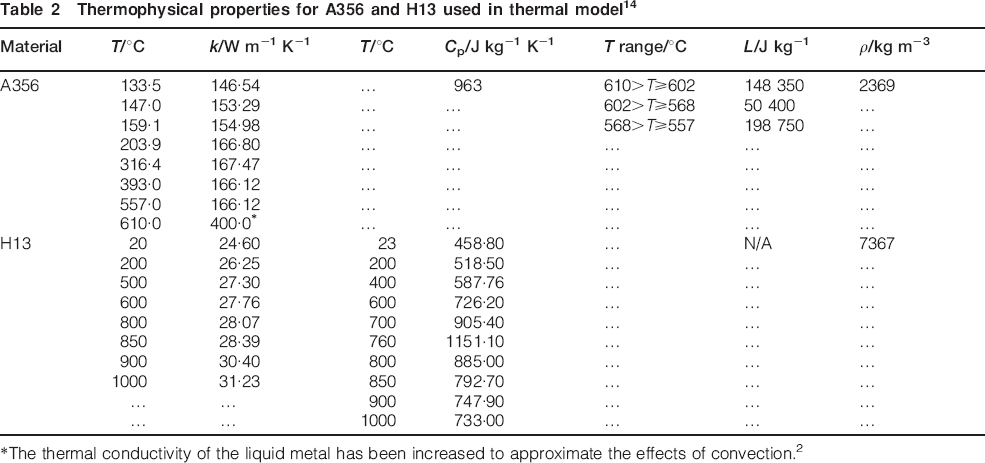
*The thermal conductivity of the liquid metal has been increased to approximate the effects of convection.2

Initial conditions

The effects of filling on the initial temperature of the casting and die have been neglected in the model based on previous process measurements which showed the little temperature change during filling. Therefore, the casting is initialised at a uniform temperature of 690°C at the start of each cycle. In the die, a uniform initial temperature of 400–440°C (specified based on the measured initial die temperature) is assumed for the first cycle and in subsequent cycles, the temperature distribution at the end of the previous cycle is used as the initial temperature.

Boundary conditions

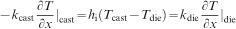
A variety of boundary conditions are needed to properly describe the flow of heat from the casting to the die and then to the surrounding environment. Moving outward from the casting, the first boundary condition encountered is at the interface between the casting and the die. The heat flux at this interface is controlled by the interfacial thermal resistance and is defined as (2) where h_i is the interfacial heat transfer coefficient (W m⁻² °C⁻¹). Based on surface orientation (i.e. horizontal, vertical or angled), the casting/die interface was partitioned into eight sections marked as S1–S8 in Fig. 1. For each section, maximum and minimum values of the interfacial heat transfer coefficient were defined along with a temperature range over which a linear transition occurs. A trial and error procedure was employed to determine the initial contact heat transfer coefficient (h_max = 4000 W m⁻² °C⁻¹) and the subsequent reduction in interfacial thermal resistance due to solidification shrinkage (h_min = 400–1200 W m⁻² °C⁻¹) for each section. The minimum interfacial heat transfer coefficient was increased on those sections that were expected to maintain improved contact because of the effects of gravity. Table 3 summarises the heat transfer coefficients and temperature ranges over which the heat transfer coefficient was ramped from h_max to h_min for the eight interface sections.

Table 3

Heat transfer coefficients and linear ramp temperature range applied along casting/die interface sections

Interface section	T range/°C	h_min/W m⁻² K⁻¹	h_max/W m⁻² K⁻¹
1 (trial 3)	540–560	400	4000
1 (trial 4)	565–585	400	4000
1 (trial 6)	540–560	400	4000
2	564–584	1200	4000
3	568–588	1200	4000
4	540–560	1200	4000
5	567–587	400	4000
6	540–560	1200	4000
7	540–560	1200	4000
8	540–560	1200	4000

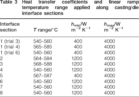
The heat transfer conditions summarised in Table 3 were rationalised by considering the effects of gravity, casting shrinkage and casting surface orientation. The finish and topology of the casting surfaces were also considered in regards to the data in Table 3. For example, h_min for interface sections 1 and 5 were assigned the smallest because their orientations were such that casting contraction and gravity effects combined to produce significant gaps. Higher temperature ranges, over which the heat transfer coefficients were ramped, were selected for sections 2 and 3 versus sections 6 and 7. This definition is consistent with the heat transfer decreasing earlier (i.e. with higher temperatures) higher up in the die because reduced effects of weight of the casting. Finally, sections where the casting was expected to rest on or to bulge out toward and maintain contact (sections 2–4 and 6–8) were defined with a high minimum heat transfer coefficient (1200 W m⁻² °C⁻¹).

To account for the additional heat supplied by the liquid metal contained in the riser tube, a temperature constraint was set on the surface representing the inlet from the sprue. In the process the casting remains in contact with this liquid metal after the die is filled and the die remains attached to the holding furnace. Therefore, the temperature constraint was defined as a function of time, starting at the initial casting temperature (i.e. 690°C) and decreasing linearly between 3 s (0 s is the time when the filling process is complete) and 37 s (when the furnace pressure is released) to 600°C during the casting cycle. The temperature decrease and the time over which this occurs were based on the trends observed in the temperature measurements.

Although the flow of liquid metal and its effects on heat transfer to the die during filling are not included in the model, the heat transfer along the casting/die interface was initiated as a function of filling time to link the heat transfer to the die to the filling event. Metal height was assumed to vary linearly during filling based on the linear pressure ramp applied during plant trials. Therefore, the heat transfer across the casting/die interface was activated as a linear function of time based on the calculated metal height.

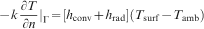
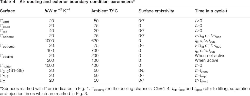
Continuing outward from the casting, boundary conditions were defined on the surfaces defining the internal cooling channels to include the effects of forced air convective cooling. Heat transfer coefficients and cooling air temperatures were defined based on temperature measurements and trial and error fitting. On the exterior surface of the die, the boundary condition used to describe the heat transfer to the ambient environment surrounding the die, including both convective and radiative effects, has the form (3) where n is the outward pointing direction normal to the surface Γ, h_conv is the convective heat transfer coefficient, h_rad is the equivalent radiative heat transfer coefficient, T_surf is the surface temperature and T_amb is the ambient environment temperature. The equivalent radiative heat transfer coefficient is calculated using (4) where σ is the Stefan–Boltzmann constant (5·669×10⁻⁸ W m⁻² K⁻⁴) and ϵ is the emissivity of the surface. The parameters of the forced air cooling and exterior boundary conditions are summarised in Table 4.

Table 4

Air cooling and exterior boundary condition parameters*

Surface	h/W m⁻² K⁻¹	Ambient T/°C	Surface emissivity	Time in a cycle t
Γ_side	20	50	0·7	t>0
Γ_back	20	75	0	t>0
Γ_top	40	20	0·7	t>0
Γ_bottom1	20	75	0·7	t<t_fill or t>t_sep
Γ_bottom1	1000	620	0	t_fill⩽t⩽t_sep
Γ_bottom2	20	75	0·7	t<t_fill or t>t_sep
Γ_bottom2	100	700	0	t_fill⩽t⩽t_sep
Γ_cooling	20	200	0	When not active
Γ_cooling	200	100	0	When active
Γ_holder	1000	400	0	t>0
Γ_D–C(S1–S8)	20	50	0·5	t>t_eject
Γ_D–S	20	50	0·7	t>t_sep
Γ_C	20	50	0·7	t>t_eject

*Surfaces marked with Γ are indicated in Fig. 1. Γ_cooling are the cooling channels, Ch#1–4. t_fill, t_sep and t_eject refer to filling, separation and ejection times which are marked in Fig. 3.

Solution procedure

Within ABAQUS, the mathematical model predicts the evolution of the casting and die temperature distribution for a single casting cycle. A perl language based wrapper script was written to automate the model allowing it to run continuously like an operating casting process. The wrapper communicates with and controls the model in a manner similar to an industrial controller and a casting machine. Operating in this manner, the process model acts as a virtual process which runs continuously and can be programmed with varying input conditions.

The predicted casting temperatures are used to calculate if/when liquid encapsulation occurs in each casting cycle and the volume of liquid that is encapsulated. A post-processing programme was developed to determine when a portion of the casting is isolated from the liquid metal supply of the sprue. This involves performing a search to identify all of the nodes in the domain, with temperatures higher than a critical temperature for feeding, which are not connected to the sprue by a path of interconnected nodes. The critical temperature for feeding was assumed to be 568°C based on a critical fraction solid of 0·8.14 The nodes identified in this manner represent a pocket of encapsulated liquid metal which has the potential to form macroporosity as the isolated liquid metal solidifies. Example predictions of liquid encapsulation are presented in Fig. 2. In Fig. 2, the dark (red) regions represent metal with temperatures greater than the critical temperature and the blue regions are at temperatures below the critical temperature. The sequence of liquid metal encapsulated evolves during a casting cycle and may (or may not) include: the encapsulation of a volume of liquid in the upper section (refer to Fig. 2a); and as solidification proceeds, encapsulation may occur in the lower section (refer to Fig. 2b). The total volume of encapsulated liquid is the addition of these two volumes. The volume of encapsulated liquid for each region as well as the total is calculated for use as an indicator of the potential extent of macroporosity.

Figure 2

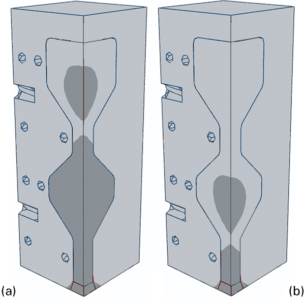
Predicted liquid encapsulation evolution in a upper and b lower section

Model validation

To provide the data necessary to fit the boundary conditions of the model and validate the temperature predictions, a plant trial was conducted at NRC CANMET-MTL's LPDC facility, located in Ottawa, Canada. The LPDC machine at this facility was adapted for casting light metals and its operation is atypical in that the die lifts off the holding furnace each cycle and rotates to the side before ejection. A casting cycle begins when the die closes and rotates, placing it in contact with the holding furnace. Metal is forced up a joint pipe and into a sprue to fill the die when the air above the liquid metal in the holding furnace is pressurised. The casting solidifies as heat is transferred to the die. Four forced air or water cooling channels in the die are used to cool the die. Air or water coolants are options depending on desired cooling rates to produce different impacts on the die temperature. After a predetermined time, the pressure in the holding furnace is released and the die is then rotated away from the holding furnace. The die is opened and the casting is removed manually. Before the start of the next cycle, the die remains open and cools.

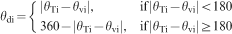
A schematic plot of the die temperature variation during a casting cycle and the related process timing parameters are shown in Fig. 3. The die temperature exhibits a characteristic variation with time during each casting cycle. Initially, the die temperature decreases before the liquid metal filling the cavity at t_fill. The temperature increases rapidly after filling as a large amount of heat transfers from the casting to the die. As the die temperature increases and the casting solidifies, the heat flux to the die decreases and the temperature in the die plateaus. When the die rotates away from the holding furnace t_sep, the temperature decreases as the casting continues to cool and solidify. Finally, the cooling rate in the die increases when casting is ejected (t_eject) and the temperature continues to decrease until the end of the cycle.

Figure 3

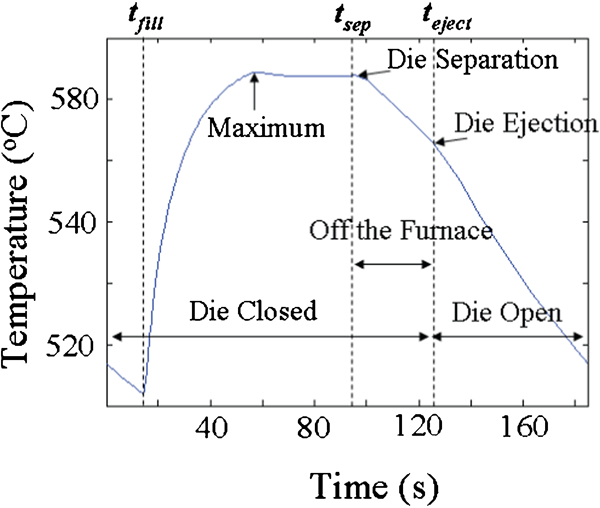
Single cycle die temperature variation

Low pressure die casting trials

The plant trials conducted for this investigation used a die based on the geometry shown in Fig. 1. A series of 12 casting trials were conducted in open loop mode with cycle timing performed manually. Each casting trial condition was run until cyclic steady state, where the die temperatures at the start and end of the casting cycle are within 1°C, was achieved (a minimum of 10 shots). When planning the plant trial, a start and end temperature difference of 0·1°C was targeted to define steady state operation. However, in practice, the timing for each stage of the casting cycle was performed manually and process disturbances occurred regularly during each trial which made it impractical to determine when cyclic steady state occurred to within this tolerance. From the 12 trials, three representative trial conditions, summarised in Table 5, were selected for use in this investigation to examine the effects of die closed time, die open time and cooling duration (only cooling channel 1 was active).

Table 5

Experimental process parameters

Trial no.	Die closed time/s		Die open time/s	Cooling channel 1		Shots no.
Trial no.	Pressure* on	Pressure off	Die open time/s	Time/s	Flowrate/L min⁻¹	Shots no.
3	30	90	45	…	…	20
4	30	90	60	…	…	13
6	30	90	45	120	600	15

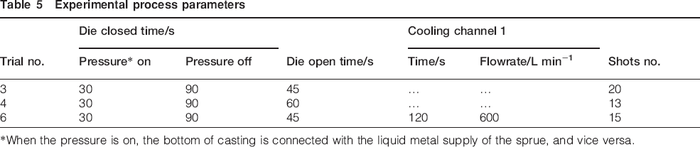
*When the pressure is on, the bottom of casting is connected with the liquid metal supply of the sprue, and vice versa.

The die temperatures were measured at eight locations in the die (as indicated in Fig. 1) via type E thermocouples mounted 5 mm below the die surface. Temperature data were collected with a sampling rate of 1 Hz from the start of casting until cyclic steady state was achieved.

Results

The predicted (red lines) and measured (blue symbols) die temperatures at three of the eight thermocouple locations are compared in Fig. 4 for representative steady state casting cycles from casting trials 3, 4 and 6 (refer to Table 5 for details of process parameters). Within the results for each trial condition, the temperatures measured at the three locations show consistent trends. The temperature at TC#2 is the lowest among the three thermocouple locations reported, because this location is both closest to the exterior mounting surface of the die where heat is lost to the casting machine and closest to the cooling channel activated in trial 6. Conversely, the highest temperatures were measured by TC#5 because it is furthest from the external surface of the die and in a location surrounded by a considerable thermal mass. Considering the effect of operational conditions for a given die location, the subplots in Fig. 4 indicate that increased die open time (trial 4) and the activation of forced air cooling (trial 6) result in decreased die temperatures. The largest decrease in die temperature and the most localised effect, was measured at TC#2 when forced air cooling activated because this location is nearest to the active cooling channel.

Figure 4

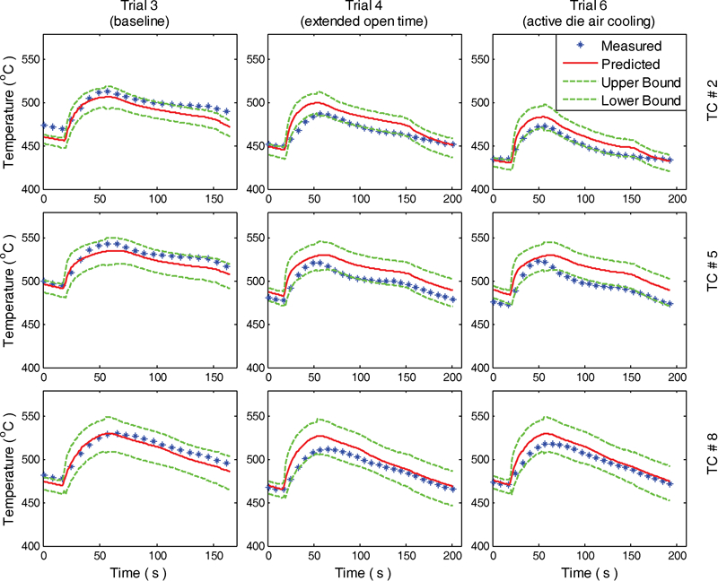
Comparison plot of predicted and measured data with consideration of uncertain factors

Despite attempts to alter the boundary conditions to improve the temperature predictions, differences still exist between the predicted (red line) and measured temperatures (blue symbols) presented in Fig. 4. The discrepancy between the predicted and measured data may be due to uncertainty and/or variability under the operational conditions achieved in the trial which have not been accounted for in the model. In an attempt to assess the sensitivity of the model predictions, an uncertainty analysis has been performed. After systematically varying the model input parameters, potential errors contributing to discrepancy between the predicted and measured temperatures are:

random errors

μ₁: the error from varying forced air cooling heat transfer coefficient (h = 10–20 W m⁻² °C⁻¹)

μ₂: the error from varying thermocouple positions (uncertainty in each direction ±2 mm)

μ₃: the error from varying linking time between casting and die during the process where casting was separating from die in a cycle

systematic error

μ₄: the error from cycle timing uncertainty (±2 s).

Following a statistical approach to estimate the propagation of uncertainty in this system,15 the combined error due to uncertainty in the identified parameters can be calculated as the root mean square of the three independent random error factors, expressed as follows (5) where μ₂ is defined as the root mean square of μ₂ along x, y and z directions. Based on the composite errors of both the random and systematic errors,15 the upper [T(t)⁺] and lower [T(t)⁻] bounds of the model predictions are expressed as follows (6) where T(t)_pred is the die temperature predictd by the model, and are the positive and negative effects of μ_i on the die temperature, as a function of time t, respectively.

The sensitivity of the temperature predictions to the identified uncertainty factors was calculated with equation (6). The lower and upper bounds of the temperature predictions are plotted in the Fig. 4 as green dashed lines. For the most part, the measured temperatures fall within the temperature range defined by these curves indicating that identified uncertainty factors may explain the differences between the predicted and measured temperature data. Based on this analysis and the comparison between the predicted and measured temperatures, the model is assumed to adequately describe the casting process enabling its use in further analysis.

Determining optimal measurement location

The virtual process, operating continuously, has been used to simulate an industrial casting operation. This framework allows process parameters to be changed and their effects to be evaluated as in a plant trial. Using the virtual process, predicted die temperatures were analysed to determine their correlation with the predicted volume of encapsulated liquid. Assessing the correlation throughout the die allows the determination of the optimal location to measure die temperature for correlation with the volume of ecapsulated liquid.

Process operational parameters

Three control variables in the casting process were expected to affect the amount of macroporosity: die closed time, die open time and cooling duration. The most commonly used technique to assess the contribution of control variables is the trial and error method.11 However, the Taguchi method, an experimental optimisation method, is more rigorous and has been widely used in other applications.16^–18 In the current study, it was applied to the virtual process to investigate the influence of control variables on the formation of macroporosity represented by the volume of encapsulated liquid. An orthogonal array was used to systematically vary and test the different levels for each of the control variables. The results indicated that two variables greatly affect the magnitude of the encapsulated liquid volume: die closed time and cooling duration (when water cooling is considered). Hence, these two variables were considered as control inputs and the remaining discussion and analysis presented in this study will be limited to these variables.

Method of analysis

The virtual process was run for a range of process operational conditions to provide data suitable for correlating die temperatures with the volume of encapsulated liquid. The process inputs of die closed time and cooling duration were varied from 105 to 205 s in increments of 5 s and from 0 to 24 s in 3 s increments respectively while the die open time was fixed at 60 s. The combination of these parameters represents 189 (21×9) operational conditions. For each condition, the virtual process was run until the cyclic steady state was achieved. For this portion of the study, cyclic steady state was defined as less than a 0·01°C difference between the cyclic start and finish temperatures throughout the die.

From the cyclic steady state result of each process condition, the volume of encapsulated liquid was calculated and the die temperature versus cycle time at each thermocouple location was extracted in a post-processing operation. The die temperature data were further processed to extract the temperature at two times during the casting cycle, the maximum die temperature and the die temperature at ejection (refer to Fig. 3), at each thermocouple location for correlation with the volume of encapsulated liquid. These temperatures were selected for evaluation because they represent characteristic points in the casting cycle that are easy to identify. The extracted data were used to construct response surface plots for the candidate temperatures and the volume of encapsulated liquid.

In Fig. 5, the response surfaces of the volume of encapsulated liquid and the maximum die temperature are overlaid for the upper and lower die locations (TC#2 and 8 in Fig. 1). The response surface of the volume of encapsulated liquid, which is location independent, is minimised when the die closed time is 190 s and the cooling duration is 0 s, i.e. no water cooling. Although this optimal point suggests that water cooling is detrimental in that it increases the volume of encapsulated liquid, a compromise would likely be necessary to increase the production rate by reducing the die closed time. The maximum die temperature at both thermocouple locations generally increases with decreasing cooling duration. The response surfaces of the maximum die temperature and the volume of encapsulated liquid show a good correlation for the combination of longer cooling duration and longer die closed time at the lower die location (TC#8). However, the response surface of maximum die temperature at the upper die location (TC#2) exhibits less curvature. Therefore, there is only a small region (along the diagonal defined by the minimum volume of encapsulated liquid versus die closed time) of good correlation at the upper die location. Correlation here is executed between the gradient of the maximum die temperature and negative gradient of the volume of encapsulated liquid, where the gradient of a scalar field at one point is mathematically defined as the direction in which the parameter rises most quickly. A good correlation of these two parameters indicates that the direction to increase the maximum die temperature is just the direction to decrease the volume of encapsulated liquid.

Figure 5

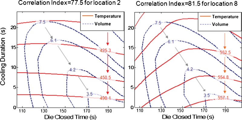
Contours of maximum die temperature and volume of encapsulated liquid for die locations corresponding to TC#2 and 8

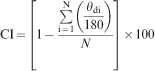
A metric to quantify the correlation of the response surfaces of the volume of encapsulated liquid and the die temperature has been developed. A ‘correlation index’ (CI) is computed based on the differences in the local normal of the two response surfaces over the process input space according to where θ_di is the angular difference of θ_vi and θ_Ti, θ_di ∈ [0, 180] and N is the number of operational conditions. θ_vi is the angle of negative gradient of the volume of encapsulated liquid response surface at the ith operational condition and θ_Ti is the angle of gradient of the die temperature response surface at the ith point, θ_vi and θ_Ti ∈ [0, 360]. Specifically, θ_di is computed as follows The quantities calculated are shown graphically in Fig. 6. When the response surfaces are identical, the CI hence equals 100 where there are no differences between the gradient of the maximum die temperature and the negative gradient of volume. The rationale for this metric is that if the response surfaces are similar (i.e. CI approaching 100), the rising variation of die temperature at this location can be directly related to the decreasing variation of the volume of encapsulated liquid.

Figure 6

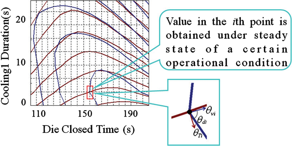
Schematic plot of CI for region

The CI calculated at a given location in the die represents the average correlation over the operational range considered. The standard deviation of CI at a given location can also be calculated for use as a measure of the variability of correlation over the operational range. The standard deviation of the correlation at a die location is computed as follows where μ is the mean of θ_di.

Expanding the application of this technique, the CI and its standard deviation were calculated at all locations in the die. The die location with the highest CI between the die temperature and encapsulated liquid volume and the smallest standard devaition represents the optimal location within a die to monitor temperature for the purposes of relating it to macroporosity. To accomplish this, the post-processing operation to calculate the volume of encapsulated liquid and extract the die temperature data was considered at each node in the die geometry. The resulting data set was then used to calculate the CI and standard deviations using Matlab.

Results and discussion

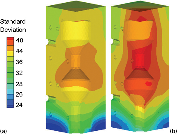
The contour plots of the CI calculated with the two candidate die temperatures: maximum die temperature and die temperature at ejection are shown in Fig. 7. In Fig. 7, the entire casting volume was considered when determining the liquid encapsulation. The maximum die temperature CI is the highest (84·25) at the bottom of the die, near the metal inlet on the casting/die interface, close to the parting line. The CI decreases with the increasing distance from this location and reaches its lowest value (77·00) at the top of the die. The CI calculated for the die temperature at ejection exhibits a similar variation albeit shifted to lower values (CI ranging from 70 to 82). Additionally, there is a region of low CI present on the casting/die interface in the lower enlarged section of the die. For both candidate die temperatures, the hightest values of CI are observed at the bottom of the die, near to the casting inlet.

Figure 7

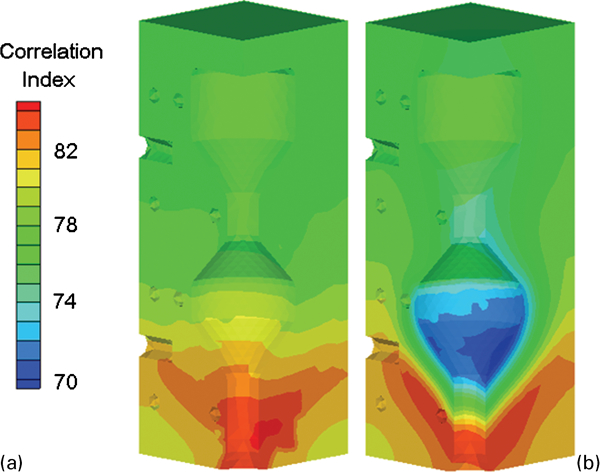
Contour plots of CI based on two candidate temperatures: a maximum die temperature and b die temperature at ejection with total volume of encapsulated liquid (refer to Fig. 2)

Table 6 summarises the CI values at the eight locations where thermocouples were installed. The data indicate that the CI for the maximum die temperature is higher than that for the die temperature at ejection for all locations except at the TC#8 location. The maximum die temperature CI shows a trend of gradual increase from locations 1 to 8, whereas the CI for the die temperature at ejection does not show a consistent trend. Consistent with the contour plot, Table 6 suggests that the best location to monitor temperature for correlation with the volume of encapsulated liquid is TC#8 near the bottom of the die.

Table 6

Correlation index calculated at TC locations

TC#	CI
TC#	Maximum die temperature	Temperature at ejection
1	77·20	75·95
2	77·50	77·14
3	77·78	76·42
4	77·78	75·41
5	78·24	76·86
6	79·91	75·25
7	81·38	74·34
8	81·50	83·84

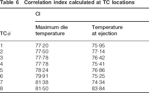
Figure 8 shows the contour plots of the standard deviation of CI for the two candidate die temperatures. The bottom of the die has the smallest standard deviation of CI for both temperatures, which means that the CI in this area has the smallest dispersion over the operational range considered. In other words, the CI at the bottom of the die is the least sensitive area to variability in the operational conditions. Therefore, the bottom of the die near the casting/die interface exhibits both the highest CI and the smallest standard deviation, indicating that this is the best location to monitor temperature for correlation to liquid encapsulation within the entire volume of the casting. Considering the casting geometry, this result is expected since this location is near the metal inlet which is the critical location for liquid encapsulation in the entire casting volume. However, the methodology and metric employed in this study enable a quantitative determination of this location.

Figure 8

Contour plots of standard deviation for CI based on two candidate temperatures: a maximum die temperature and b die temperature at ejection with total volume of encapsulated liquid (refer to Fig. 2)

The CI analysis was performed on a subsection of the casting volume to determine what effect if any region of interest had on the results. Figure 9 shows a contour plot of CI for the two die temperatures where the volume of encapsulated liquid was evaluated in the upper (enlarged cross-section) volume of the casting. In this case, the region of the highest CI values has moved up toward, but remains below the narrow cross-section zone in the middle of the die. The reason may lie in that the temperature variation for the area below narrow cross-section zone has the stronger chronic effect on the formation of the upper volume of encapsulated liquid, hence causing the highest CI (computed under steady state) for this area. The standard deviation of the CI's based on liquid encapsulation in the upper volume (Fig. 10) indicates that the largest variation in CI is expected in the narrow cross-section zone. Therefore, the CI in this region will be more sensitive to changes in operational conditions involved, making the correlation of die temperature to volume of encapsulated inaccurate.

Figure 9

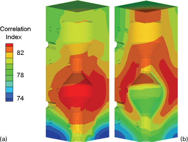
Contour plots of CI based on two candidates for die temperatures: a maximum die temperature and b temperature at ejection with upper volume of encapsulated liquid (refer to Fig. 2a)

Figure 10

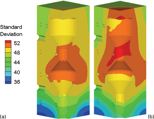
Contour plots of standard deviation for CI based on two candidates for die temperatures: a maximum die temperature and b temperature at ejection with upper volume of encapsulated liquid (refer to Fig. 2a)

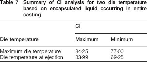
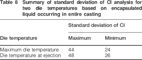
Tables 7 and 8 summarise the CI and standard deviation results for the two candidate die temperatures: the maximum die temperature and the die temperature at ejection, based on the encapsulated liquid occurring in the entire casting volume. The maximum die temperature shows higher overall CI values and smaller standard deviation of CI, and therefore is a better indicator of the volume of encapsulated liquid. This indicates that the maximum die temperature is a better correlation to the volume of encapsulated liquid and exhibits the least amount of variability with changes in operational conditions. When considering liquid encapsulation in the upper volume only, there is little difference between difference from the die temperature at ejection for both the CI and the standard deviation. Based on the first set of results, the maximum die temperature is proposed as an indicator for the volume of macroporosity occurring in the casting.

Table 7

Summary of CI analysis for two die temperature based on encapsulated liquid occurring in entire casting

Die temperature	CI
Die temperature	Maximum	Minimum
Maximum die temperature	84·25	77·00
Die temperature at ejection	83·99	69·25

Table 8

Summary of standard deviation of CI analysis for two die temperatures based on encapsulated liquid occurring in entire casting

Die temperature	Standard deviation of CI
Die temperature	Maximum	Minimum
Maximum die temperature	44	24
Die temperature at ejection	48	26

Conclusions

A methodology has been developed to analyse the correlation between the die temperature and the volume of encapsulated liquid in a casting with the intent of providing a means of assessing macroporosity formation based on a process measurement. To test the methodology, a mathematical model of an experimental casting process capable of predicting the temperature distribution in the die and casting as well as the volume of encapsulated liquid was developed. The model was shown to be accurate within a range of uncertainty attributed to various parameters by comparison to thermocouple data from a plant trial. The model was used to assess the suitability of different in-cycle die temperatures and based on these to determine the optimal location to monitor temperature in order to minimise liquid encapsulation. Overall, by identifying die locations whose temperatures are closely correlated with casting defects, this methodology will aid in the development of an advanced control methodology to minimise defect formation.

References

Bonollo

, Urban

, Bonatto

, Botter

: ‘Gravity and low pressure die casting of aluminium alloys: a technical and economical benchmark’, Metall. Ital. , 2005, 6, 23–32.

Zhang

, Maijer

, Cockcroft

: ‘Development of a 3-D thermal model of the low-pressure die-cast (LPDC) process of A356 aluminum alloy wheels’, Mater. Sci. Eng. A , 2007, A465, 295.

Andresen

: ‘Die casting engineering’; 2005, New York, Marcel Dekker.

Esdaile

, Nguyen

, de Looze

, Murray

: Proc. 1st Int. Non-Ferrous Processing and Technology Conf., 213–218; 1997, Warrendale, PA, USA, TMS International.

Muller

, Feikus

: AFS Trans. , 1996, 104, 1111–1117.

Singh

, Mallinson

, Panton

, Palle

: ‘Die design strategy for improved productivity and quality in die casting’, AFS Trans. , 1999, 99, (25), 127–128.

Wilkinson

, Wilson

, Connor

, Smith

: ‘CIM and control of pressure die-casting in the automotive industry’, Comput. Control Eng. J. , 1994, 5, (3), 125–130.

Palanisamy

, Nagarajah

, Graves

, Iovenitti

: ‘A hybrid signal pre-processing approach in processing ultrasonic signals with noise’, Int. J. Adv. Manuf. Technol. , 2009, 42, (7–8), 766–771.

Cox

, Harding

: ‘Influence of tilt filling on Weibull Modulus of 2L99 aluminium investment castings’, Mater. Sci. Technol. , 2007, 23, (2), 214–224.

10.

Jeffery

: ‘Non-destructive testing: 5 ways to ensure defect-free deliveries’, Modern Cast. , 88, 1998, 49–52.

11.

Bishenden

, Bhola

: ‘Die temperature control’, Proc. 20th Int. Die Casting Cong. and Exposition, Cleveland, OH, USA, November 1999, North American Die Casting Association, 161–164.

12.

Thompson

, Cockcroft

, Wells

: ‘Advanced light metals casting development: solidification of aluminium alloy A356’, Mater. Sci. Technol. , 2004, 20, 194–200.

13.

American Society for Metals: ‘ASM metals reference’, 2nd edn; 1984, Metals Park, OH, ASM.

14.

Mills

: ‘Recommended values of thermophysical properties for selected commercial alloys’; 2002, Cambridge, Woodhead Publishing.

15.

Drosg

: ‘Dealing with uncertainties: a guide to error analysis’, 2nd edn; 2009, Berlin, Springer.

16.

, Chang

: ‘Use of Taguchi method to develop a robust design for the magnesium alloy die casting process, Mater. Sci. Eng. , 2004, 379, 366–371.

17.

Kackar

: ‘Off-line quality control, parameter design and the Taguchi method’, J. Qual. Technol. , 1985, 17, (4), 176–188.

18.

Logothetis

: ‘The role of data transformation in the Taguchi analysis’, Qual. Reliab. Eng. Int. , 1988, 4, 49–61.