






Abstract
The present paper provides a comprehensive approach to the use of simulations to determine sampling errors for three broad classifications of analyte characteristics: low concentrations of analyte mostly occluded within gangue grains, low concentrations of analyte occurring mainly as liberated grains and higher analyte concentrations. Poisson distributions are used for simulations for the first two of these classifications and a binomial distribution is used for the third. The methodology requires that samples are screened and each size fraction is weighed and assayed. Fortran computer codes and accompanying data sets are provided for each of the three classifications in the accompanying Appendixes. Outputs from the simulations are compared with the error variances generated by Gy's sampling formula.
Introduction
Previous attempts at dealing with this problem (Royle, 2002) used a Poisson distribution for the simulations. While this methodology is entirely appropriate for low concentrate analytes, it leads to high variances when higher analyte concentrations are present. Simply, a Poisson distribution is suitable for low concentration analytes whereas a binomial distribution, following Gy's approach (Gy, 1998), appears to be more suitable for higher concentrations.
The purpose of the present paper is to present a complete approach to the use of simulations to determine sampling errors. In doing so, it is useful to approach the problem using three broad classifications of analyte characteristics: low concentrations of analyte mostly occluded within gangue grains, low concentrations of analyte occurring mainly as liberated grains and higher analyte concentrations. Three computer programs are provided which produce the distributions and statistics of samples drawn from lots of granular material for each of these classifications.
As Gy's sampling formula will be used to check the outputs of the simulations it is useful to begin with a summary of the formula and the associated parameters.
Gy's sampling formula
Gy's sampling formula (Gy, 1979, 1998) is a practical tool, which, used intelligently, serves as a useful guide to good sampling practice. In its most common form, it expresses the variance of the sampling error as


L is the liberation size for mineral particles, i.e. the maximum particle diameter that ensures complete liberation of the mineral from the gangue. L is measured in cm. m is the mineralogical composition factor, which is calculated from

For gold, the mineralogical composition factor is calculated as


When ML is large, equation (1) reduces to

The major problem in using Gy's formula in practical applications is in determining the liberation factor.
Poisson, binomial, normal distributions and possible biases
These three distributions and their approximations are used in the simulations, so they must be examined to see what biases they may create and how serious their effects may be.
A Poisson distribution models the frequencies of occurrence of infrequent events. Nuggety analyte grains, in samples of the weights taken in practice, occur infrequently and so appear to be suitable for treatment by a Poisson distribution (Gy, 1979; Venter, 1982; Royle, 2002). Such grains are the cause of the highest sampling errors.
A computational problem may arise when high grain counts occur because of a limit set on the maximum number handled by the exponentiation function. However, when the grain count N is large the Poisson distribution approximates a normal distribution with mean N and variance N. Accordingly a change was made from a Poisson to a normal distribution beyond grain counts of 500. The data in Table 1 were generated to test the convergence between the two distributions.
Testing goodness of fit when Poisson distribution is modelled by normal distribution (Poisson parameters are N = 500, variance = 500; corresponding normal distribution has same parameters)

Table 1 compares the corresponding frequencies in the two distributions. Overall the fit is good and there is no global bias, but at low grain counts the normal distribution is negatively biased with respect to the Poisson, and positively so at high grain counts, the bias reducing to zero at the mean.
As grain counts less than 500 will be processed by the Poisson distribution this leaves only those above 500 to be processed by the normal approximation, which at first sight will retain a small positive bias in the computed values of assay outcomes and variances. There is no discernible evidence of this happening in the examples given later. Differences between actual and computed assays are no greater than what may be expected from Monte Carlo simulations.
One reason for the apparent absence of bias is that as grain counts increase the sampling error diminishes. The total sampling error is the sum of the errors from the individual fractions. Errors from fractions with high grain counts make only small contributions to the total error, reducing the effect of small differences between the values calculated by a Poisson and a normalised distribution. Also, assays in the tails of the normalised distribution occur with decreasing frequencies, which further mitigates the effects of their biases.
Gy (1979) used a binomial distribution in his seminal work on sampling. It has the advantage of flexibility, as in appropriate circumstances it can be approximated either by a Poisson or by a normal distribution. Higher concentrations of analyte, and hence higher grain counts, make the Poisson distribution an unsuitable choice in such circumstances. Following Gy's lead, a binomial distribution will be tried.
For the same reasons given earlier the change from a binomial to a normal distribution will be made at grain counts above 500. Table 2 shows the results of modelling a binomial with a normal distribution when, using the usual binomial notation, N is set to 500 and P to 0·65. (P = 0·65 is a typical value found in the iron data used later.)
Testing goodness of fit when binomial distribution is modelled by normal distribution (binomial parameters are N = 500, P = 0·65; corresponding normal distribution has parameters: mean = 325, variance = 113·75)

Overall, the fit is good with no global bias, but at low grain counts the normalised distribution is negatively biased with respect to the binomial, and positively so at higher grain counts. The biases are somewhat larger than those found in Table 1 from the Poisson distribution.
Some typical iron ore data were examined, taking sample weights of 1, 10 and 100 kg. Taking 1 kg samples ensured that more of the estimates of the size fractions’ means and errors would be simulated by the binomial distribution, 100 kg samples mostly by the normalised distribution, and 10 kg samples occupying a mid-way position (see Table 3).
Means and errors from 1, 10 and 100 kg samples using binomial and normalised distributions
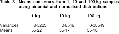
The variances of the 1 kg samples were 10 times those of the corresponding 10 kg samples and 100 times those of the 100 kg samples, as demanded by sampling theory. The simulated means coincide well enough. Thus, although there are differences between the tails of the binomial and its normalised distribution, values in the tails are generated less frequently and so have a relatively small effect on the ultimate outcomes. Accordingly, the binomial distribution was chosen for simulations of materials with higher analyte content.
Sampling errors for low concentrations of analyte
This section covers the two low concentration classifications and applies to mixtures of solids whose assays, made on samples of weights used in normal practice, may be characterised by Poisson distributions. The first applies where solids have been crushed to an extent that leaves most of the analyte still occluded in the gangue grains, i.e. not liberated. The second applies where a substantial proportion of the analyte is liberated, e.g. after pulverising. It can be applied as well to alluvials and powder mixtures.
In the following examples, simulations have been used to determine sampling errors. They are probably useful, too, for answering ‘What if?’ questions, such as ‘How would the sampling error change if a certain selection stage was omitted?’ and ‘Do we need to examine this number of size fractions?’.
Program NONLIB.FOR deals with non-liberated particles of analyte, and LIB.FOR with liberated grains. Practical applications of the two are best illustrated by examples.
Non-liberated grains
In all likelihood the finer size fractions contain liberated analyte particles. It will be demonstrated that the input from these fractions to the total sampling error is insignificant.
Example no. 1
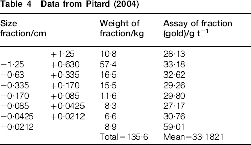
The data for this example are taken from Pitard (2004) and are reproduced in Table 4.
Data from Pitard (2004)
Simulation
The data were processed by program NONLIB.FOR, which requires the creation of a file such as PITARD.DAT, listed and explained as follows:
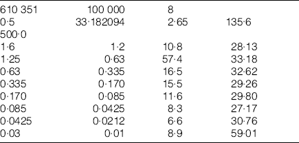
610 351 initial random number required by subroutine URAND to start generating random numbers. Any five-figure or longer number will do for this purpose.
100 000 number of simulations. 50 000 is a reasonable number.
8 number of size fractions.
0·5 shape factor, e.g. 1 for cubes, 0·5 for spheres.
33·1821 assay of the lot (g t−1), calculated from the weights and assays of the fractions.
2·65 specific gravity of the gangue.
135·6 weight of the lot (kg).
500·0 weight of the sample (g).
The last eight lines are taken from Table 4. The limits of the coarsest fraction have been set to 1·6 and 1·2 cm to give a mean diameter of 1·4 cm. Similarly, the limits of the finest fraction have been set to 0·03 and 0·01 cm to give a mean diameter of 0·02 cm. Note that all units are specified exactly, as is required by the program.
A listing of NONLIB.FOR is given in Appendix 1. Comment statements have been included to assist in understanding the operations of the program. In addition to producing the statistics of the sampling error, the program produces the sampling distribution and plots it if required.
Low grain counts in size fractions are assigned to Poisson distributions. Although a Poisson distribution with a mean as low as six is not statistically different from a normal distribution with a mean and variance of six (chi-square test), an examination of the frequencies within the corresponding groups shows that this assumption leads to slightly increased variances.
Appendix 2 shows how the Poisson and normal distributions converge as the grain counts are increased. In Bias C, the biases within the groups have been weighted by their relative frequencies to show that although the biases towards the tails of the distribution are greater than those around the mean, they occur less frequently and so their effect is diminished.
It was decided that a Poisson distribution would apply to grain counts below 400, and the assimilation of higher grain counts into normal distributions would incur no serious errors.
There are several variables in a size fraction:
the sizes of the gangue grains
the sizes of the analyte grains within them
the number of analyte grains within each gangue grain.
Taking each size fraction in turn, the program encapsulates the three variables into a single one. The analyte content of the fraction is assumed to be equally distributed between the gangue grains to produce ‘equivalent grains’, and it is the variation in the numbers of equivalent grains produced by random selections that gives rise to the variations in the simulated assays. For each simulation, each size fraction is simulated separately and the analyte from each is summed to give the final assay. Thus, for the Kth size fraction, FN(K) is the expected number of equivalent grains in the fraction. If there are fewer than 400, subroutine URAND generates a random number between 0 and 1. This number is checked against the table of cumulative Poisson probabilities and the number of grains so found, multiplied by W(K), gives the contribution made by that fraction to the total assay.
If FN(K) is greater than 400 it is treated as a normal distribution with mean and variance of FN(K), and standard deviation SD the square root of FN(K). URAND is entered 12 times to generate random multiples of the standard deviation consistent with a normal distribution.
SUM is the final assay, the sum of all the contributions from the individual fractions, and DIG is the difference between SUM and the assay calculated from the weighted sum of the fractions’ assays. DIG is used to calculate the remaining statistics.
The assays are allocated to 100 frequency groups, with M(IL) being the count of assays in the ILth group. These details finally appear as:
F the assay value at the end of the group
M(K) the count of assays in the group
FREQ(K) the relative frequency of M(K)
SUMF the cumulative relative frequency
These give the distribution of assay outcomes.
The rest of this part of the program determines and prints the statistics of the simulations. Subroutine PLOT may be called to give a graphical appreciation of the distribution; it can be useful to emphasise some point, e.g. results showing a markedly non-normal distribution.
The output from NONLIB.FOR and PITARD.DAT – PITARD.OUT – after removing zero frequency groups is shown in Appendix 3. If the program is run with a 50 g pulp, grain counts are 10 times smaller, the calculated assay is the same, and the variance is 10 times bigger.
NONLIB.FOR then examines the statistics of the individual fractions, calculating the contribution each makes to the whole pulp assay and to the whole pulp variance. This is performed for two reasons:
to check that the sums of the assays and the variances from the individual fractions agree with those of the whole pulp (apart from negligible divergences arising from simulations)
to view the error contribution from each fraction, possibly with a view to combining redundant fractions.
The sum of the fractions’ assays was 33·1922 g t−1, and of the fractions’ variances was 50·5395. The corresponding figures for the whole pulp are 33·1814 g t−1 and 50·7754, which are not significantly different to the values for the fractions.
The finer fractions have made only small additions to the total sampling variance. In this example the three fractions coarser than 3 mm (i.e. +0·335 cm in Table 4) comprise 62·5% by weight of the lot and contribute 99·7% to the total sampling error. The figures for the top two fractions are 50% of the weight and 97·2% of the variance.
Example no. 2
Data are taken from a gold-quartz deposit. Supervised by the author, a truck-load was screened into six size fractions. Each fraction was split into 16 subsamples on which duplicate assays were run, so each recorded assay is the mean of 32 assays. The data are given in Table 5.
Gold quartz deposit data

The quartz gangue had a specific gravity of 2·65. The rocks were roughly spherical and a shape factor of 0·5 was assumed. The largest were some 10 cm in diameter and a minimum diameter of 0·1 cm was assigned to the smallest. Accordingly, the following file, EXAMPLE2.DAT was set up for treatment by NONLIB.FOR, taking a 50 kg sample.
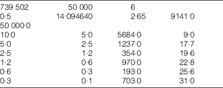
EXAMPLE2.OUT (Appendix 4) lists the output, which for the whole pulp gave an assay of 14·0895 and a variance of 8·8906. The individual fractions gave figures of 14·0986 and 8·8220.
Liberated grains
Program LIB.FOR, listed in Appendix 5, is used. N.B. ASSFRAC is now the contribution made by a fraction to the assay. ASSAY is thus the sum of the ASSFRACs.
The analyte content of each size fraction WG is determined in terms of mg. Next, the weight W (mg) of an analyte grain having a diameter of the average of the upper and lower size bounds is found. Thus, the ‘equivalent analyte grains’ are now composed of the analyte itself and they number FN ( = WG/W). The variations in the simulated grain numbers are expressed as sampling variances.
LIB.FOR is suitable for pulverised material where free grains form the majority. Now, the shape factor is of critical importance. With malleable minerals the horizontal axis disc pulveriser can produce an abundance of cylindrical or spherical particles. These are solid objects, with rock particles pressed into their surfaces.
Ring mills and single puck pulverisers tend to produce flakes, many of them appearing as ‘egg cartons’ in that rock particles are pressed into analyte cartons. During the initial stages of pulverising, malleable analyte grains are liberated and appear as large flakes, which further action by the mill then rolls into foliated cylinders. Continued pulverising splits these longitudinally into elongated flakes, which in turn are reduced further.
Thus, the plan area of a carton, as measured by the screen that retains it, may be different from the surface area of the unrolled carton and this will affect the calculated weight of such a grain. And mineral particles, because of adhering rock grains, are retained on screens through which the mineral particles alone could easily pass. This is certainly the case after screen fractions have been washed with HF. Hence, a microscopic examination of the pulverised product is essential and one makes the best estimate one can of the shape factor.
Example no. 3
This example uses data from Venter (1982) and Royle (2002). Pulverised brass particles were screened and two size fractions were selected, one ranging from 38 to 53 μm, and the other from 7·2 to 10·6 μm. The coarse fraction seemed to consist of spherical grains, and the fine fraction of flakes probably spalled off irregular grains as they were ground into spheres. As coarse grains would be the major contributors to the sampling error, a shape factor of 0·5 was used. A specific gravity of 8·8 was assigned to brass. A pulp was made up containing the equivalent of 5 g t−1 of the coarse fraction and 45 g t−1 of the finer, a total of 50 g t−1.
Two sample weights are used: 1 and 0·05 g. The values of the parameters in the data file BRASS.DAT, for the sample weight of 1 g, are:

The output from 1 g samples is listed under BRASS1.OUT in Appendix 6. In general there is good agreement between the whole pulp and the fractional statistics.
The second run using a sample weight of 0·05 g t−1 gave the results listed as BRASS2.OUT in Appendix 7. The grain counts showed that the coarse fraction had been treated as a Poisson distribution, the fine fraction as a normal distribution. The bimodality of the lot's constituents shows up clearly on the plot of the relative frequencies. A bimodal plot is not, of course, the target of one's endeavours if confidence limits are to have any meaning. The plot simply shows that larger sample weights are needed.
The data given in Venter (1982) allowed the lot to be further divided into eight size fractions. Royle (2002) gives the results of using a 1 g sample with the eight fractions, which compared with the previous results shows:

i.e. evidence of redundancy with eight fractions, the reason again being the overwhelming input from the coarsest grains.
In passing it may be noted that, for a given pulp or fraction

Thus, if a variance has been determined for one weight, that for any other weight can be found.
Another useful relationship, from geostatistics, is

Expressions (3) and (4) are useful time savers, although they give no information as to the shape of the distribution.
Example no. 4
LIB.FOR is ideally useful in alluvial and similar deposits, and powders, in which the grains are virtually all liberated.
Data RUTILE.DAT are taken from an alluvial rutile operation. Raw feed is treated to recover the ‘sand fraction’, i.e. the material between 16 and 250 mesh, and all analytical work is confined to this fraction. The SG of rutile is 4·2 and the grains are approximately spherical. There are 10 size fractions. The original data gave the rutile analyses in terms of %TiO2, which are easily converted to ppm; ppm and g t−1 have the same numerical values so can be processed in the same way. The mean grade was 1·5% or 15 000 ppm TiO2.
The following data file RUTILE.DAT was set up, using a 10 g sample and 50 000 simulations:

The output is listed as RUTILE.OUT in Appendix 8. The ppm figures for the calculated assay and standard deviation are to be divided by 10 000 to obtain the percentages. Again, there was adequate agreement between the statistics of the whole pulp and of the fractions.
Example no. 5
The data for this example are taken from Clifton et al. (1969). An alluvial gold deposit grading 0·351 g t−1. The removal of a trivial fraction left seven fractions. The gold grains were mostly flakes with a thickness/diameter ratio of about 1∶10, i.e. a shape factor of 0·1. A 2 kg sample was considered, with 100 000 simulations. Thus, the data file ALLUVIAL.DAT was:

ALLUVIAL.OUT, listed in Appendix 9, shows good agreement between the statistics of the whole pulp and the fractions. It may be of interest to compare these results with those in Clifton et al. (1969).
Comparisons with Gy formula
Making comparisons between sampling formulas is usually a fraught exercise because of the different inputs required. However, if the troublesome liberation factor is set to unity (i.e. totally free grains) and other factors remain equal, output from a simulation can be compared with results from the Gy formula. Five gold bearing lots, each grading 1 g t−1 of equi-sized gold grains, were examined. The specific gravity of the gold was set to 20, the shape factor to 0·5, and 30 g samples were taken.
The resulting error variances were:

Considering that the variances were determined by different approaches, the agreement is remarkably good. The figures also underline the necessity of assaying large samples when dealing with low grade ores. The 95% confidence limits for a 30 g sample of the 60 μm ore running at 1 g t−1 are 0·46–1·54 g t−1.
Sampling errors for higher concentrations of analyte
This section covers the determination of errors incurred when sampling lots containing higher concentrations of analyte. A program, SAMPSIM.FOR, written for this purpose, is listed in Appendix 10.
The binomial distribution gives the probabilities of drawing so many objects of a certain kind from their mixtures with similar objects, e.g. black balls from a mixture of equi-sized black and white balls. A valid argument advanced against this approach is that granular mixtures are rarely equi-sized. However, screening the grains into separate size fractions could partially alleviate the problem and this will be tested.
SAMPSIM
The comment statements in SAMPSIM provide a description of its contents. The analyte content of a mineral is usually expressed as % metal. This is converted to % mineral by RAT = mole weight of the mineral/mole weight of metal. The weight of mineral WMIN in a fraction is determined, and dividing this by the weight of one grain of the mineral PMIN gives the number of mineral grains FMIN in the fraction. The weight of gangue WGANG in the fraction is: WFRAC−WMIN, and dividing this by the weight of one gangue grain PGANG gives the number FGANG of gangue grains. FTOT = FMIN+FGANG is the total number of grains, giving a mixture of more or less equi-sized equivalent mineral and gangue grains in each fraction, and the probability of drawing a mineral grain is FMIN/FTOT.
The program has the dimension CUT(32,1500) to accommodate a table of cumulative binomial probabilities. That is, for up to 32 size fractions and values of FTOT up to 1500. A sample having FTOT>1500 is allocated a normal distribution of mineral grains centred on a mean of FMIN, and a standard deviation SD. SD is calculated from the binomial variance Npq, which in SAMPSIM terms is FMIN*(1·0−FMIN/FTOT).
FTOT>1500 is usually found in the smaller sized fractions whose input to the total variance has a negligible effect [see Appendix 2 and the above examples on sampling variances]. The use of the normal distribution is a useful device to keep the program running while creating no significant errors. The magnitude of FTOT is best controlled by the sample weight, a reasonable target being in the range 20–1500, at least in the first three fractions, which account for most of the error.
The remainder of the program converts mineral accumulated from the size fractions into % metal and determines the statistics of the sampling distribution.
It is useful to process the coarsest fractions first as this conveniently shows at which fraction further inputs to the total sampling variance become insignificant.
SAMPSIM requires the creation of the control file IRON6.CTL from which the values of NG, NT etc. are read, namely:

An explanation of this file is given in Table 6. Processing IRON6.DAT and IRON6.CTL with SAMPSIM gave the results listed as IRON6.OUT in Appendix 11. The coarsest fraction of IRON6.DAT contained 57.5% of the lot and produced 99.6% of the sampling variance.
Parameters and values for SAMPSIM control file

Listing of IRON6.DAT

Comparisons with Gy formula
The method proposed here is to develop the Gy formula so far, then to insert a variance calculated by SAMPSIM into it, and so back-calculate the diameter of a grain producing that variance. The grain size should lie between the upper limit (ZU) and the lower limit (ZL) of the size fraction. The methodology is not exact, the inexactitudes arising, as always, from the different input parameters required by two different systems and the assumptions made about the parameters themselves.
Formula (2) determines the error variance generated when a sample is drawn from a lot of infinite weight. The variances output by SAMPSIM in its final tabulation are the contributions made by the individual fractions to the total variance; they are not the variances generated when samples of weight WSAMP are taken from infinite lots having the mesh sizes of the fractions. Simple edits to SAMPSIM allow the correct variances to be calculated.
To proceed, first set up the parameters required by Gy's formula. The mean grade of the lot is, say, 55%Fe. This is multiplied by


An initial value of 1·0 is used for the liberation factor and the sampling constant C = flgm is thus C = 0·5×1·0×0·75×1·028 = 0·385 g cm−3. The effect of a liberation factor of 0·75 was also examined.
The variance of the sampling error given by formula (2) can be rearranged to express the particle diameter as a function of the other parameters

Values of d that produce SAMPSIM variances

There is a certain consistency between the results predicted by the Gy formula and by SAMPSIM. The estimates by SAMPSIM and Gy are significantly correlated.
In general, the factor causing the greatest difficulty in the Gy formula is the assessment of the liberation factor, a problem not yet fully resolved. A system not employing such a factor yet making reliable estimates of sampling errors would obviously be attractive.
Another problem is the determination of the mesh size that cuts off the top 5% of the size range, as theoretically required by Gy's formula. Being raised to the third power makes it important. Even if a screening test could be carried out to find it, sieves come in standard sizes and only rarely would one of them cut off exactly the top 5%. 0·5×(ZU+ZL) is simpler to determine than a 5% cutoff size.
Other ways of assigning a value to the mean diameter of the grains in a size fraction have been examined. There are undoubtedly more small grains than large ones within a size fraction, their preponderance tending to reduce the sampling variance. On the other hand, the smaller number of large grains increases the variance. Using the mean of ZU and ZL appears to be a practical compromise between the two.