An application of mathematical programming to determine the best height of draw in block-cave sequence optimisation

Abstract

Planning block-caving operations poses complexities in different areas such as safety, environment, ground control and production scheduling. The objective of this paper is to develop a practical optimisation framework for production scheduling of block-caving operations. A mixed-integer linear programming (MILP) formulation is developed, implemented and verified in the TOMLAB/CPLEX environment. In this formulation, the slices within each draw column are aggregated into selective units using a hierarchical clustering algorithm and the mining reserve is computed as a result of the optimal production schedule for each advancement direction. This paper presents a model application of a production schedule for 102 drawpoints with 3457 slices over 14 periods. The results show in order to obtain the maximum net present value (NPV), only 88% of the reserve is extracted. Also, the solving time for the presented method is 78 times faster than method without slice aggregation.

Keywords

Block caving Production scheduling Aggregation MILP CPLEX

Introduction

Production scheduling of any mining system has an enormous effect on the operation's economics. A production schedule must provide a mining sequence that takes into account the physical and technical constraints and, to the extent possible, meets the demanded quantities of each raw ore type at each time period throughout the mine life. As the mining industry is faced with more marginal resources, it is becoming essential to generate production schedules which will provide optimal operating strategies while meeting technical and environmental constraints.

Most of the common production scheduling methods in the industry rely only on manual planning methods or computer software based on heuristic algorithms. These methods cannot guarantee the optimal solution. They lead to mine schedules that are not the optimal global solution (Pourrahimian et al., 2012a). On the other hand, the height of draw (HOD) is determined before production scheduling without considering the advancement direction. Improvements in computing power and scheduling algorithms over the past years have allowed planning engineers to develop models to schedule more complex mining systems (Alford et al., 2007; Caccetta, 2007). Consequently, it is now possible to formulate a mixed-integer linear programming (MILP) scheduling model that captures the essential components of a caving mine to generate a robust, practical, near-optimal schedule. The caving industry is now moving towards the next generation of caving geometries and scenarios: super caves (Chitombo, 2010). This requires a new approach to looking at scheduling block-cave operations.

The objective of this study is to develop, implement and verify a theoretical optimisation framework based on a MILP model for block-cave long-term production scheduling. The objectives of the theoretical framework are to maximise the net present value (NPV) of the mining operation and determine the best height of draw (BHOD), while the mine planner has control over the planning parameters. The planning parameters considered in this study are:

(i)

mining capacity

(ii)

draw rate

(iii)

mining precedence

(iv)

maximum number of active drawpoints

(v)

number of new drawpoints to be opened in each period

(vi)

continuous mining

(vii)

reserve.

The production scheduler defines the opening and closing time of each drawpoint, the draw rate from each drawpoint, the number of new drawpoints that need to be constructed, the sequence of extraction from the drawpoints and the BHOD for each draw column.

The resulting formulation and methodology generate a practical, long-term block-cave schedule in a reasonable CPU time and compute the mining reserve based on the cave advancement direction as a result of the optimal production schedule.

The following general workflow for a block-cave operation is proposed in this research:

The slices within each draw column are aggregated into selective units using a modified hierarchical clustering algorithm developed based on an algorithm presented by Tabesh and Askari-Nasab (2011). Aggregation is necessary to reduce the number of variables, especially binary variables in the MILP formulation, to make it tractable and generate near-optimal realistic schedules in a reasonable CPU time.

The optimal life-of-mine multi-period schedule is generated for the clustered slices.

The optimisation formulation is implemented in the TOMLAB/CPLEX (Holmstrom, 2011) environment. A scheduling case study with real mine data is carried out over 14 periods to verify the MILP model.

Pourrahimian (2013) used a multi-step method to overcome the size problem of the mathematical programming model. In his method, the problem is first solved at the cluster level. At the cluster level, the draw columns are aggregated into practical scheduling units using a hierarchical clustering algorithm. Then, the result of the cluster-level formulation is used to reduce the number of variables in the drawpoint-level formulation. Finally, using the result of the drawpoint-level formulation, the problem is solved at the drawpoint-and-slice level. The combination of the method presented here and the multi-step approach (Pourrahimian, 2013) can solve large-scale problems in reasonable CPU time. The main contributions of the paper are (i) proposition of using a hierarchical clustering algorithm to aggregate slices within each draw column into selective units, (ii) introduction of the concept of multi-directional clustering in which the result of the drawpoints aggregation (horizontal clustering) and the slices aggregation (vertical clustering) are used for production scheduling of block-caving operations and (iii) computation of the mining reserve as a result of the optimal production schedule for each advancement direction.

The rest of the paper is organised as follows: the section on summary of literature review summarises the literature on the block-cave production scheduling problem. Then the problem definition, methodology and assumptions are discussed. Afterwards, the problem's MILP formulation is explained and a case study about implementing the MILP model is presented. Finally, the last section presents the conclusions followed by a reference list.

Summary of literature review

In spite of the difficulties associated with applying mathematical programming to production scheduling in underground mines, the authors have attempted to develop methodologies to optimise production schedules. These difficulties could be due to the complicated nature of underground mining (Kuchta et al., 2004; Topal, 2008). On the other hand, there is a wide range of underground mining strategies that makes it difficult to develop a general framework for optimising production scheduling in underground mines (Alford et al., 2007). Newman et al. (2010) presented a comprehensive review of operations research in mine planning. They summarised authors’ attempts to use different methods to develop methodologies for optimising production scheduling in underground and surface mines using different methods.

The manual draw charts were used to avoid early dilution entry at the beginning of block-caving (Rubio, 2006). Over time, different methods and objective functions have been used to present a good production schedule and optimised outline for block caving. Chanda (1990) implemented an algorithm to write daily orders and developed the interface between mathematical programming and simulation by integrating the two into a short-term planning system for a continuous block-cave. The objective function was defined to minimise the fluctuation in the average grade drawn between shifts. The production schedule given by the integer program was used as input to a simulation model that considered constraints such as production capacity.

Winkler and Griffin (1998) described a production-scheduling model to determine the amount of ore to mine in each period from each production block. They used linear programming (LP) to solve a corresponding single-period model and simulation to fix the current period's decisions and optimise over the successive period.

Song (1989) also attempted to account for material movement within the panel by using simulation with mathematical programming. He used simulation to determine the effect of undercut parameters, drawpoint spacing, caving probability and drift stability on production. A MILP formulation was then developed using regression equations for the restrictions revealed within the simulation study.

Guest et al. (2000) applied mathematical programming to long-term scheduling in block-caving. In this case, the objective function was explicitly defined to maximise draw-control behaviour. Rubio (2002) developed a methodology that would enable mine planners to compute production schedules in block-cave mining. He proposed new production process integration and formulated two main planning concepts as potential goals to optimise the long-term planning process, thereby maximising the NPV and mine life.

Rahal et al. (2003) described a mixed-integer goal program. The model had the objective of minimising the deviation from the ideal draw. This algorithm assumes that the optimal draw strategy is known. The authors developed life-of-mine draw profiles for notional scenarios and showed that by using the results from their integer program, they greatly reduced deviation from ideal drawpoint depletion rates while adhering to a production target.

Diering (2004) presented a non-linear optimisation method to minimise the deviation between a current draw profile and the target defined by the mine planner. He emphasised that this algorithm could also be used to link the short-term plan with the long-term plan. The long-term plan is represented by a set of surfaces that are used as a target to be achieved based on the current extraction profile when running the short-term plans. Rubio and Diering (2004) described the application of mathematical programming to formulate optimisation problems in block-cave production planning. They formulated two main planning strategies: maximisation of NPV and maximisation of mine life. They used the operational constraints presented by Rubio (2002). Weintraub et al. (2008) developed and successfully used MIP models for El Teniente, a large Chilean block-caving mine. They used a priori and a posteriori aggregation procedures to reduce the model size in their model. Parkinson (2012) developed three integer programming models: Basic, Malkin and 2Cone. All of the models share three basic constraints. The start-once constraint ensures that each drawpoint is opened once and only once. The global-capacity constraint ensures that the number of active drawpoints does not exceed the downstream-processing capacity. The last constraint, that the opened drawpoints must form a single, contiguous group, or cave, is the source of the model variations.

Pourrahimian (2013) presented a theoretical optimisation framework based on a MILP model for block-cave long-term production scheduling. He introduced three MILP formulations for three levels of problem resolution:

(i)

cluster level

(ii)

drawpoint level

(iii)

drawpoint-and-slice level.

These formulations can be used in two ways:

(i)

as a single-step method in which each of the formulations is used independently;

(ii)

as a multi-step method in which the solution of each step is used to reduce the number of variables in the next level and consequently to generate a practical block-cave schedule in a reasonable amount of CPU runtime for large-scale problems.

Although simulation and heuristics are able to handle non-linear relationships and effects as a part of the scheduling procedure, they cannot guarantee the optimal solution. Applying mathematical programming models such as LP and MILP with exact solution methods for optimisation has proved to be robust. Solving these models with exact solution methods, results in solutions within known limits of optimality. As the solution gets closer to optimality, production schedules generate higher NPV than those obtained from heuristic optimisation methods. The literature has shown that both surface and underground mining systems can adapt to formulations as a set of linear constraints. This has resulted in extensive research on the application of mathematical programming models to the long-term production planning problem.

The inherent difficulty in applying these models to the long-term production planning problem is that they result in large-scale optimisation problems containing many binary and continuous variables. These are difficult to solve with the current available computing software and hardware, and may require lengthy solution times. On the other hand, defining the draw height of each drawpoint before optimisation and using this height for optimisation without considering the advancement direction, lead to mine schedules that are not the optimal global solution. These limitations can affect the viability as well as other aspects of mining projects, emphasising the need for optimisation tools that take into consideration these deficiencies.

This paper will introduce a MILP mine-scheduling framework for block-caving in which solving a large-scale problem in a reasonable CPU time and optimal mining reserve based on advancement direction will be addressed to generate a near-optimal production schedule with higher NPV.

Problem definition, methodology and assumption

The production schedule of a block-cave mine is subject to a variety of physical and economic constraints. The production schedule defines the amount of the material to be mined from the drawpoints in every period of production, the opening and closing time of each drawpoint, the draw rate from each drawpoint, the number of new drawpoints that need to be constructed, the sequence of extraction from the drawpoints to support a given production target and the BHOD to achieve a given planning objective.

Several assumptions are used in the proposed MILP formulation. The ore-body is represented by a geological block model. The column of rock above each drawpoint, which is referred as a draw column, is vertical. Each draw column is divided into slices that match the vertical spacing of the geological block model. Numerical data are used to represent each slice's ore-body attributes, such as tonnage, density, grade of elements, elevation, percentage of dilution and economic data. These attributes vary by slice throughout the HOD column (Fig. 1). It is assumed that the physical layout of the production level is offset herringbone (Brown, 2003). There is selective mining, meaning that in order to maximise the NPV, all the material in the draw column or some part of that can be extracted. In other words, the mining reserve will be computed as a result of the optimal production schedule. Extraction precedence for drawpoints and clusters is used to control the horizontal and vertical mining advancement direction.

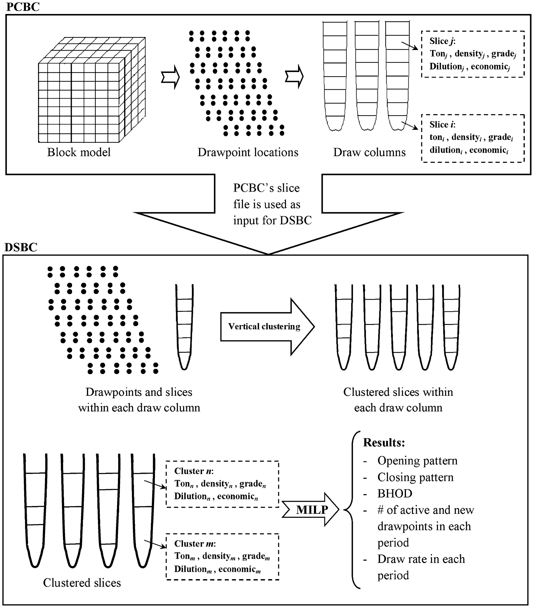
Required steps for block-cave production scheduling using the developed mixed-integer linear programming (MILP) model

Figure 1 shows the workflow that has to be followed to schedule a block-cave mine using the developed MILP model. The developed MILP model uses PCBC's (GEOVIA-Dassault, 2012) slice file as input. The first step is to create a block model in which each block represents an attribute of the geological deposit. The second step is to create a slice file. Afterwards, slices within each draw column are aggregated based on the similarity of the slices. The similarity index is defined based on economic value, dilution percentage and physical location. All the clustering and optimisation steps are carried out by a prototype software developed in-house for drawpoint scheduling in block-caving (DSBC) (Pourrahimian, 2013).

In practice, formulating a real-size mine production planning problem by including all the slices as integer variables will exceed the capacity of the current commercial mathematical optimisation solvers. An efficient way of overcoming the large number of decision variables and constraints is to apply a clustering technique. Clustering can be referred to as the task of grouping similar entities together so that maximum intra-cluster similarity and inter-cluster dissimilarity are achieved.

Various methods of aggregation have been used to reduce the number of integer variables that are required to formulate the mine-planning problem with mathematical programming (Epstein et al., 2003; Newman and Kuchta, 2007; Weintraub et al., 2008; Askari-Nasab et al., 2011; Tabesh and Askari-Nasab, 2011; Pourrahimian et al., 2012a; Pourrahimian, 2013).

In order to reduce the number of binary variables in the formulation presented here, the algorithm presented by Tabesh and Askari-Nasab (2011) was modified to aggregate slices within each draw column. The general procedure of the algorithm is as follows:

(1)

Define the maximum number of required clusters and the maximum number of allowed slices within each cluster.

(2)

Each slice is considered as a cluster. The similarities between clusters are the same as the similarities between the objects they contain.

(3)

Similarity values are calculated.

(4)

The most similar pair of clusters is merged into a single cluster.

(5)

The similarity between the new cluster and the rest of the clusters is calculated.

(6)

Steps (2) and (3) are repeated until the maximum number of clusters is reached or there is no pair of clusters to merge because of the maximum number of allowed slices within each cluster.

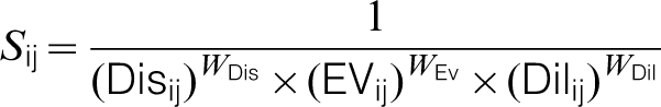
Similarity value between slices i and j, S_ij, is calculated by (1) where Dis_ij represents the normalised distance value between slices i and j, EV_ij represents the normalised economic value difference between slices i and j, and Dil_ij represents the normalised dilution difference between slices i and j. W_Dis, W_Ev, and W_Dil are weighting factors for distance, economic value and dilution, respectively. The weights are defined by the mine planner.

The economic value of each cluster (CLSEV) is equal to the summation of the economic value of the slices within the cluster and the costs incurred in mining. The CLSEV is a constant value for each cluster.

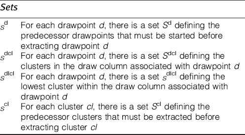
According to the advancement direction, the precedence between drawpoints is defined. For each drawpoint d there is a set S^d which defines the predecessor drawpoints among the adjacent drawpoints that must be started before drawpoint d is extracted. The set S^d is created in each advancement direction based on the presented method by Pourrahimian et al. (2012a, 2012b).

MILP model for block-cave production scheduling

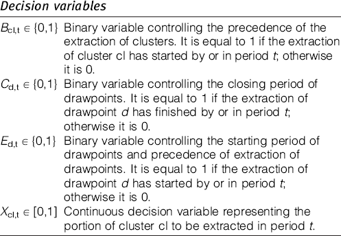
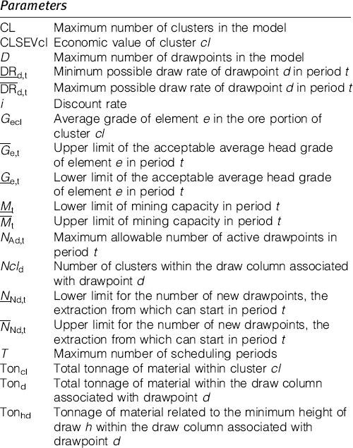
The MILP model for block-cave production scheduling optimisation is explained in this section. The notation used to formulate the problem is classified as indices, parameters, sets and decision variables. To solve the problem using the developed MILP model, one continuous decision variable and one binary variable for clusters and two binary variables for drawpoints are employed. The continuous decision variable indicates the portion of extraction from each cluster in each period. The binary variables control the number of active drawpoints, precedence of extraction between drawpoints, the opening and closing time of each drawpoint, the extraction rate from each drawpoint, the number of new drawpoints that need to be constructed in each period and precedence between clusters.

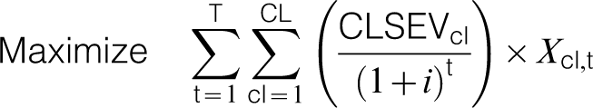
Objective function

(2)

Constraints

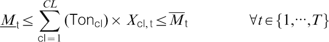
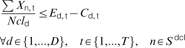
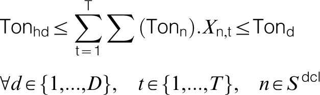
(3) (4) (5) (6) (7) (8) (9) (10) (11) (12) (13) (14) (15) (16) (17) (18) (19) Profit from mining a drawpoint depends on the value of the clusters and the costs incurred in mining. The objective function, equation (2), is composed of the CLSEV, discount rate and a continuous decision variable that indicates the portion of the cluster extracted in each period. The objective function seeks to mine clusters with higher economic value earlier than other clusters.

The constraints are presented by equations (3)–(19). Equation (3) represents the mining capacity which ensures that the total tonnage of material extracted from clusters in each period is within the acceptable range that allows flexibility for potential operational variations. The constraints are controlled by the continuous variable X_cl,t. There is one constraint per period.

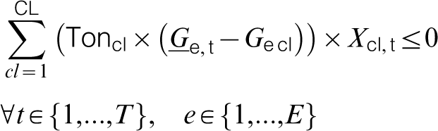
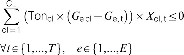
Equations (4) and (5) control the production's average grade. They force the mining system to achieve the desired grade. The average grade of the element of interest has to be within the acceptable range and between the certain values.

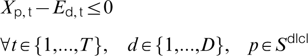
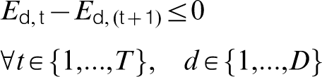
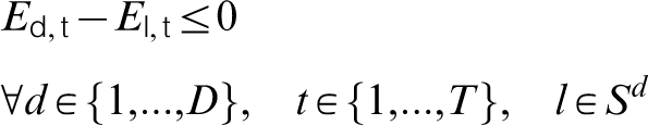
Each draw column is divided into slices. Then, slices are aggregated based on the presented clustering method. The lowest cluster in each draw column controls the starting period of extraction from the associated drawpoint. This means that the extraction from the draw column associated with drawpoint d is started by the extraction from the relevant lowest cluster. Equation (6) controls this concept and forces variable E_d,t to change to 1 when a portion of the lowest cluster of the draw column is extracted in period t. Equation (7) ensures that when variable E_d,t changes to 1, it remains 1 until the end of the mine life.

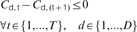
When the extraction of the last portion of a cluster is finished in period t, extraction of the cluster above can start in period t or t+1. In other words, the extraction of a cluster can start if the cluster below has been totally extracted. If the extraction of a cluster is not started after finishing the extraction of the cluster below in period t or t+1, the relevant drawpoint must be closed. The concept is applied using equation (8). This ensures that when drawpoint d is open, at least a portion of one of the clusters within the draw column associated with drawpoint d is extracted. This means extraction must be continuous; otherwise, the drawpoint will be closed. Equation (9) ensures that when variable C_d,t changes to 1, it remains 1 until the end of the mine life.

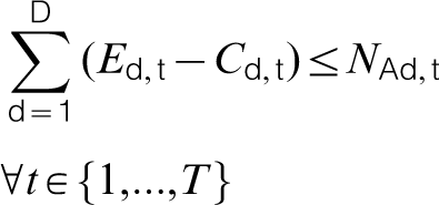
As mentioned, when variables E_d,t and C_d,t change to 1, they remain 1 until the end of the mine life. This helps us to control the maximum number of active drawpoints in each period using equation (10).

The mining precedence is controlled in vertical and horizontal directions. The precedence between drawpoints is controlled in a horizontal direction while the precedence between clusters is controlled in a vertical direction. Equation (11) ensures that all drawpoints belonging to the relevant set S^d are started before drawpoint d is extracted. This set is defined based on the selected mining advancement direction. The set can be empty, which means the considered drawpoint can be extracted in any time period in the schedule. Equation (11) also ensures that only the set of the immediate predecessor drawpoints needs to start before starting the drawpoint under consideration.

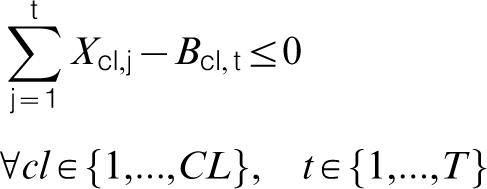
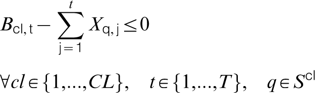
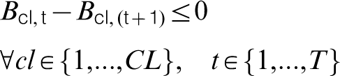
Extraction of cluster cl can be started if the cluster below it has been totally extracted. For each cluster within the draw column except the lowest, there is a set S^cl defining the predecessor cluster that must be extracted before the extraction of cluster cl. The extraction precedence of the clusters within each draw column is controlled by equations (12), (13) and (14). Equation (12) forces variable B_cl,t to change to 1 if extraction from cluster cl is started in period t. Equation (13) ensures that variable B_cl,t can change to 1 only if the cluster below it has been extracted totally. In other words, this ensures that the extraction of the slice belonging to the relevant set S^cl has been finished before the extraction of cluster cl. Equation (14) ensures that when variable B_cl,t changes to 1, it remains 1 until the end of the mine life. Equation (15) guarantees that cluster cl is extracted when the relevant drawpoint is active.

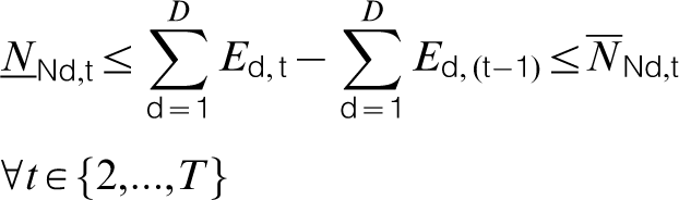
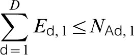
The drawpoint opening is controlled by the variable E_d,t, which takes a value of 1 from the opening period to the end of the mine life. From period 2 to the end of the mine life, the difference between the summation of opened drawpoints until and including period t and the summation of opened drawpoints until and including previous period t−1, indicates the number of new drawpoints that need to be opened in each period. Equation (16) ensures that the number of new drawpoints opened in each period except period 1 is within the acceptable range. At the beginning and in period 1, the number of new drawpoints is equal to the maximum number of active drawpoints, equation (17).

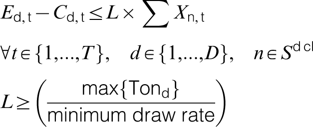
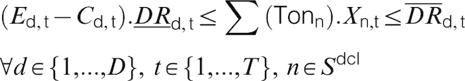
Equation (18) ensures that the draw rate from each drawpoint is within the desired range in each period. Equation (18) imposes upper and lower bounds for the draw rate. When drawpoint d is not active, (E_d,t−C_d,t) is equal to zero and this relaxes the lower bound of the equation.

In this formulation, the mining reserve is computed as a result of the optimal production schedule. Equation (19) ensures that the amount of the extracted material from drawpoint d is equal to or less than the total tonnage of the material within the draw column associated with drawpoint d. The lower bound of equation (19) is the tonnage related to the minimum HOD in each draw column associated with drawpoint d. The minimum HOD is defined by the mine planner.

Solving the optimisation problem

The proposed MILP model has been developed, implemented and tested in the TOMLAB/CPLEX environment (Holmstrom, 2011). A prototype software with a graphical user interface has been developed in-house (DSBC) in the MATLAB environment (MathWorks Inc., 2013). Drawpoint scheduling in block-caving integrates all the steps of the optimisation including setting up the input parameters, clustering, creating the objective function and constraints, and calling the CPLEX optimisation engine in one environment.

Using a branch-and-bound algorithm to solve MILP problem formulations guarantees an optimal solution if the algorithm is run to completion. Authors have used the gap tolerance (EPGAP) as an optimisation termination criterion. The gap tolerance sets an absolute tolerance on the gap between the best integer objective and the objective of the best node remaining.

The application of the model was implemented on a Dell Precision T7500 computer at 2·7 GHz, with 24 GB of RAM. The goal was to maximise the NPV at a discount rate of 12% and determine the mining reserve as a result of the optimal production schedule, while assuring that all constraints were satisfied during the mine-life.

Case study: implementation of MILP model

The performance of the proposed model is analysed based on NPV, mining production and practicality of the generated schedules. A real data set containing 102 drawpoints and 3470 slices with the slice height of 10 m is considered. The minimum and maximum numbers of slices within draw columns are 33 and 36, respectively. Figure 2 illustrates a plan view of the drawpoint configuration based on the relevant coordinates and distance between the centre-lines of draw columns. Figure 3 illustrates a 3D view of the draw columns. The total tonnage of available material is 22·5 Mt. The tonnage of draw columns varies from 203·5 to 355·5 kt. The deposit is scheduled over 14 periods.

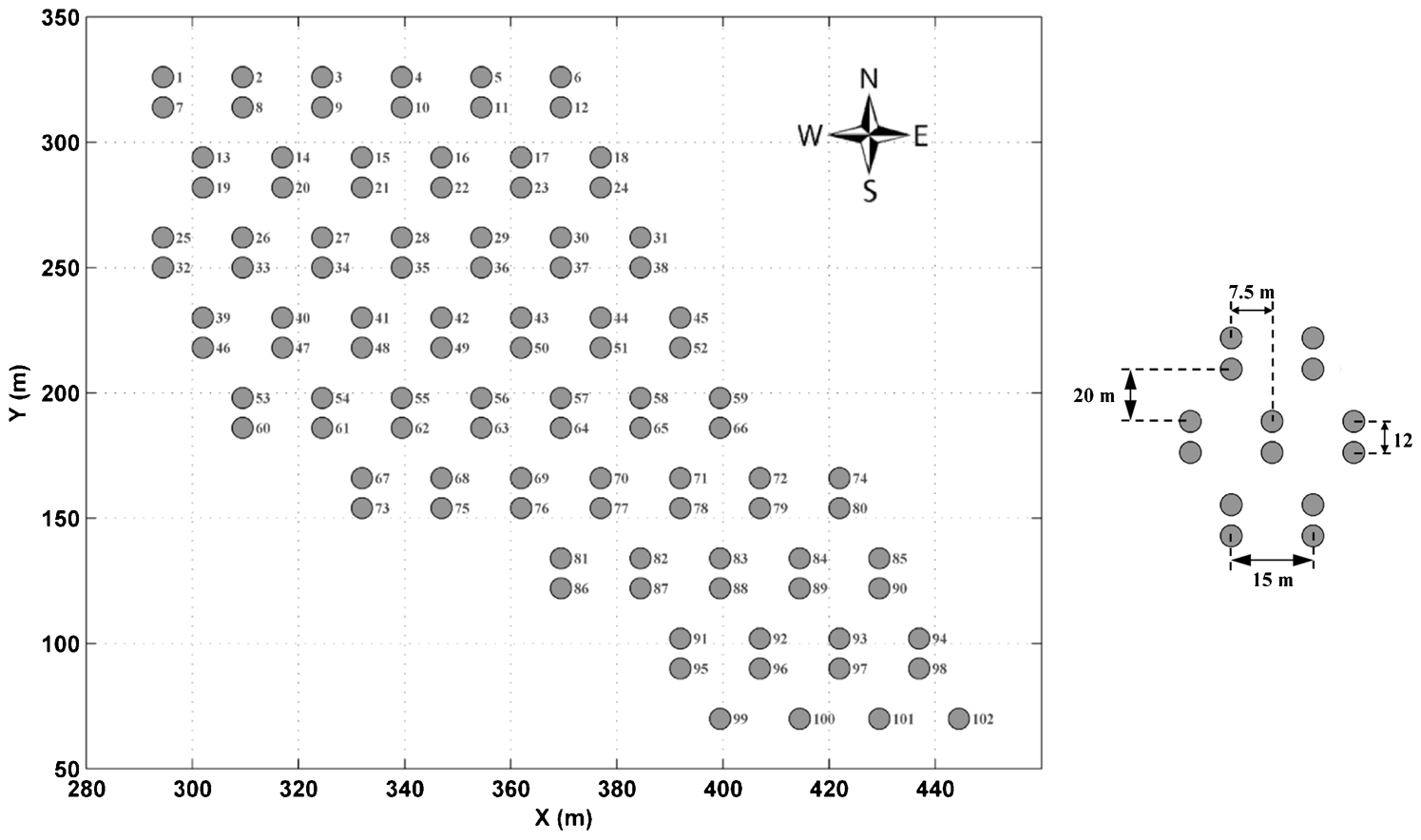
Plan view of 102 drawpoints

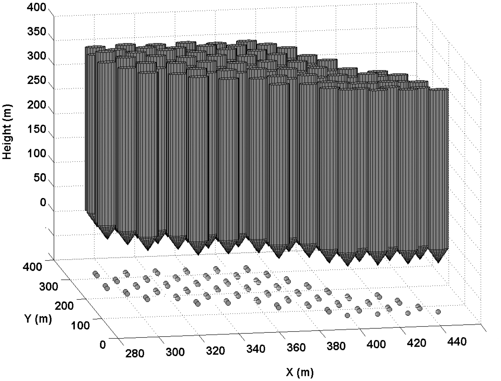
3D view of draw columns (102 draw columns)

To aggregate the slices within each draw column, the modified clustering method was applied. The weight factors of the distance, economic value and dilution were set to 5, 3, and 3, respectively. The maximum number of slices in each cluster could not be more than five. One-thousand clusters were created based on the presented algorithm. Figure 4 illustrates examples of grade distribution within two different draw columns.

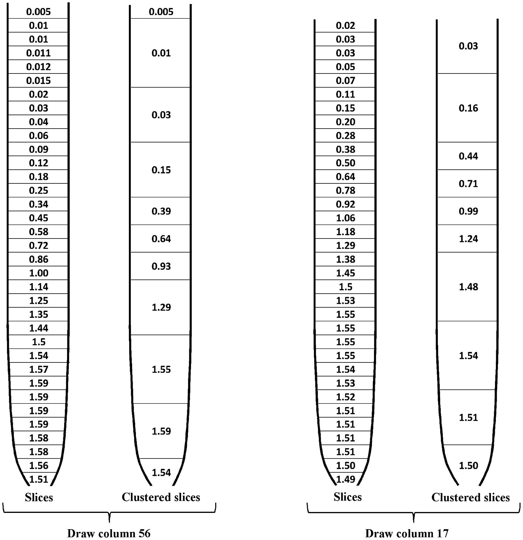
Grade distribution within draw columns 56 and 17, before and after clustering

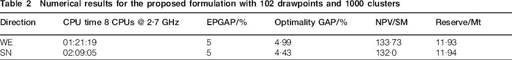
A capacity of 900 kt year⁻¹ is considered as the upper bound on the mining capacity. The maximum number of active drawpoints in each period was set to 40. The maximum number of new drawpoints which could be opened in each period was set to 15. The lower and upper bounds of the draw rate for drawpoints were set to 10 kt year⁻¹ per drawpoint and 40 kt year⁻¹ per drawpoint. The lower and upper bounds of the average grade of Copper were set to 0·8 and 1·7%.The HOD is limited to not less than 50 m. This means at least 50 m of the drawpoints must be extracted. An EPGAP of 5% was set for the optimisation run. The problem was solved for two directions, west to east (WE) and south to north (SN). Tables 1 and 2 show the number of decision variables, the number of constraints, and numerical results for both the WE and SN directions. The resulting NPVs are $133·73M and $132·0M in the WE and SN directions, respectively.

Table 1

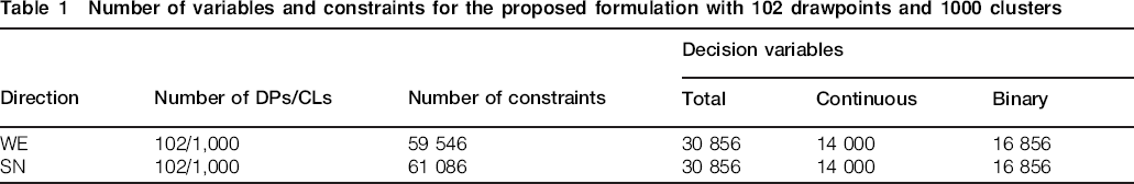
Number of variables and constraints for the proposed formulation with 102 drawpoints and 1000 clusters

Direction	Number of DPs/CLs	Number of constraints	Decision variables
			Total	Continuous	Binary
WE	102/1,000	59 546	30 856	14 000	16 856
SN	102/1,000	61 086	30 856	14 000	16 856

Table 2

Numerical results for the proposed formulation with 102 drawpoints and 1000 clusters

Direction	CPU time 8 CPUs @ 2·7 GHz	EPGAP/%	Optimality GAP/%	NPV/$M	Reserve/Mt
WE	01:21:19	5	4·99	133·73	11·93
SN	02:09:05	5	4·43	132·0	11·94

Figures 5 – 7 show that all assumed constraints were satisfied in the considered directions. Figure 5 illustrates the production tonnage in each period.

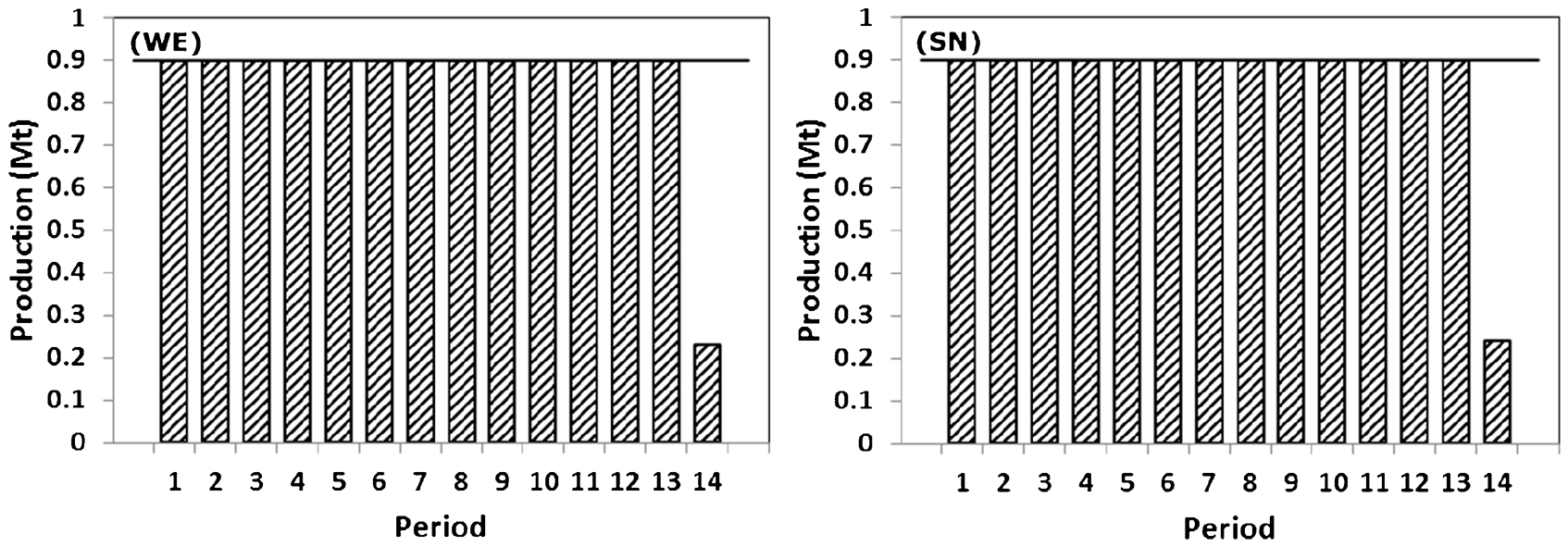
Production tonnage in the west to east (WE) and south to north (SN) directions

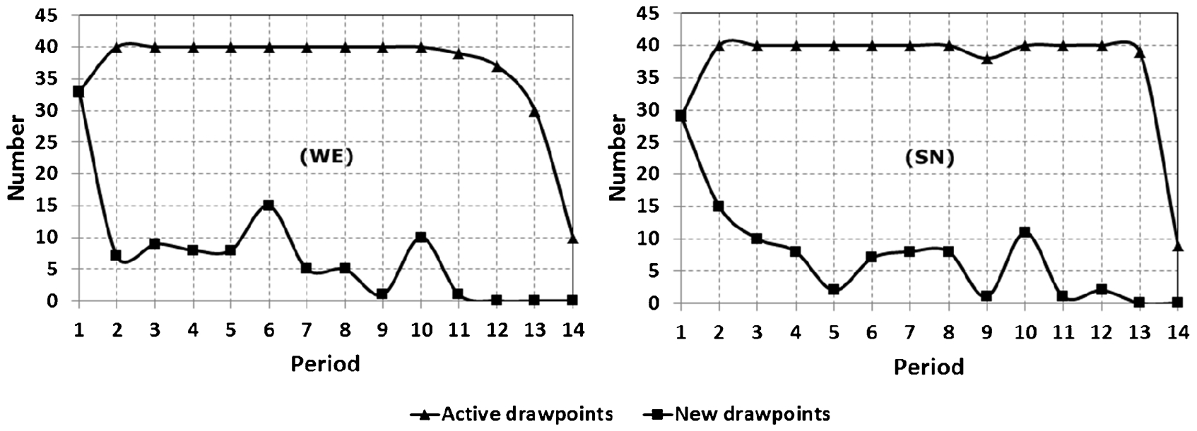
Number of active drawpoints and number of new drawpoints that must be opened in the west to east (WE) and south to north (SN) directions

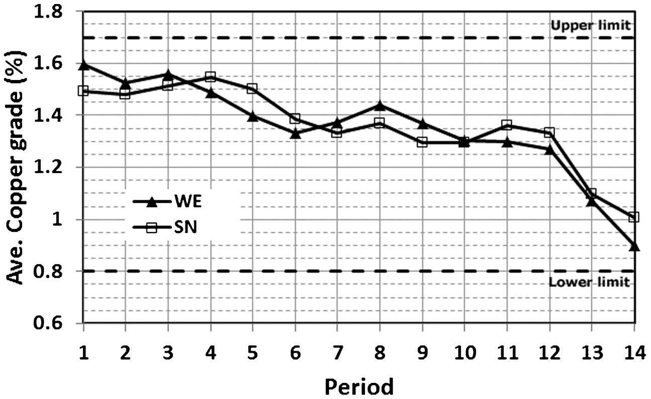
Average grade of production in the west to east (WE) and south to north (SN) directions

If mining reserve was calculated based on the BHOD (Diering, 2000) for each draw column, the total tonnage of material that could be extracted was almost 13·5 Mt, which was independent of direction. In other words, in each considered direction all the 13·5 Mt must be extracted. However in the proposed formulation, the mining reserve is computed as a result of the optimal production schedule for each advancement direction. The total tonnage of material that must be extracted in the WE and SN directions is 11·9 Mt.

Figure 6 illustrates the number of active drawpoints and the number of drawpoints that must be opened in each period. In the WE direction, the mine works with the maximum number of active drawpoints from period 2 to 10. Then, the number of active drawpoints reduces. In the SN direction, the mine works with the maximum number of active drawpoints from periods 2 to 13 except period 9. In both directions, the number of new drawpoints from periods 2 to 15 is less than 15 except in period 6 of the WE direction, in which 15 new drawpoints must be opened. In the WE direction, the last drawpoints are opened in period 11 while a number of new drawpoints are opened in period 12 in the SN direction.

Figure 7 illustrates the average grade of production. In the WE direction, during the first three periods the average grade of the production is higher than the SN direction. In both directions, during the mine life the average grade of the production was higher than 0·9%. In the SN direction, the average grade of production between periods 11 and 14 is higher than the WE direction.

Figure 8 shows the opening pattern of the drawpoints in the WE and SN directions. In the WE direction, 83% of drawpoints will be opened in the first 7 years and the rest, most of which are located at the southwest area of the mine, will be opened after period 7. In the SN direction, if the mine is divided into two sections, north and south, most of the drawpoints in the south section are opened during the first four periods.

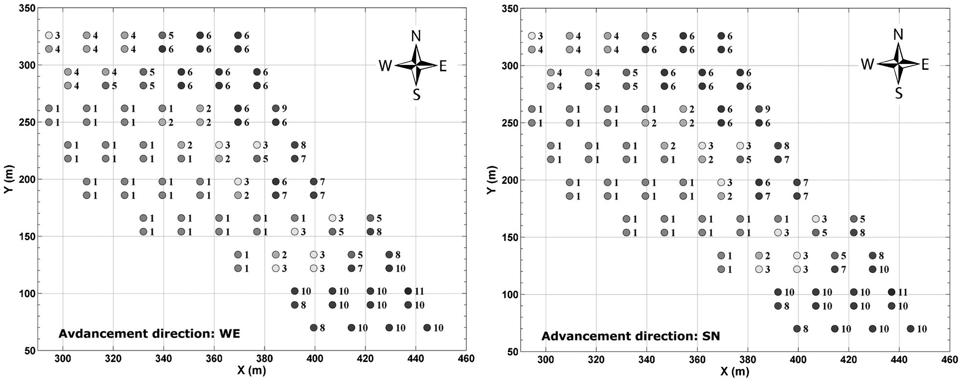
Opening pattern in the west to east (WE) and south to north (SN) directions

The possible advancement directions are defined based on geotechnical conditions. Then, using the proposed formulation, the best advancement direction and related mining reserve are computed. In the presented case study, the results are based on an optimisation termination criterion (EPGAP) of 5%. In the presented formulation, the model uses drawpoints-and-slices (Pourrahimian, 2013) in which the slices are aggregated vertically in each draw column. The considered case study was also solved without vertical clustering. The solving time for the clustered slices was 78 times faster than for the other method.

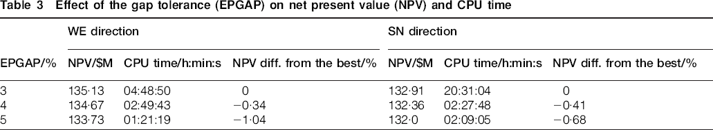
Table 3 shows the obtained NPVs and CPU times for different EPGAPs. It is obvious that when the EPGAP decreases the CPU time dramatically increases.

Table 3

Effect of the gap tolerance (EPGAP) on net present value (NPV) and CPU time

	WE direction			SN direction
EPGAP/%	NPV/$M	CPU time/h:min:s	NPV diff. from the best/%	NPV/$M	CPU time/h:min:s	NPV diff. from the best/%
3	135·13	04:48:50	0	132·91	20:31:04	0
4	134·67	02:49:43	−0·34	132·36	02:27:48	−0·41
5	133·73	01:21:19	−1·04	132·0	02:09:05	−0·68

Conclusion

This paper investigated the development of a MILP formulation for block-cave production scheduling optimisation. The presented MILP formulation developed, implemented and tested for block-cave production scheduling in the TOMLAB/CPLEX environment. The formulation maximises the NPV subject to several constraints and the mining reserve is computed as a result of the optimal production schedule. To reduce the number of binary variables and to solve the problem within a reasonable CPU time, slices within each draw column were aggregated based on the similarity index that was defined based on the slices’ distance, economic value and dilution.

The proposed formulation can be used in different advancement directions which are selected based on geotechnical considerations. Consequently, the mining reserve, which is a result of optimisation, also varies from one direction to another. The large-scale problems can be solved in a reasonable CPU time by applying the presented method here on the drawpoint-and-slice level of the multi-step method presented by Pourrahimian (2013). The concept of different cave advancement directions presented here helps planners to find the best single operation direction or combination thereof and the best starting location to reach the maximum NPV.

Production scheduling optimisation techniques are still not widely used in the mining industry. There is a need to improve the practicality and performance of the current production scheduling optimisation tools used by the mining industry. Future research will focus on modifying the approach for handling multiple-lift and multiple-mine scenarios. In addition, other efficient mathematical formulation techniques will be explored in an attempt to reduce the execution time for large-scale block-cave production scheduling.

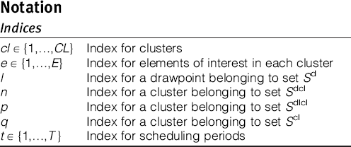
Notation

Indices

cl ∈ {1,…,CL}	Index for clusters
e ∈ {1,…,E}	Index for elements of interest in each cluster
l	Index for a drawpoint belonging to set S^d
n	Index for a cluster belonging to set S^dcl
p	Index for a cluster belonging to set S^dlcl
q	Index for a cluster belonging to set S^cl
t ∈ {1,…,T}	Index for scheduling periods

Parameters

CL	Maximum number of clusters in the model
CLSEVcl	Economic value of cluster cl
D	Maximum number of drawpoints in the model
	Minimum possible draw rate of drawpoint d in period t
	Maximum possible draw rate of drawpoint d in period t
i	Discount rate
G _ecl	Average grade of element e in the ore portion of cluster cl
	Upper limit of the acceptable average head grade of element e in period t
	Lower limit of the acceptable average head grade of element e in period t
	Lower limit of mining capacity in period t
	Upper limit of mining capacity in period t
	Maximum allowable number of active drawpoints in period t
	Number of clusters within the draw column associated with drawpoint d
	Lower limit for the number of new drawpoints, the extraction from which can start in period t
	Upper limit for the number of new drawpoints, the extraction from which can start in period t
T	Maximum number of scheduling periods
Ton_cl	Total tonnage of material within cluster cl
Ton_d	Total tonnage of material within the draw column associated with drawpoint d
Ton_hd	Tonnage of material related to the minimum height of draw h within the draw column associated with drawpoint d

Sets

_S ^d	For each drawpoint d, there is a set S^d defining the predecessor drawpoints that must be started before extracting drawpoint d
_S ^dcl	For each drawpoint d, there is a set S^dcl defining the clusters in the draw column associated with drawpoint d
_S ^dlcl	For each drawpoint d, there is a set _S ^dlcl defining the lowest cluster within the draw column associated with drawpoint d
_S ^cl	For each cluster cl, there is a set S^cl defining the predecessor clusters that must be extracted before extracting cluster cl

Decision variables

B_cl,t ∈ {0,1}	Binary variable controlling the precedence of the extraction of clusters. It is equal to 1 if the extraction of cluster cl has started by or in period t; otherwise it is 0.
C_d,t ∈ {0,1}	Binary variable controlling the closing period of drawpoints. It is equal to 1 if the extraction of drawpoint d has finished by or in period t; otherwise it is 0.
E_d,t ∈ {0,1}	Binary variable controlling the starting period of drawpoints and precedence of extraction of drawpoints. It is equal to 1 if the extraction of drawpoint d has started by or in period t; otherwise it is 0.
X_cl,t ∈ [0,1]	Continuous decision variable representing the portion of cluster cl to be extracted in period t.

References

Alford

, Brazil

and Lee

. 2007. Optimisation in Underground Mining (chapter 30). in Handbook of operations research in natural resources, international series in operations research amp; mana, International Series in operations research & management science, 561–577, Springer.

Askari-Nasab

, Pourrahimian

, Ben-Awuah

and Kalantari

2011. Mixed integer linear programming formulations for open pit production scheduling, J. Min. Sci., 47, (3), 338–359.

Brown

. 2003. Block caving geomechanics, 516. Brisbane, QLD, Julius Kruttschnitt Mineral Research Centre, The University of Queensland.

Caccetta

2007. Application of optimisation techniques in open pit mining, in Handbook of operations research in natural resources, vol. 99, international series in operations research amp; mana, (eds. Weintraub

, Romero

, Bjørndal

, Epstein

, and Miranda

), 547–559, Springer.

Chanda

ECK

. 1990. An application of integer programming and simulation to production planning for a stratiform ore body, Min. Sci. Technol., 11, (2), 165–172.

Chitombo

. 2010. Cave mining-16 years after Laubscher's 1994 paper ‘cave mining-state of the art’, in Proceedings of Caving 2010, 45–61, Perth, Australia, Australian Centre for Geomechanics.

Diering

2000. PC-BC: a block cave design and draw control system, in Proceedings of MassMin 2000, 301–335, Melbourne, Brisbane, Australia, The Australasian Institute of mining and Metallurgy.

Diering

2004. Computational considerations for production scheduling of block cave mines, in Proceedings of MassMin 2004, 135–140, Santiago, Chile.

Epstein

, Gaete

, Caro

, Weintraub

, Santibanez

and Catalan

2003. Optimizing long-term planning for underground copper mines, in Proceedings of Copper 2003, 5th International Conference, 265–279, Santiago, Chili, CIM-Chilean Institute of Mining.

10.

GEOVIA-Dassault . 2012. Ver. 6·2·4, Vancouver, BC, Canada.

11.

Guest

, VanHout

, Von

and Scheepers

. 2000. An application of linear programming for block cave draw control, in Proceedings of MassMin 2000, Melbourne, Brisbane, Australia, The Australian Institute of Mining and Metallurgy.

12.

Holmstrom

2011. TOMLAB/CPLEX, Ver. 11·2, Pullman, WA, USA, Tomlab Optimization.

13.

Kuchta

, Newman

and Topal

2004. Implementing a production schedule at LKAB's Kiruna mine, Interfaces, 34, (2), 124–134.

14.

MathWorks Inc. 2013. MATLAB (2013b), Ver. 8.2.0.701, Natick, Massachusetts, United States.

15.

Newman

and Kuchta

2007. Using aggregation to optimize long-term production planning at an underground mine, Eur. J. Oper. Res., 176, (2), 1205–1218.

16.

Newman

, Rubio

, Caro

, Weintraub

and Eurek

2010. A review of operations research in mine planning, Interfaces, 40, 222–245.

17.

Parkinson

. 2012. Essay on sequence optimization in block cave mining and inventory policies with two delivery size, PhD thesis, University of British Colombia, Vancouver, 188.

18.

Pourrahimian

2013. Mathematical programing for sequence optimization in block cave mining, PhD thesis, The University of Alberta, Edmonton, AB, Canada, 238.

19.

Pourrahimian

, Askari-Nasab

and Tannant

2012a. Mixed-integer linear programming formulation for block-cave sequence optimisation, Int. J. Min. Miner. Eng., 4, (1), 26–49.

20.

Pourrahimian

, Askari-Nasab

and Tannant

2012b. Block cave production scheduling optimization using mathematical programming, in Proc. 6th International Conf. and Exhibition on “Mass Mining (MassMin)”, 6799, Sudbury, ON, Canada.

21.

Rahal

, Smith

, Van Hout

and Von Johannides

2003. The use of mixed integer linear programming for long-term scheduling in block caving mines, in Proceedings of 31st International Symposium on the Application of Computers and operations Research in the Minerals Industries (APCOM), Cape Town, South Africa.

22.

Rubio

(2002). Long-term planning of block caving operations using mathematical programming tools, MSc thesis, University of British Columbia, Vancouver, Canada, 116.

23.

Rubio

(2006). Block cave mine infrastructure reliability applied to production planning, PhD thesis, University of British Columbia, Vancouver, 132.

24.

Rubio

and Diering

2004. Block cave production planning using operations research tools, in Proceedings of MassMin 2004, 141–149, Santiago, Chile.

25.

Song

(1989). Caving process simulation and optimal mining sequence at Tong Kuang Yu mine, China, in Proceedings of 21st Application of Computers and Operations Research in the Mineral Industry, Society of mining Engineering of the American Institute of Mining, Metallurgical, and Petroleum Engineers, Inc., 386–392, Littleton, CO, Las Vegas, NV, USA.

26.

Tabesh

and Askari-Nasab

2011. Two-stage clustering algorithm for block aggregation in open pit mines, Min. Technol., 120, (3), 158–169.

27.

Topal

2008. Early start and late start algorithms to improve the solution time for long-term underground mine production scheduling, J. S. Afr. Inst. Min. Metall., 108, (2), 99–107.

28.

Weintraub

, Pereira

and Schultz

2008. A priori and a posteriori aggregation procedures to reduce model size in MIP mine planning models, Electron. Notes Discrete Math., 30, 297–302.

29.

Winkler

and Griffin

1998. Mine production scheduling with linear programming-development of a practical tool, in Proceedings of 27th International Symposium, Application of Computers in the Mineral Industry (APCOM), 673–679, London, United Kingdom, Institution of Mining and Metallurgy.