Incorporating fine-scale ground-penetrating radar data into the mapping of lateral variability of a laterite-type bauxite horizon

Abstract

Ground-penetrating radar (GPR) offers an inexpensive and rapid method for delineating the laterite profiles by acquiring fine-scale data from the ground. In a case study, a GPR survey was conducted at the Weipa bauxite mine in Australia, in which numerous pick points corresponding to the depth to the bauxite/ironstone boundary were acquired from the ground. These pick points were subsequently merged with the available exploration borehole data using four prediction algorithms, including standard linear regression (SLR), simple kriging with varying local means (SKLM), Bayesian integration (BAY), and ordinary co-located cokriging (OCCK). The required structural inputs for the aforementioned algorithms were derived from the modelled auto and cross-semi-variograms. The cross-validation results suggest that the SKLM approach yielded the most robust estimates. The comparison of these estimates with the actual mine floor also indicates that the inclusion of ancillary GPR data substantially improved the estimation quality.

Keywords

Geostatistics Ground-penetrating radar Laterite Bauxite Ironstone Weipa

Introduction

The tropical laterite-type bauxite deposits often pose a unique challenge to resource modelling and mine planning because of the extreme lateral variability of the weathering profile (Bardossy and Aleva, 1990). The base of the lateritic bauxite deposit tends to be sufficiently variable that the economically viable drilling grid is frequently greater than the spatial frequency of the variations in the profile thickness (Francke, 2012b; Singh, 2007). Thus, accurate volume estimates are difficult to derive based solely on the widely spaced borehole data. However, the prediction of horizon continuity is of critical importance in terms of both mine planning and alumina (Al₂O₃%) refinery efficiency (Erten, 2012). At Weipa, the current drilling grid (76·2×76·2 m) was chosen based heavily on the knowledge of the continuity and variation in alumina (Al₂O₃%) grade (Morgan, 1993). However, the robustness of the resource model depends more on the reliable thickness estimate than grade estimate at laterite-type bauxite deposits. Abzalov and Bower (2009) also postulated that the alumina (Al₂O₃%) grade distribution could be accurately estimated throughout the entire Weipa deposit using sparsely spaced borehole data. However, they also mention that the optimal borehole spacing determined for the measured and indicated resources is rather insufficient for a robust grade control at the time of mining. Hence, an accurate prediction of the bauxite/ironstone horizon surface is required to construct a reliable resource model, as this horizon surface is generally used to geologically constrain the block model.

Geostatistics, which is based on the theory of regionalised variables, is used to interpolate between the sampled points and to estimate the unsampled points as a linear weighted combination of samples within a predefined search neighbourhood (Chiles and Delfiner, 1999; Goovaerts, 1997; Isaaks and Srivastava, 1989; Journel and Huijbregts, 1978). However, a major drawback of the geostatistical prediction algorithms is that they tend to smooth out the actual spatial structure to provide an estimate with a minimum error variance (Matheron, 1963). This inherent smoothing effect is simply described as the reduction in spatial variance of estimated values compared with true values (ASTM D 5923-96, 2004; Yamamoto, 2008). Considering the case of lateritic bauxite mines in which boreholes are generally widely spaced, the inherent smoothing effect tends to increase even further away from data locations. Therefore, kriging estimates are locally accurate; that is, near the data locations the estimates are close to reality, but do not reflect the spatial variability modelled by the covariance (Dowd, 1997; Journel et al., 2000). To alleviate the inherent smoothing effect of kriging, different sources of data that represent the same phenomenon of interest can be used to enrich the available database.

Geophysical methods can provide ideal tools for the assessment of ore continuity, grade estimation, and ore body delineation (Campbell, 1994; Fallon et al., 1997). Of the geophysical subsurface imaging techniques, ground-penetrating radar (GPR), in particular, has recently gained greater acceptance in the mining industry because of its high-resolution and fast data acquisition capabilities (Davis and Annan, 1989). GPR has increasingly been used to acquire fine-scale complementary information about bauxite and nickel laterite profiles (Barsottelli-Botelho and Luiz, 2011; Francke, 2012a; Francke and Nobes, 2000; Francke and Parkinson, 2000; Watts, 1997). Once GPR data have been acquired from the ground of a survey area, the raw data must be processed and converted from the time domain to the depth domain (Keary and Brooks, 1994).

Considering the natures of the borehole and the GPR data, borehole data are quasi-point supports, whereas GPR data represent considerably larger fuzzy volumes. Hence, it is imperative that the GPR pick points be calibrated to the co-located (zero lag) borehole data before spatial prediction. This is mainly because the prediction performance of multivariate prediction techniques is based heavily on the strength of the linear correlation between the samples of primary and secondary variables at co-located locations (Erten, 2012). The complementary geophysical information can be incorporated into the kriging procedure using multivariate geostatistical modelling techniques, such as simple kriging with varying local means (SKLM), ordinary co-located cokriging (OCCK), ordinary cokriging (OCK), kriging with external drift (KED), and Bayesian integration (BAY) (Bardossy et al., 1986; Bourennane and King, 2003; Dowd and Pardo-Iguzquiza, 2006; Doyen, 1988; Erten et al., 2013; Kay and Dimitrakopoulos, 2000; Xu et al., 1992).

This study uses four interpolation techniques, including standard linear regression (SLR), SKLM, BAY, and OCCK, to predict the lateral variability in the base of the bauxite ore unit within the Kumbur mine area at the Weipa bauxite mine in Australia. The semi-variances required for each technique are inferred from the structural analyses. The performance of each technique is assessed by cross-validation. Ordinary kriging (OK), which only uses the borehole data in the estimation process, is used as a benchmark that can reflect the improved performance of the estimators when the exhaustively sampled GPR pick points are integrated into the estimation process. Finally, the estimates are compared with the actual mine floor defined by the front-end loader operation.

Methodology

Geostatistical modelling

Geostatistics assumes that the data observed at spatial locations {u_α; α = 1,…,n}, are a partial realisation of a random function (RF) {Z(u):u∈D}, where u is a spatial index and D is a fixed domain in ℜ² and ℜ³. Given the modelling and estimation, the theoretical variogram is defined through the intrinsic hypothesis (Cressie, 1993), where the mean, m, is constant and the variogram, 2γ(h), depends only on the separation vector h and not on the location u (Myers, 1989) (1) (2)

However, the covariance function, C(h), is defined by the stationarity of the first two moments (mean and covariance) of RF (Journel and Huijbregts, 1978) (3) (4)

Provided that the variable, Z, is a second-order stationary RF Z(u), there is a linear relation between the covariance function, C(h), and the semi-variogram, γ(h) (5)

Various statistical and geostatistical methods are available for incorporating dense secondary information into the spatial prediction of the primary variable. Let {z(u_α),α = 1,…,n} be the primary data sampled at n locations and y(u) be the secondary data available at all primary data locations u_α and at all locations u being estimated. The most straightforward prediction approach would be the SLR method (Wackernagel, 2002), in which the primary variable, Z, is predicted as a function of the co-located secondary variable, Y. The linear relation is defined by the following equation (6) where and are the regression coefficients predicted from the set of co-located primary and secondary data {(z(u_α),y(u_α)),α = 1,…,n} (Goovaerts, 2000). The residual (error) variance, , is estimated through the following equation (7) where is the residual variance, z(u_α) is the data value co-located with y(u_α), z*(u_α) is the estimated value, and n is the number of data points where both types of data are available. The estimation variance, , is then defined by the following equation (8) where is the estimation variance, y(u_β) represents data values non-co-located with z(u_α), and y(u_α) represents data values co-located with z(u_α) (Ahmed and De Marsily, 1987; Davis, 2002).

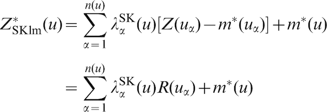
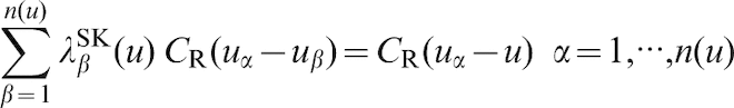
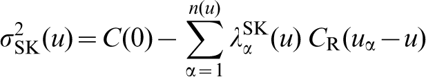
In the SKLM approach, the local mean of the primary variable Z is derived from the secondary variable Y using the SLR model E[Z(u)] = f(y(u)) = m*(u) (Goovaerts and Kerry, 2010; Odeh et al., 1995). The SKLM estimate is then expressed as a linear combination of the neighbouring primary variable observations z(u_α) and the local mean m*(u_α) estimated at n locations and the location u being predicted (9) where R(u_α) = Z(u_α) − m*(u_α) represents regression residuals. 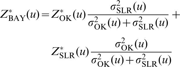The simple kriging (SK) weights are obtained from the following equation (10) where C_R(h) is the covariance function of the residual RF R(u). The estimation variance is defined by the following equation (11)

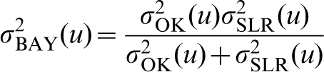
Given the BAY approach, three estimates of Z(u) are considered at each grid node: (1) the likelihood distribution, which is given by the regression estimate, and regression variance (2) the prior distribution, which is given by the primary data {z(u_α),α = 1,…,n}, OK estimate , and estimation variance ; and (3) BAY combines the likelihood and prior distributions to yield the updated distribution. To simplify the process, the prior and likelihood distributions are assumed to be Gaussian (Dowd and Pardo-Iguzquiza, 2006; Doyen et al., 1996). The BAY estimator is defined by the following equation (12)

The estimation variance is given by the following equation (13)

The OCCK approach is a variant of full cokriging, where the secondary variable Y is retained both at the sample locations of the primary variable Z and at the point being estimated within the search neighbourhood (Chiles and Delfiner, 1999; Rivoirard, 2001). The inference requirement for the OCCK estimator is the estimation of co-variances C_Z(h) and C_Y(h), and cross-covariance C_ZY(h). Consider two correlated spatial RFs, Z₁(u) and Z₂(u) corresponding to primary and secondary variables, respectively. The OCCK estimator of Z₁ at the location u is given by the following equation (14)

The kriging weights are obtained from the following equation (15)

Case study

Location and landscape background

The Weipa bauxite mine is located at approximately 12°40′S latitude and 141°30′E longitude on the northwest coast of the Cape York Peninsula in northern Queensland, Australia (Fig. 1).

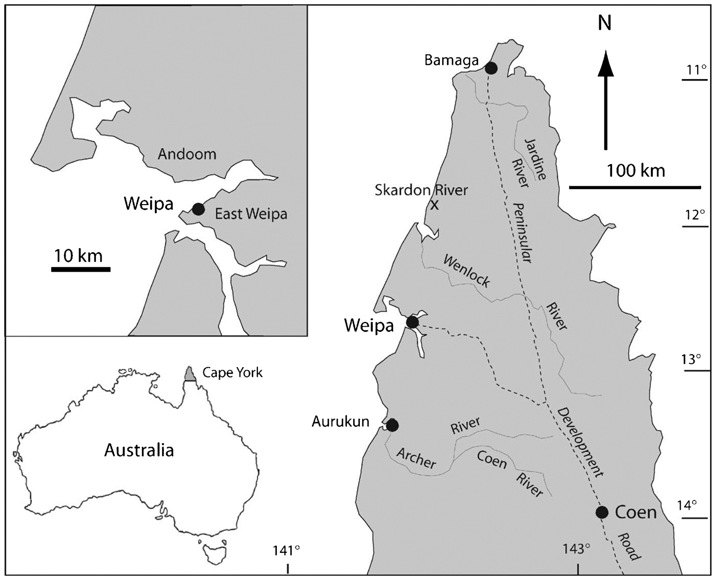
Location of the Weipa bauxite mine. After Taylor et al. (2008a)

The mine is divided into two major mine sites, namely Andoom and East Weipa, by the Mission river. The elevations of the Weipa Plateau vary from close to sea level in the West to approximately 80 m in the East (Taylor and Eggleton, 2004), and the landscape across the region consists of very gently rolling hills with discontinuous drainages in many parts (Taylor et al., 2008a). The bauxite at Weipa covers approximately 10 000 km² of western Cape York Peninsula to a depth between 1 and 6 m (Evans, 1975; Morgan, 1992a; Schaap, 1990; Taylor et al., 2008b). The surface is almost uninhabited and consists of a flat, low-lying eucalyptus forest and grassland (Morgan, 1992a), and the soils of the majority of the plateau are predominantly bauxitic dystrophic red kandosols (base-poor red earths) and bauxitic dystrophic yellow kandosols (yellow earths) (Isbell, 1983; McKenzie et al., 2004; Taylor et al., 2008a). The climate is hot and monsoonal, with temperatures varying from 30°C to 35°C during the wet and dry seasons (Evans, 1975). The annual average rainfall is 1,600 mm and falls mostly in the period from December to March (Eggleton and Taylor, 2005; Loughnan and Bayliss, 1961; McDonald and Mandla, 1993).

Geology and tectonic setting of the Weipa bauxite deposit

The Weipa bauxite deposits are formed as a result of in situ weathering of underlying Cretaceous and Palaeogene sediments (Evans, 1975; Loughnan and Bayliss, 1961; Schaap, 1990). As for the regional geology, the northern end of the Cape York Peninsula is composed of a Proterozoic and Palaeozoic basement to the East overlain by Mesozoic and Cainozoic sediments to the West. Along the northwest coast, the sediments have been intensively weathered, which leads to the formation of aluminous laterites and bauxites underlain by an almost completely kaolinised pallid zone. The basement consists principally of acidic intrusives and extrusives, as well as metamorphics, which crop out in the Eastern part of the Peninsula. The Mesozoic sediments, which are part of the Carpentaria Basin succession and dip gently to the West, are approximately 800 m thick at the West coast and consist of a sequence of quartz sandstones and conglomerates overlying marine claystones, mudstones, siltstones, and lithic sandstones derived from a predominantly andesitic province to the south. The Cainozoic sediments are superficial, fluviatile, largely arenaceous deposits formed from the basement and arenaceous Mesozoic rocks to the East on the Peninsula. The area has been tectonically stable since the bauxites were formed (Bardossy and Aleva, 1990; Morgan, 1992a).

The weathering profile of the Weipa plateau exhibits an idealised laterite-saprolite profile, including a sequence from parent rock to saprolite, plasmic zone, mottled zone, a ferruginous zone and pisolithic bauxite (Bardossy and Aleva, 1990; Eggleton, 2001; Eggleton and Taylor, 1998). The generalised profiles for Weipa and Andoom, which are provided by Morgan (1996) and Taylor et al. (2008a), are illustrated in Fig. 2.

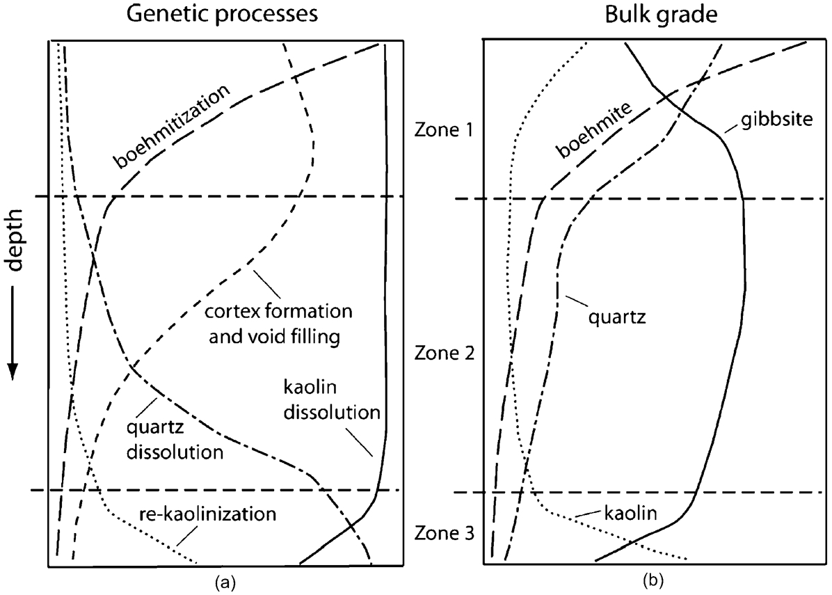
a Variation in regolith processes and b ore grade in a Weipa plateau bauxite profile. After Taylor et al. (2008a)

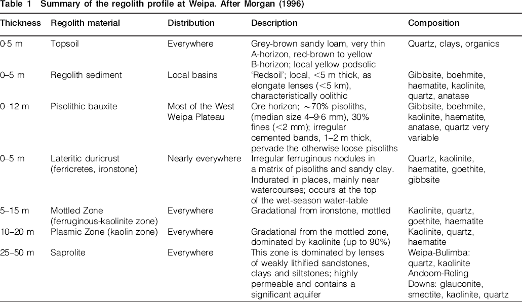
The major textural and mineralogical variations in the Weipa plateau regolith profile are indicated in Table 1.

Table 1

Summary of the regolith profile at Weipa. After Morgan (1996)

Thickness	Regolith material	Distribution	Description	Composition
0·5 m	Topsoil	Everywhere	Grey-brown sandy loam, very thin A-horizon, red-brown to yellow B-horizon; local yellow podsolic	Quartz, clays, organics
0–5 m	Regolith sediment	Local basins	‘Redsoil’; local, <5 m thick, as elongate lenses (<5 km), characteristically oolithic	Gibbsite, boehmite, haematite, kaolinite, quartz, anatase
0–12 m	Pisolithic bauxite	Most of the West Weipa Plateau	Ore horizon; ∼70% pisoliths, (median size 4–9·6 mm), 30% fines (<2 mm); irregular cemented bands, 1–2 m thick, pervade the otherwise loose pisoliths	Gibbsite, boehmite, kaolinite, haematite, anatase, quartz very variable
0–5 m	Lateritic duricrust (ferricretes, ironstone)	Nearly everywhere	Irregular ferruginous nodules in a matrix of pisoliths and sandy clay. Indurated in places, mainly near watercourses; occurs at the top of the wet-season water-table	Quartz, kaolinite, haematite, goethite, gibbsite
5–15 m	Mottled Zone (ferruginous-kaolinite zone)	Everywhere	Gradational from ironstone, mottled	Kaolinite, quartz, goethite, haematite
10–20 m	Plasmic Zone (kaolin zone)	Everywhere	Gradational from the mottled zone, dominated by kaolinite (up to 90%)	Kaolinite, quartz, haematite
25–50 m	Saprolite	Everywhere	This zone is dominated by lenses of weakly lithified sandstones, clays and siltstones; highly permeable and contains a significant aquifer	Weipa-Bulimba: quartz, kaolinite Andoom-Roling Downs: glauconite, smectite, kaolinite, quartz

The contact between the bauxite ore unit and underlying ironstone soil is believed to be formed by the precipitation of dissolved Fe²⁺ and corresponds to the position of the groundwater table at the time when the bauxite was formed (Evans, 1975; Morgan, 1996; Schaap, 1990). Evans (1965) postulated that the pisolithic bauxites were formed in a zone affected by water-table fluctuations, while the nodular and tabular zones formed in permanently saturated zones. Undulations occurring at the bauxite/ironstone interface are large and irregular, with a wavelength on a regional scale of approximately 100 m and amplitude of up to 3 m. It has also been observed that local irregularities occur at a 1–2 m scale, both in position and amplitude (Evans, 1975; Morgan, 1996). Evans (1975) also suggested that undulations at the base of the bauxite ore unit are caused by folding, which is rather common in stratified deposits.

Considering the petrophysical properties of the regolith profile at Weipa, the bauxite pisoliths tend to have low dielectric values because of their high porosity. The ironstone, on the other hand, has a lower porosity that results in higher dielectric permittivity. The ironstone also tends to have higher clay content and conductivity, which result in signal attenuation. Because of the strong increase in dielectric permittivity and conductivity in the ironstone, electromagnetic waves reflect off the contact between the bauxite ore and underlying ironstone (Morgan, 1995).

GPR data acquisition at the Kumbur mine area

Given the petrophysical properties of the laterite profile and site-specific conditions, GPR was selected to be the most appropriate technique for mapping the laterite profile at Weipa (Erten, 2012; Morgan, 1995). GPR is a geophysical subsurface imaging technique that uses propagating electromagnetic waves that respond to changes in electromagnetic properties, such as the dielectric permittivity, conductivity and magnetic permeability of the shallow subsurface (ASTM D 6432-99, 2005; Baker et al., 2007). Electromagnetic waves are radiated into the ground from a transmitting antenna at the surface. Once the propagating electromagnetic waves encounter any contrast in electrical properties, they reflect off the interface of the subsurface materials. The reflected signal is then received by a receiving antenna and recorded as a function of time (Davis and Annan, 1989).

The Kumbur mine area is located in the Ely mine site (northeast Andoom) and covers an area of approximately 215×500 m, as shown in Fig. 3. Prior to the survey, the ground of the Kumbur mine area was first bulldozed to remove all of the vegetation and topsoil. This ensured that the transmitting and receiving antennae were in direct contact with the surface, to provide maximum antennae-to-ground coupling during the survey. The extensive GPR survey was then conducted on the ground of the Kumbur mine area using a radar device (UltraGPR) with an 80-MHz GPR antennae. The UltraGPR radar system is a portable, robust digital instrument that uses an integrated real-time kinematic differential global positioning system that allows continuous subsurface data acquisition throughout the survey (Francke and Utsi, 2009).

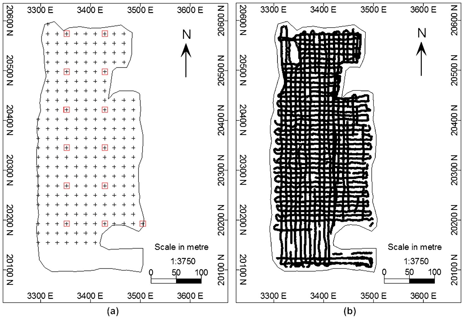
The Kumbur mine area: locations of a production control (PC) and exploration boreholes and b GPR pick points

The surveying strategy consisted of towing the UltraGPR radar system by a single person at fast walking pace along the virtual grids of the Kumbur mine area. The high-resolution subsurface digital data were acquired from the ground in a systematic manner using north-south and east-west parallel continuous profiles separated by fixed distances. The straightness of the GPR profiles was continuously checked by the tower during the surveys through the graphical display of the virtual grids on a hand held GPS device. The GPR survey at the Kumbur mine area covered an area of 67 800 m² with 15 170 m of GPR profiles. The base of the bauxite horizon was sampled every 1-m along the profiles, which provided 60 450 GPR pick points distributed along the profiles at 9 m intervals (Erten, 2012). Considering the sparsely spaced borehole data (76·2×76·2 m), the GPR data are relatively dense, which could supplement the borehole data for predicting the lateral variability of the bauxite/ironstone interface within the Kumbur mine area.

Data preparation

At Kumbur, the available borehole data comes from 13 exploration (76·2×76·2 m) and 224 production control (PC) boreholes (19·05×19·05 m), which were vertically drilled on a regular grid throughout the mine area. Given the acquired GPR data, after processing and removing duplicates, the number of GPR pick points that were used in the spatial prediction is 48 622. The locations of exploration and PC boreholes, which are denoted by red squares and plus signs, respectively, as well as the GPR pick points, are presented in Fig. 3. As seen from Fig. 3b, the distribution of GPR pick points is rather regular and is consistent with the area where the boreholes are located.

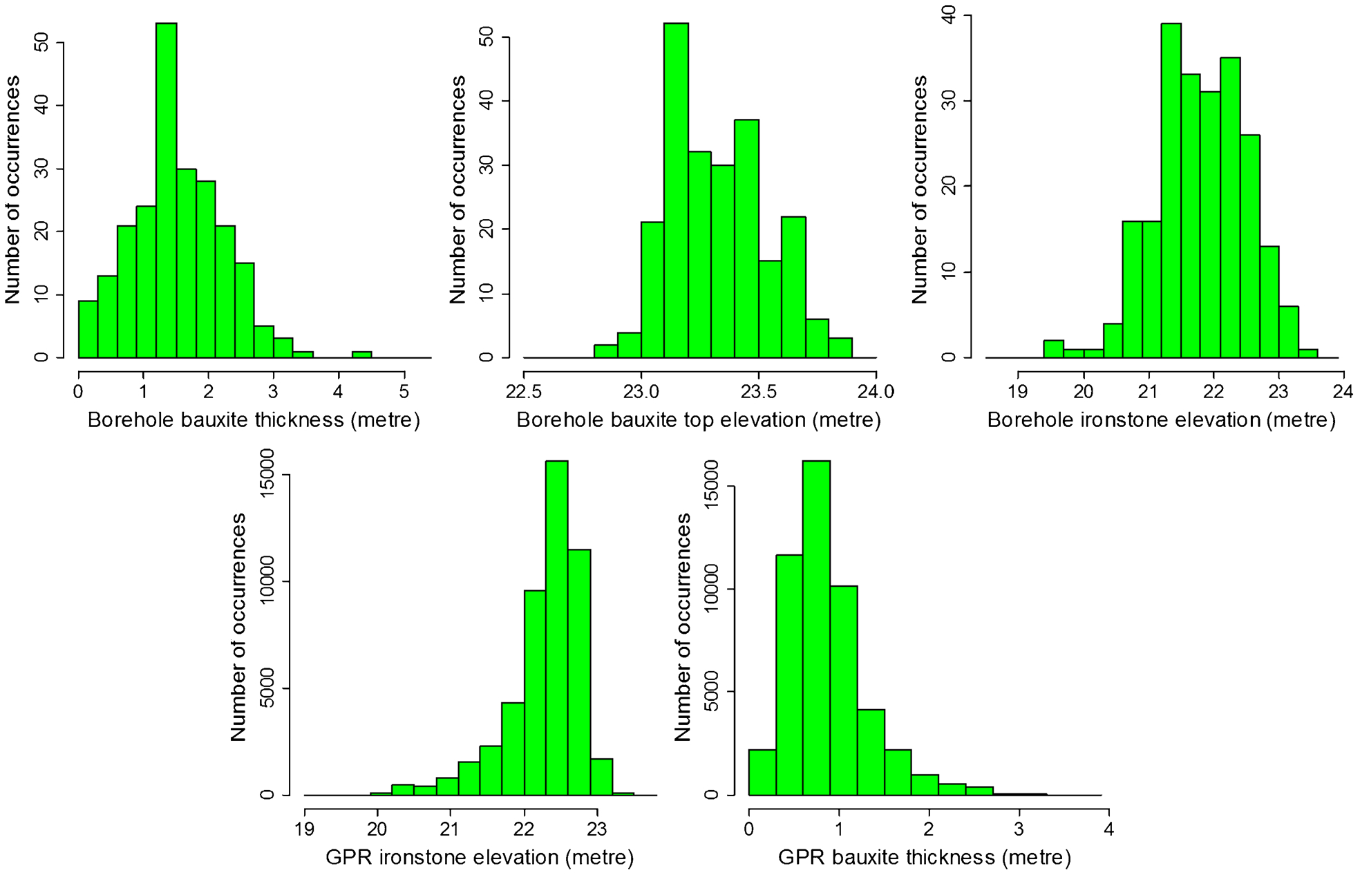
At the Weipa bauxite mine, the lithology codes assigned to each core sample based on Al₂O₃% and SiO₂% cutoff grades are used for the grade estimation. A typical complete regolith profile at Weipa is generally subdivided, from top to bottom, into five lithology codes, including ‘O’ (overburden), ‘R’ (red soil), ‘B’ (bauxite), ‘X’ (transitional zone) and ‘Z’ (ironstone) (Erten, 2012; Morgan, 1992b). Because the objective in this case study is to predict the lateral variability of the bauxite/ironstone interface, the lithology codes assigned to each core sample were employed to generate both the PC and exploration borehole elevation data, which include the bauxite top elevation, ironstone elevation (bauxite bottom elevation), and bauxite thickness variables. The available GPR data also include GPR ironstone elevation (depth to the base of bauxite ore unit) and GPR bauxite thickness variables. The histograms of PC borehole and GPR elevation data variables, which were plotted in R Software, are presented in Fig. 4.

Histograms of the PC borehole and GPR elevation data variables

As shown in Fig. 4, the histograms of PC borehole elevation data variables exhibit slightly skewed distributions, whereas the GPR elevation data variables exhibit highly skewed distributions with coefficients of skewness varying from −1·46 to 1·33. The descriptive statistics of the PC and exploration borehole and GPR elevation data variables are summarised in Table 2.

Table 2

Descriptive statistics of the PC and exploration borehole, as well as GPR elevation, data variables

Variable	Unit	Count	Mean	SD	Min	Max	CV
Exploration borehole ironstone elevation	m	13	21·75	0·53	20·63	22·69	0·02
Exploration borehole bauxite thickness	m	13	1·63	0·62	0·75	3·25	0·38
Exploration borehole bauxite top elevation	m	13	23·38	0·20	23·16	23·38	0·01
PC borehole ironstone elevation	m	224	21·80	0·70	19·45	23·35	0·03
PC borehole bauxite thickness	m	224	1·54	0·72	0·00	4·25	0·47
PC borehole bauxite top elevation	m	224	23·33	0·21	22·88	23·88	0·01
GPR bauxite thickness	m	48,622	0·87	0·44	0·04	3·26	0·51
GPR ironstone elevation	m	48,622	22·29	0·51	19·95	23·35	0·02

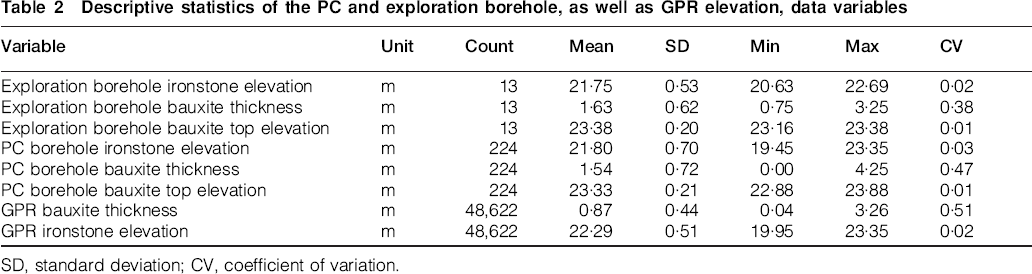
SD, standard deviation; CV, coefficient of variation.

Structural analysis

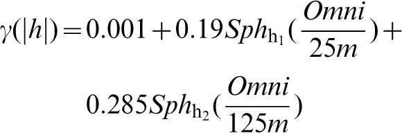
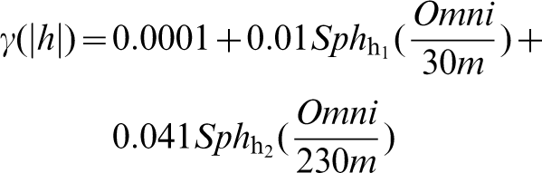
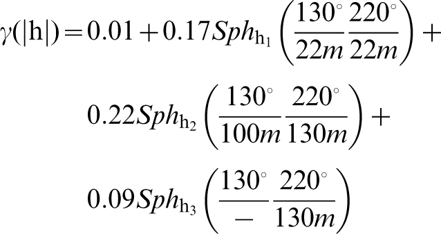
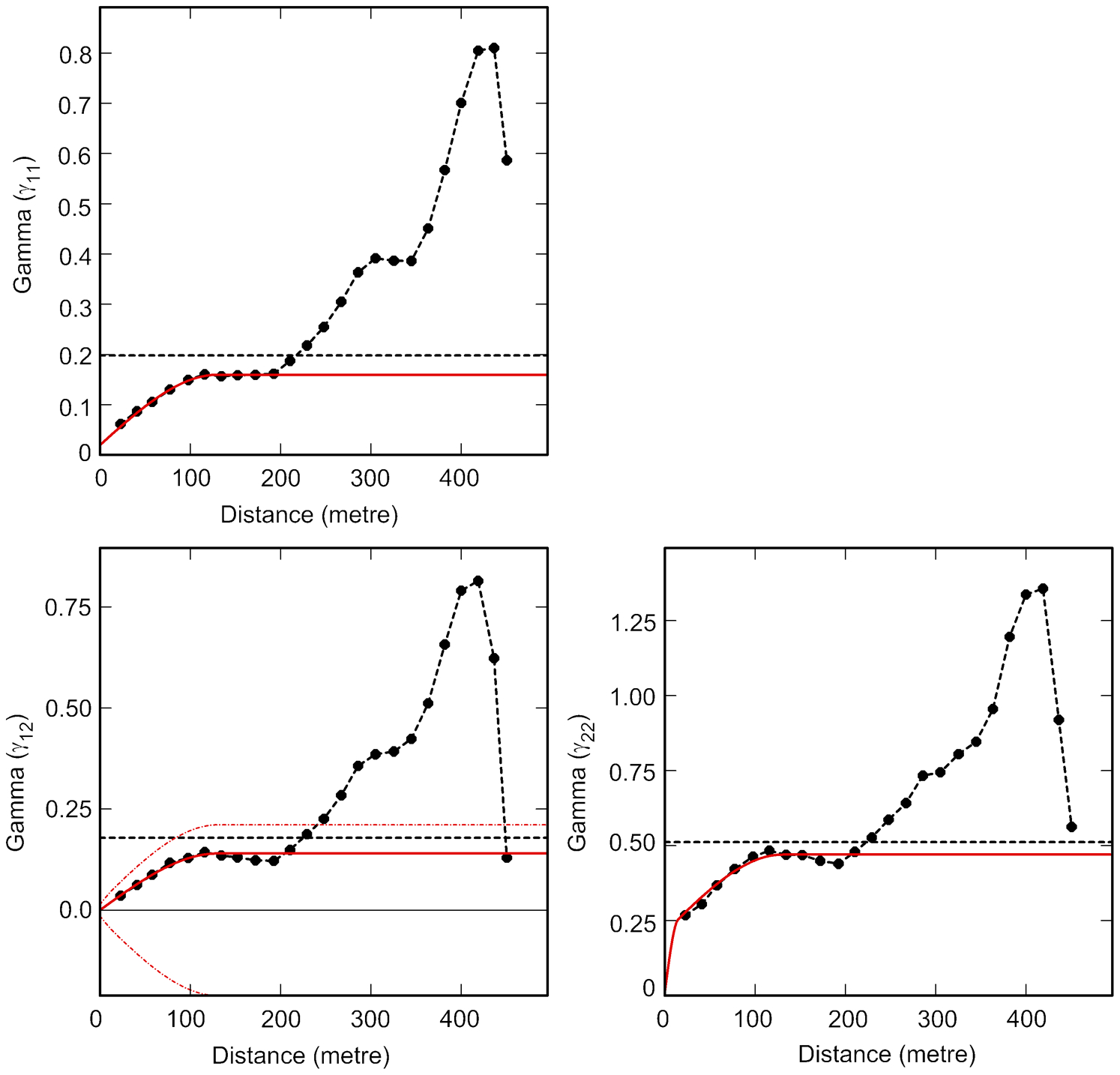
Due to the structural input required for the geostatistical prediction algorithms, the number of exploration borehole elevation data points was not sufficient to compute robust semi-variograms. Therefore, under the assumption of stationarity (Myers, 1989), all of the PC borehole elevation data were used to compute the experimental semi-variograms of both the exploration and PC borehole elevation data variables. Of the PC borehole elevation data variables, no anisotropy was detected for bauxite thickness and bauxite top elevation variables; hence, the omni-directional semi-variograms were used only to infer the required covariance values. Because of the zonal anisotropy evident in the PC borehole ironstone elevation variable data, the semi-variogram was computed along the major horizontal directions of continuity, as presented in Fig. 5. ISATIS software (Paris School of Mines and Geovariances, Fontainbleau) was used for all the structural analyses of the Kumbur data set. As for the GPR data variables, the GPR bauxite thickness and GPR ironstone elevation variables exhibit non-stationarity. Hence, the universal kriging (UK) approach (Matheron, 1971; Pardo-Iguzquiza and Dowd, 1998) was used to account for the underlying trend. The methodology described by Chihi et al. (2000) was used to compute the residual semi-variograms. The boundaries of the zone in which the GPR ironstone elevation and GPR bauxite thickness variables were stationary were first defined. Then, the data falling in these zones were used to compute residual semi-variograms of GPR ironstone elevation and GPR bauxite thickness variables. As described in equation (9), the SKLM approach uses regression residuals {R(u_α),α = 1,…,n} in the kriging system. The semi-variogram of the residuals for the borehole bauxite thickness variable was computed for use as a structural input in the SKLM kriging system.

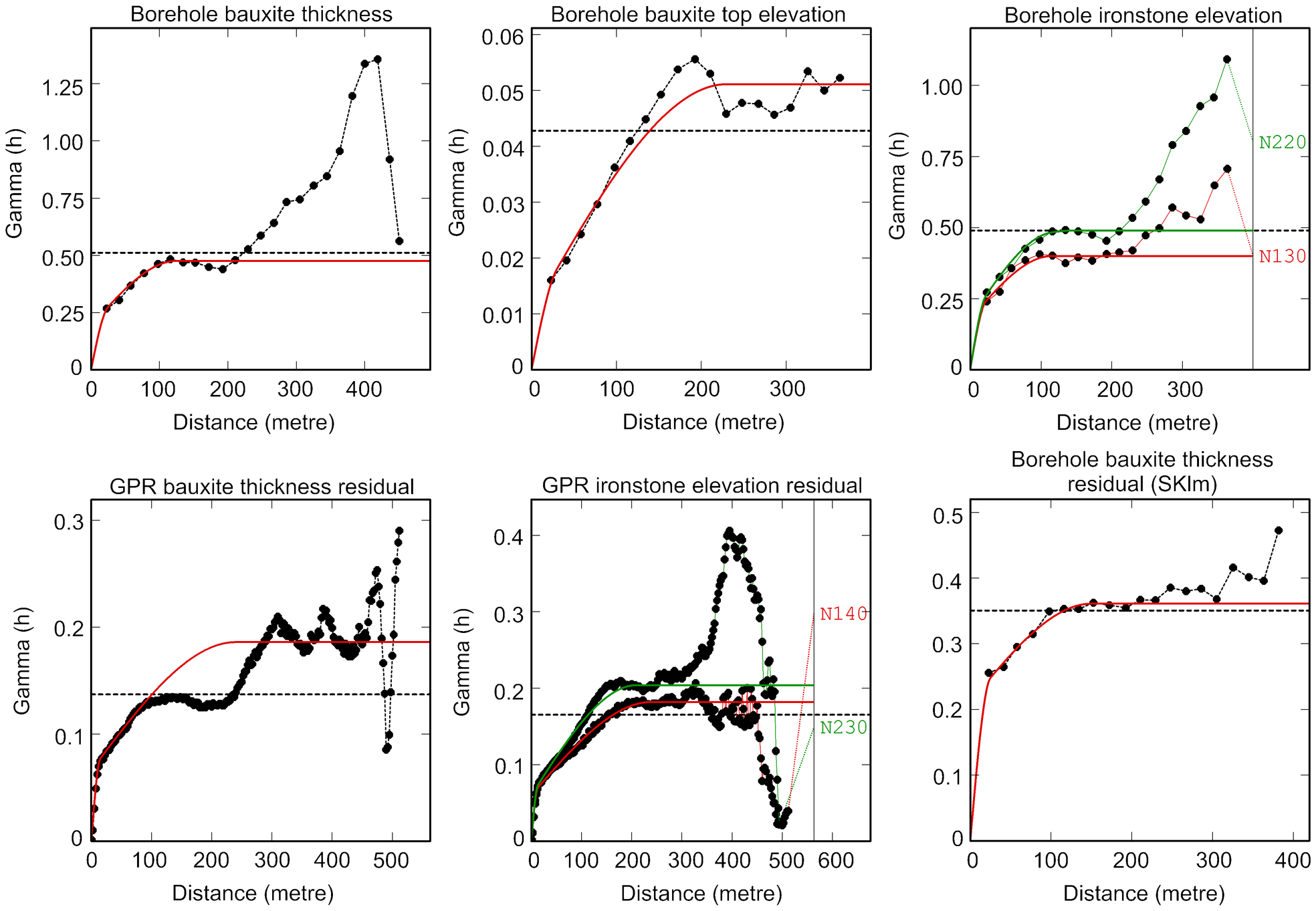
Directional semi-variograms and fitted mathematical models for the PC borehole and GPR data variables

To generate estimates for unsampled locations, the semi-variograms must be fitted with continuous functions to obtain semi-variances for any possible lag distances (Goovaerts, 1999). The spherical model with nested structures was used to model the semi-variograms of the PC borehole and GPR residual data variables. The semi-variograms of the PC borehole and GPR residual data variables and the mathematical models fitted to these semi-variograms are presented in Fig. 5.

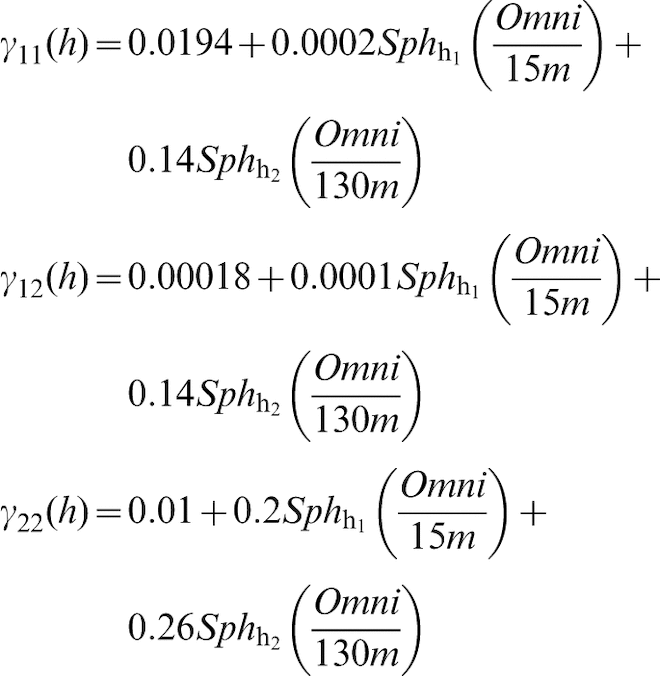
The model parameters of the semi-variograms shown in Fig. 5 are written as follows:

Borehole Bauxite thickness: (16)

Borehole bauxite top elevation: (17)

Borehole ironstone elevation: (18)

GPR bauxite thickness residual: (19)

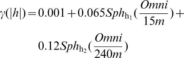
GPR ironstone elevation: (20)

SKLM bauxite thickness: (21)

Of the geostatistical prediction techniques, the OCCK requires the cross-semi-variogram to be used as a structural input in the kriging system (Rivoirard, 2001). To compute the cross-semi-variogram, there must be common locations at which both borehole and GPR data are available. The exploration borehole and GPR data values at co-located locations were first used to verify the linear relationship between the GPR and the exploration borehole data variables. The scatter plots presented in Fig. 6 exhibit reasonable correlations between exploration borehole bauxite thickness data and corresponding GPR bauxite thickness data, with a correlation coefficient (r) of 0·74, and between exploration borehole ironstone elevation data and corresponding GPR ironstone elevation data, with a correlation coefficient (r) of 0·61. The major reason for the low linear correlation between GPR and borehole data is due mainly to the shallowness of the bauxite/ironstone interface. The GPR equipment inherently cannot resolve the geological sections that are at very shallow elevations.

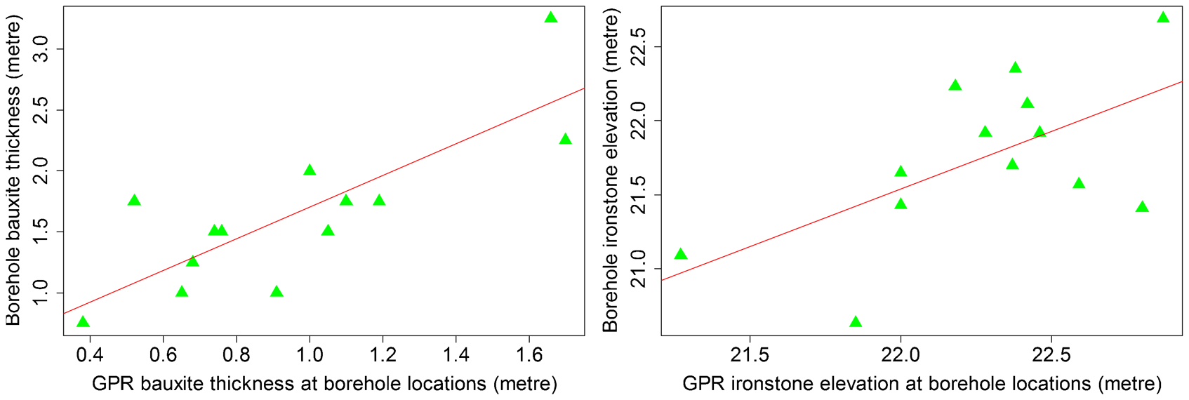
Linear correlation between exploration borehole and GPR data at co-located locations

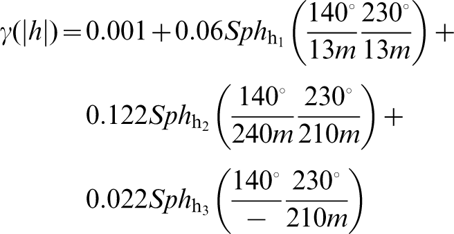
In the geostatistical framework, multivariate geostatistical prediction techniques require a stationary RF model for spatial prediction. As the cross-semi-variogram of the PC borehole and the GPR ironstone elevation variables exhibit non-stationarity, it is not possible to fit a linear model of coregionalisation (LMC) (Wackernagel et al., 1989) to the cross-semi-variogram of these variables. However, to achieve the objective of this case study, which is to predict the lateral variability of the bauxite/ironstone interface, an indirect prediction approach was used. That is, a bivariate prediction of exploration borehole bauxite thickness was first performed by OCCK, using a cross-semi-variogram fitted with an LMC. The OCCK exploration borehole bauxite thickness estimates were then subtracted from the OK exploration borehole bauxite top estimates to obtain indirect OCCK estimates of the exploration borehole ironstone elevation variable. For the sake of consistency, the indirect prediction approach was used for other prediction techniques as well. The auto- and cross-semi-variograms of the PC borehole bauxite thickness and GPR bauxite thickness variables were modelled by the same spherical structures to apply an LMC to the OCCK method, as presented in Fig. 7.

Auto- and cross-semi-variograms of the PC borehole and GPR bauxite thickness data fitted using an LMC with spherical structures

The LMC fitted to the auto- and cross-semi-variograms shown in Fig. 7 is written as follows (22) where γ₁₁(h) is the semi-variogram model of the PC borehole bauxite thickness variable, γ₁₂(h) is the cross-semi-variogram model of the PC borehole bauxite thickness and GPR bauxite thickness variables, and γ₂₂(h) is the semi-variogram model of the GPR bauxite thickness variable.

Prediction of surfaces

The prediction of surfaces was carried out in three stages: (1) defining the prediction grid, (2) defining the neighbourhood and (3) implementing the prediction algorithm. A 2D grid was defined with the following parameters: the origin was located at X = 3,256·6 m and Y = 20 078·7 m, the dimensions of the mesh were dx = 2·38 m and dy = 2·38 m, and the numbers of meshes were nx = 100 and ny = 225, which resulted in 22 500 meshes covering the entire area. Given the sampling grid of the GPR survey, the selected mesh dimensions were judged to be appropriate. A 2D polygon was used to delineate the boundary of the area, such that the extrapolation can be minimised. The number of meshes falling within the polygon area is 16 126. ISATIS software was used for performing the univariate and multivariate predictions. Considering the univariate prediction, the OK approach was first used with a unique neighbourhood to predict the spatial variability of the exploration borehole bauxite top elevation and ironstone elevation variables with semi-variogram models given in equations (17) and (18). The PC borehole data were also used with a moving neighbourhood, where the major range of the ellipse is 130 m and minor range is 100 m, to predict the ironstone elevation variability throughout the Kumbur mine area. The estimation maps representing the ironstone elevation variability both from exploration borehole and PC borehole data, as well as corresponding estimation variances, are presented in Fig. 8. It follows from the estimation maps presented in Fig. 8 that the drilling grid of exploration boreholes is too sparse to generate realistic predictions for ironstone elevation variability. It is therefore imperative that the dense geophysical data be incorporated in the prediction to improve the accuracy of the overall estimates.

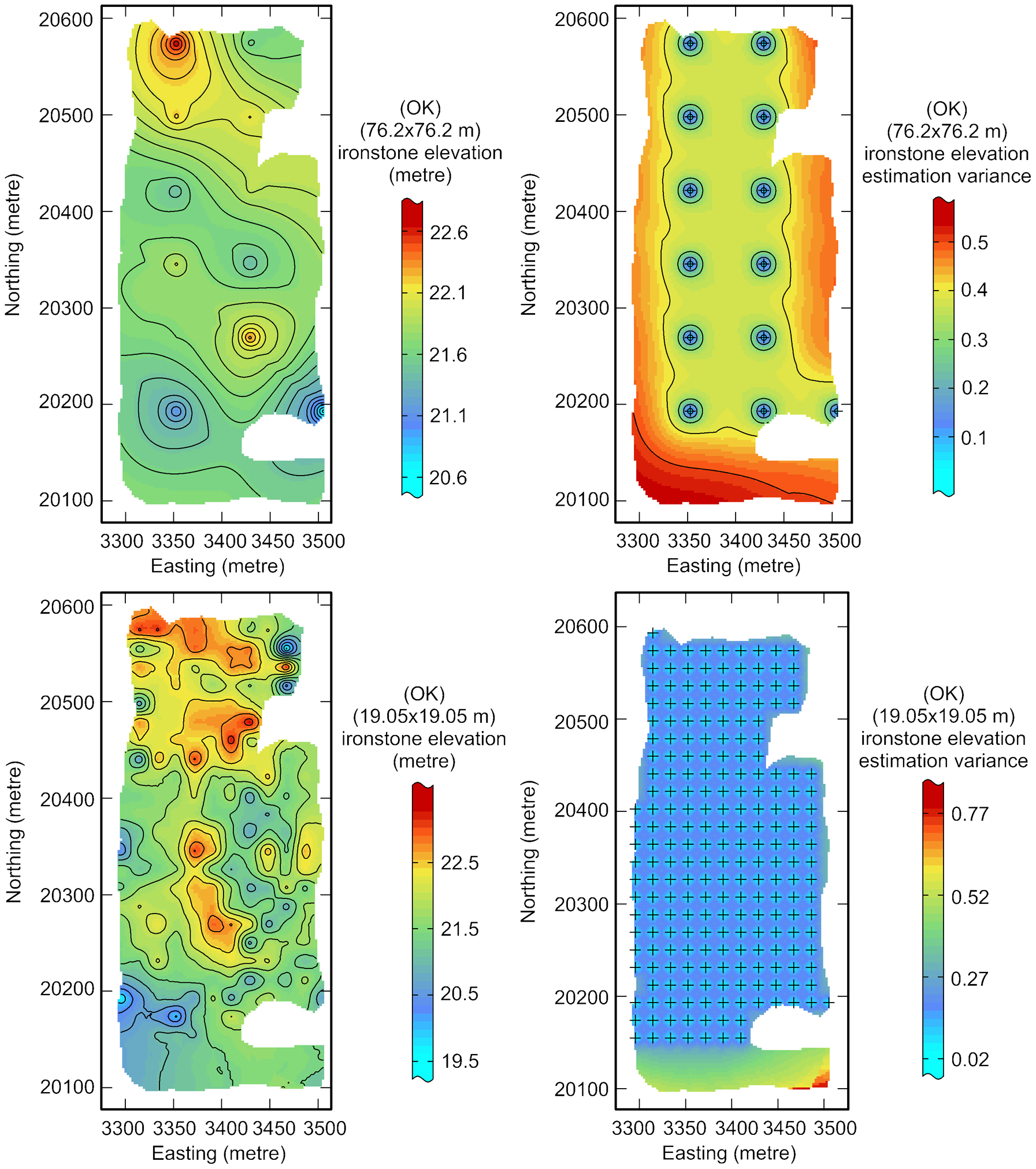
Maps of the borehole ironstone elevation from exploration (76·2×76·2 m) and production (19·05×19·05 m) borehole data and corresponding estimation variance

Considering the bivariate prediction of the ironstone elevation variability, the GPR ironstone elevation and GPR bauxite thickness variables should first be exhaustively sampled. That is, there must be a GPR datum at every estimation grid node and at every primary variable datum location. Hence, the GPR bauxite thickness residual and GPR ironstone elevation residual variables were predicted at the grid nodes using OK with the zero-mean and the semi-variogram models given in equations (19) and (20). The moving neighbourhood was used in the prediction. Because the GPR data are very dense and not as regular as the borehole data, 12 angular sectors were used to ensure that the neighbouring information could be evenly distributed around a target point. To avoid statistical instabilities, two samples were used for each angular sector. As a result, 24 points were selected within a search ellipse specified by the ranges given in equations (19) and (20). The trends represented by linear models were then added back to the residual estimates to obtain final GPR bauxite thickness and GPR ironstone elevation estimates.

Because the GPR bauxite thickness variable has been exhaustively sampled over the area, the SLR approach was first used to simply predict the borehole bauxite thickness at each grid node. The linear relation between the borehole bauxite thickness z(u_α) and the co-located GPR bauxite thickness y(u_α) data were modelled as z(u) = 0·413+1·338y(u), which leads to maps of borehole bauxite thickness and corresponding estimation variance. The SLR bauxite thickness estimates were subtracted from the OK bauxite top estimates to indirectly yield the SLR ironstone elevation estimates, as illustrated in Fig. 9. Given the SKLM approach, the bauxite thickness regression residuals were interpolated using SK with unique neighbourhoods. The estimated local means were then added back to the SK residual estimates to generate the final SKLM bauxite thickness estimates. These estimates were then subtracted from the OK bauxite top elevation to yield indirect ironstone elevation estimates. The corresponding estimation variance was calculated by adding estimation variance of OK bauxite top elevation to the estimation variance of SKLM bauxite thickness, as shown in the maps in Fig. 9. The OCCK approach was also used to predict the borehole bauxite thickness variable at the grid nodes using the cross-semi-variogram model given in equation (22). Because of the limited number of exploration borehole data points, the unique neighbourhood was selected for the prediction. The final indirect OCCK borehole ironstone elevation estimates were then derived by subtracting the OCCK borehole bauxite thickness estimates from the OK borehole bauxite top elevation estimates. The maps of OCCK ironstone elevation estimates and the corresponding estimation variance maps are illustrated in Fig. 9. Finally, the BAY approach was used to incorporate the densely sampled GPR data into the prediction of the ironstone elevation variability within the Kumbur mine area. Because of the BAY algorithm, the prior and likelihood distributions of the bauxite thickness variable were assumed to be Gaussian. The likelihood distribution of the bauxite thickness variable was predicted by the regression bauxite thickness estimate and corresponding regression variance. The prior distribution of the bauxite thickness was generated from the OK bauxite thickness estimate and corresponding estimation variance. The combination of prior and likelihood distributions of the bauxite thickness variable yielded the updated bauxite thickness distribution. As with other prediction techniques, the final BAY ironstone elevation estimates were generated by subtracting the BAY bauxite thickness estimates from the OK bauxite top elevation estimates, as presented in Fig. 9.

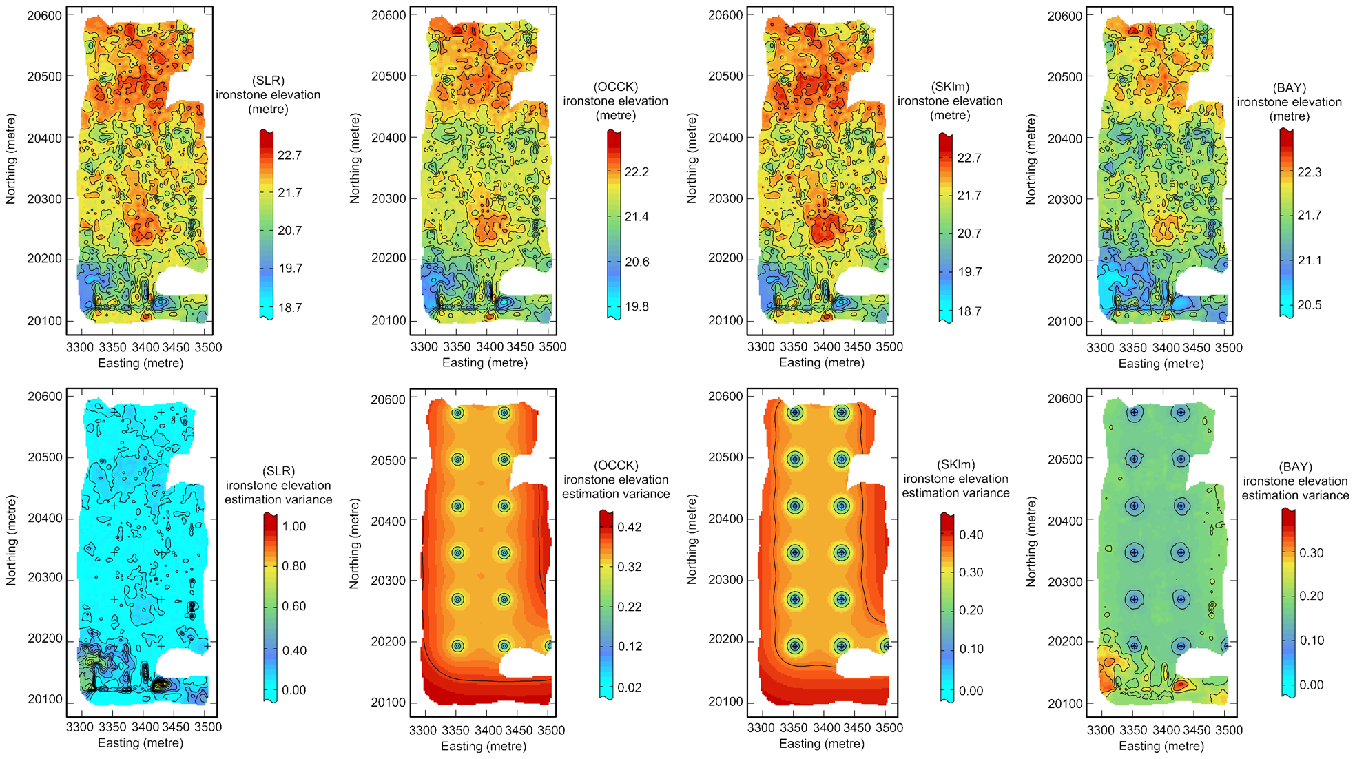
Maps of indirect ironstone elevation and corresponding estimation variance using BAY, SKLM, OCCK and SLR

Discussion and comparison of the different prediction algorithms

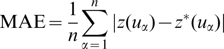
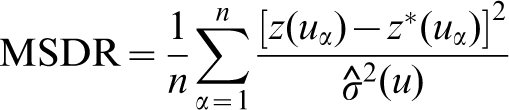
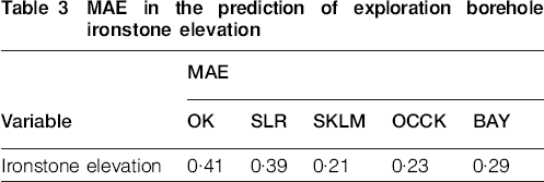
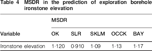
The performances of the four interpolators were assessed using a cross-validation procedure (Webster and Oliver, 2007). The accuracy of prediction is evaluated using the mean absolute error (MAE) and the mean squared deviation ratio (MSDR) criteria (23) (24) where n is the number of data values, z(u_α) is the true value, z*(u_α) is the estimated value, and is the estimation variance. If an algorithm is accurate, the MAE should be close to zero; if a semi-variogram is appropriate, the MSDR should be close to one. The borehole ironstone elevation values were re-estimated using the four prediction algorithms including SLR, SKLM, OCCK and BAY. As expected, the OK approach, which uses primary data only, yielded the highest MAE. The SLR approach, in which the MAE was calculated as the average residual value for the linear model fitted using 13 exploration borehole bauxite thickness values, yielded high MAE values due mainly to the reasonable correlation between exploration borehole bauxite thickness and corresponding GPR bauxite thickness variables. However, as the SLR estimates do not necessarily honour the data values at known locations, these estimates do not represent reality. Among the other bivariate prediction techniques, SKLM yielded the best performance. It appeared that the OCCK approach outperformed BAY estimates, which is primarily observed because OCCK treats the secondary variable as a random variable in the kriging system. The values of MSDR, which are close to 1, also indicate that the mathematical models fitted to the semi-variograms are appropriate for spatial prediction. The cross-validation results are listed in Tables 3 and 4.

Table 3

MAE in the prediction of exploration borehole ironstone elevation

Variable	MAE
Variable	OK	SLR	SKLM	OCCK	BAY
Ironstone elevation	0·41	0·39	0·21	0·23	0·29

Table 4

MSDR in the prediction of exploration borehole ironstone elevation

Variable	MSDR
Variable	OK	SLR	SKLM	OCCK	BAY
Ironstone elevation	1·120	0·910	1·09	1·13	1·17

After the Kumbur mine area was mined out, the final mine floor was surveyed and the survey points were interpolated using the nearest neighbour (NN) algorithm. The NN approach was selected such that the actual mine floor could be represented without a smoothing effect. The digital terrain model (DTM) of the actual mine floor and survey points are shown in Fig. 10.

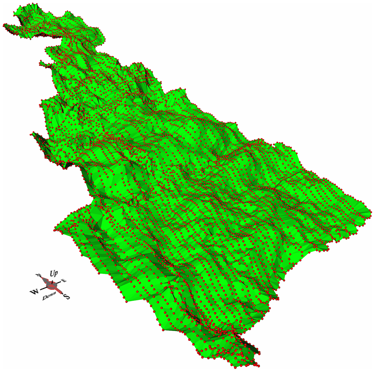
DTM representing the actual mine floor at the Kumbur mine area

As the survey points illustrated in Fig. 10 represent the front-end loader regions, the DTM of the actual mine floor does not necessarily honour the data at the borehole locations. However, the NN algorithm represents the actual mine floor without any smoothing effect, as presented in Fig. 10. The ironstone elevation surface predicted by the SKLM approach, as this approach yielded the smallest MAE values, was compared to the actual mine floor and the ironstone elevation surface predicted by the OK approach. The east–west and north–south cross-sections were taken along the borehole locations (northing 20 269·2 m and easting 3429 m), as presented in Figs. 11 and 12, respectively.

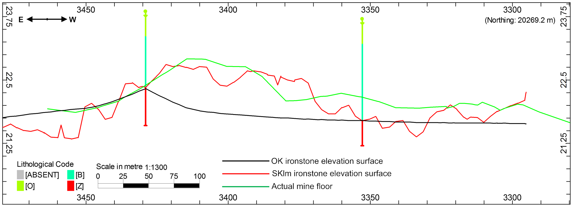
East–west cross-sections of the predicted ironstone elevation surfaces and the actual mine floor

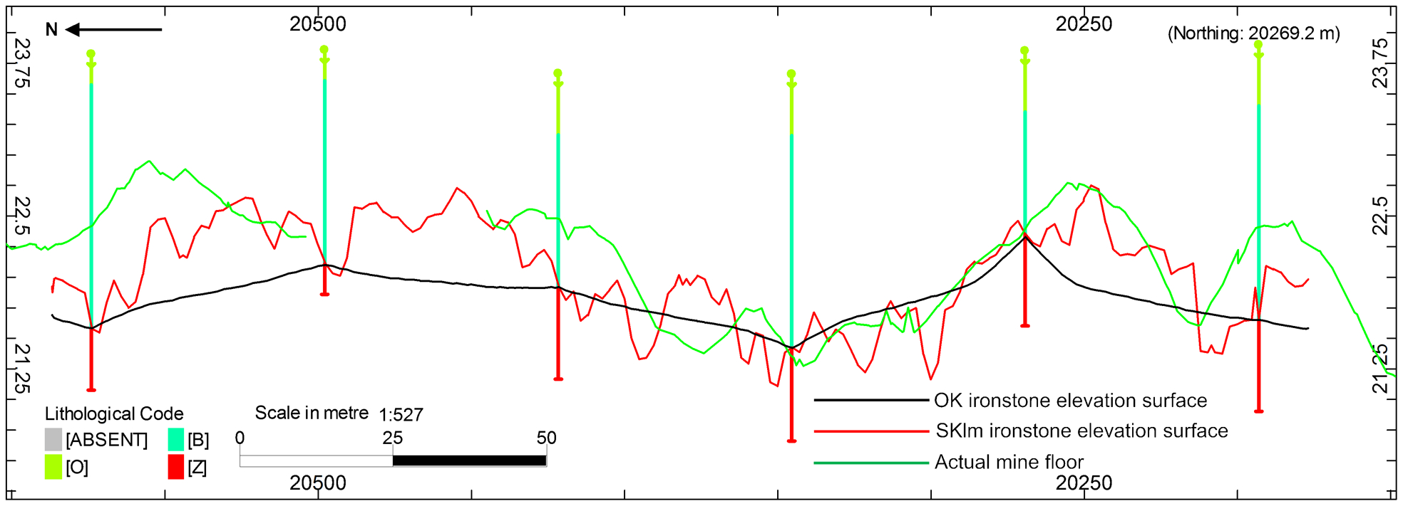
North–south cross-sections of the predicted ironstone elevation surfaces and the actual mine floor

The cross-sections shown in Figs. 11 and 12 clearly indicate that the bauxite/ironstone surface predicted by the SKLM approach exhibit a spatial pattern that is rather close to that of the actual mine floor. The SKLM estimates appeared to honour the known data at their locations, as the kriging is an exact interpolator. However, this does not apply to the surface representing the actual mine floor, which represents the front-end loader regions where known data are not necessarily honoured at their locations because of the mining equipment constraint. As it is clear from the cross-sections, the bauxite/ferricrete surface predicted by SKLM appears to be locally more variable than that of the actual mine floor. This is mainly because the large mining equipment (a front-end loader) cannot track the actual bauxite/ferricrete surface with high precision because of the mining equipment constraint. Therefore, for accurate grade control practice, it is suggested that the predicted bauxite/ferricrete interface be optimised such that the resulting surface will account for the mining equipment constraint-induced dilution and ore loss. The aforementioned cross-sections also confirm that there is a large difference between the bauxite/ironstone surfaces predicted by the OK and SKLM approaches. This result clearly indicates why the bauxite ore loss and ironstone dilution occurring at the time of mining cannot be quantified when the bauxite/ironstone surface predicted by the OK approach was used to geologically constrain the block model.

Conclusion

Geostatistics allows one to incorporate the densely sampled secondary information into the prediction of the spatial variability of a sparsely sampled primary variable within a given domain. In this case study, four prediction algorithms, including SKLM, SLR, OCCK and BAY, were used to incorporate exhaustive GPR data into the mapping of lateral variability of the bauxite horizon within the laterite-type bauxite deposit at Weipa in northern Queensland, Australia. Of the prediction techniques, the SLR is the most straightforward approach that derives borehole ironstone elevation values from the co-located GPR ironstone elevation data. The major drawback of this approach is that it does not account for sample values surrounding an unknown value, which leads to the fact that the known values are not necessarily honoured at their locations. The SKLM approach allows one to account for the exhaustive GPR data by interpolating the regression residuals. The local means were later added to the SK regression residual estimates to yield the final SKLM ironstone elevation estimates. Considering the OCCK approach, the secondary variable is treated as a random variable with an expected value and a semi-variogram. In comparison to other prediction algorithms, the OCCK approach is more demanding, as three semi-variograms need to be modelled jointly. As for the BAY approach, the dense GPR data were incorporated into the prediction of the bauxite/ironstone interface by combining the prior and likelihood distributions of the bauxite thickness variable. In the BAY approach, the prior and likelihood distributions were assumed to be Gaussian. The north–south and east–west cross-sections taken along the borehole locations indicate that the SKLM borehole ironstone elevation estimates are highly correlated with the actual mine floor.

This case study shows that incorporating the exhaustively sampled GPR data has led to estimates that correspond closely with the actual mine floor. This improvement becomes obvious when compared with the OK estimates, which were obtained solely from the borehole data. It is apparent that the OK estimates represent a surface with excessive smoothness and is inconsistent with the actual mine floor.

Footnotes

Acknowledgements

The work reported in this paper was funded by Rio Tinto Alcan, Australia. The authors thank Jan Francke, Michael Mills and Glenn White for their advice and support.

References

Abzalov

and Bower

2009. Optimisation of drill grid at the Weipa bauxite deposit using conditional simulation, 7th International Mining Geology Conference, The Australasian Institute of Mining and Metallurgy, Melbourne, 247–252.

Ahmed

and De Marsily

1987. Comparison of geostatistical methods for estimating transmissivity using data on transmissivity and specific capacity, Water Resour. Res., 23, (9), 1717–1737.

ASTM D 5923–96. 2004. Standard guide for selection of Kriging methods in geostatistical site investigation, 443–446, USA, International ASTM.

ASTM D 6432–99. 2005. Standard guide for using the surface ground penetrating radar method for subsurface investigation, 984–1000, West Conshohocken, PA, ASTM International.

Baker

, Jordan

and Pardy

2007. An introduction to ground penetrating radar (GPR), in Stratigraphic analysis using GPR, (eds. Baker

GS.

and Jol

H M

), 1–18, Geological Society of America.

Bardossy

, Bogardi

and Kelly

. 1986. Geostatistical analysis of geoelectric estimates for specific capacity, J. Hydrol., 84, (1–2), 81–95.

Bardossy

and Aleva

GJJ

. 1990. Lateritic bauxites, Amsterdam, Oxford, New York, Tokyo, Elsevier.

Barsottelli-Botelho

and Luiz

. 2011. Using GPR to detect bauxite horizons in laterite deposits of Amazon Basin, Brazil, 73rd European Association of Geoscientists and Engineers, Vienna, Austria.

Bourennane

and King

2003. Using multiple external drifts to estimate a soil variable, Geoderma, 114, 1–18.

10.

Campbell

1994. Geophysical contribution to mine development planning-a risk reduction approach, 15th CMMI Congress, (ed. C. R. Anhaeusser), Johannesburg, The Southern African Institute of Mining and Metallurgy, 283–325.

11.

Chihi

, Galli

, Ravenne

, Tesson

and de Marsily

2000. Estimating the depth of stratigraphic units from marine seismic profiles using nonstationary geostatistics, Nat. Resour. Res., 9, (1), 77–95.

12.

Chiles

and Delfiner

1999. Geostatistics modelling spatial uncertainty, New York, John Wiley & Sons.

13.

Cressie

1993. Statistics for spatial data, New York, Wiley.

14.

Davis

. 2002. Statistics and data analysis in geology, New York, Chichester, Brisbane, Toronto, Singapore, Wiley.

15.

Davis

and Annan

. 1989. Ground-penetrating radar for high-resolution mapping of soil and rock stratigraphy, Geol. Prospect., 37, 531–551.

16.

Dowd

. 1997. Geostatistical characterisation of three-dimensional spatial heterogeneity of rock properties at Sellafield, Trans. Inst. Min. Metall., Sect. A, 106, 133–147.

17.

Dowd

and Pardo-Iguzquiza

2006. Core-log integration: optimal geostatistical signal reconstruction from secondary information, Trans. Inst. Min. Metall. B, 115, (2), 59–70.

18.

Doyen

. 1988. Porosity from seismic data: a geostatistical approach, Geophysics, 53, (10), 1263–1275.

19.

Doyen

, den Boer

and Pillet

. 1996. Seismic porosity mapping in the Ekofisk field using a new form of collocated cokriging, Soc. Pet. Eng., 36498, 21–30.

20.

Eggleton

. 2001. The regolith glossary, Surficial geology, soils and landscapes, Canberra, Cooperative Research Centre for Landscape Evolution and Mineral Exploration.

21.

Eggleton

and Taylor

1998. Selected thoughts on ‘laterite’, New Approaches to an Old Continent, 3rd Australian Regolith Conference, Kalgoorlie, Co-operative Research Centre for Landscape Evolution and Mineral Exploration, Perth, (eds. Taylor

and Pain

), 209–226.

22.

Eggleton

and Taylor

2005. Bioturbation of the Weipa bauxite, in Regolith 2005-ten years of CRC LEME, (ed. Roach

I C

), CRC-LEME, 83–85.

23.

Erten

2012. Profiling and mining control to mitigate dilution effect from SiO₂ at the base of a bauxite deposit, Doctor of Philosophy, The University of Queensland, Brisbane.

24.

Erten

, Kizil

, Topal

and McAndrew

2013. Spatial prediction of lateral variability of a laterite-type bauxite horizon using ancillary Ground-penetrating radar data, Nat. Resour. Res., 22, (3), 207–227.

25.

Evans

. 1965. Bauxite deposits at Weipa. Geology of Australian Ore Deposits, 8th Commonwealth Mining and Metallurgical Congress. Australia and New Zealand, The Australasian Institute of Mining and Metallurgy, Melbourne, (ed. McAndrew

), 396–401.

26.

Evans

. 1975. Weipa deposit, Queensland, in Economic geology of Australia and New Guinea, (ed. Knight

C L

), 959–964, Melbourne, Australasian Institute of Mining and Metallurgy.

27.

Fallon

, Fullagar

and Sheard

. 1997. Application of geophysics in metalliferous mines, Aust. J. Earth Sci. Int. Geosci. J. Geol. Soc. Aust., 44, (4), 391–409.

28.

Francke

. 2012a. A review of selected ground penetrating radar applications to mineral resource evaluations, J. Appl. Geophys., 81, 29–37.

29.

Francke

. 2012b. The role of ground penetrating radar in bauxite resource evaluations, 14th International Conference on Ground Penetrating Radar (GPR), Shanghai, China, IEEE Geoscience and Remote Sensing Society, 459–463.

30.

Francke

and Nobes

. 2000. A preliminary evaluation of GPR for nickel laterite exploration, Proc. 8th Int. Conf. on Ground Penetrating Radar, Gold Coast, Queensland, (eds. Noon

D A

, Stickley

G F

and Longstaff

), SPIE-International Society for Optical Engine, 7–12.

31.

Francke

and Parkinson

2000. The new role of geophysics in nickel laterite exploitation and development, Toronto, Canada, Mining Millennium/PDAC Convention.

32.

Francke

and Utsi

2009. Advances in long-range GPR systems and their applications to mineral exploration, geotechnical and static correction problems, First Break, 27, 85–93.

33.

Goovaerts

1997. Geostatistics for natural resource evaluation, New York, Oxford University Press.

34.

Goovaerts

1999. Geostatistics in soil science: state-of-the-art and perspectives, Geoderma, 89, 1–45.

35.

Goovaerts

2000. Geostatistical approaches for incorporating elevation into the spatial interpolation of rainfall, J. Hydrol., 228, 113–129.

36.

Goovaerts

and Kerry

2010. Using ancillary data to improve prediction of soil and crop attributes in prediction agriculture, in Geostatistical applications for precision agriculture, (ed. Oliver

M A

), 167–193, New York, Springer.

37.

Isaaks

and Srivastava

. 1989. An introduction to applied geostatistics, New York, Oxford University Press.

38.

Isbell

. 1983. Kimberley-Arnhem-Cape York (III), in Soils: an Australian viewpoint. CSIRO division of soils, Melbourne and Academic Press London, CSIRO, 189–199.

39.

Journel

and Huijbregts

. 1978. Mining geostatistics, London, Academic Press.

40.

Journel

, Kyriakidis

and Mao

2000. Correcting the smoothing effect of estimators: a spectral postprocessor, Math. Geol., 32, (7), 787–813.

41.

Kay

and Dimitrakopoulos

2000. Integrated interpolation methods for geophysical data: applications to mineral exploration, Nat. Resour. Res., 9, (1), 53–63.

42.

Keary

and Brooks

1994. An introduction to geophysical exploration, 2nd edn, Oxford, Blackwell Scientific Publications.

43.

Loughnan

and Bayliss

1961. The mineralogy of the bauxite deposits near Weipa, Queensland, Am. Mineral., 46, 209–217.

44.

Matheron

1963. Principles of geostatistics, Econ. Geol., 58, 1246–1266.

45.

Matheron

1971. The theory of regionalised variables and its applications, Cahiers Cent. Morph. Mat., 5, 211.

46.

McDonald

and Mandla

1993. Bauxite mining and beneficiation by Comalco Aluminium Ltd at Weipa, Old, Aust. Min. Metall. Monogr., 19, 750–753.

47.

McKenzie

, Jacquier

, Isbell

and Brown

2004. Australian soils and landscapes: an illustrated compendium, Melbourne, CSIRO.

48.

Morgan

. 1996. The geology of the Comalco bauxite resource: a beginner's guide, Comalco Mineral and Alumina Report WTR 96/10.

49.

Morgan

. 1992a. Geology of the spheres at Weipa, 7th International Congress of Icsoba, Icsoba, Balatonalmadi, Hungary, Acad. Yougoslave des Sciences et des Arts, 61–74.

50.

Morgan

1992b. Bauxite geological modelling system, Weipa, Comalco Minerals and Alumina.

51.

Morgan

1993. Methods for improving the control of the bauxite mine floor and their impact on reserve tonnage and grade, Weipa, Comalco Minerals and Alumina.

52.

Morgan

1995. An investigation into the application of ground penetrating radar to the weipa mining operation, Weipa, Comalco Minerals and Alumina.

53.

Myers

. 1989. To be or not to be … stationary? That is the question, Math. Geol., 21, (3), 343–362.

54.

Odeh

IOA

, McBratney

and Chittleborough

. 1995. Further results on prediction of soil properties from terrain attributes: heterotopic cokriging and regression-kriging, Geoderma, 67, 215–226.

55.

Pardo-Iguzquiza

and Dowd

. 1998. The second-order stationary universal Kriging model revisited, Math. Geol., 30, (4), 347–377.

56.

Rivoirard

2001. Which models for collocated cokriging? Math. Geol., 33, (2), 117–131.

57.

Schaap

. 1990. Weipa kaolin and bauxite deposits, in Geology of the mineral deposits of Australia and Papua New Guinea, (ed. Hughes

F E

), 1669–1673, The Australasian Institute of Mining and Metallurgy.

58.

Singh

. 2007. Ground penetrating radar (GPR) ‘mineral base profiling and orebody optimisation’. The 6th International Heavy Minerals Conference ‘Back to Basics’. The Southern African Institute of Mining and Metallurgy, Hluhluwe, South Africa, 179–182.

59.

Taylor

and Eggleton

2004. ‘Little Balls’ The origin of the Weipa bauxite, in Regolith 2004, (ed. Roach

I C

), Caberran, CRC LEME, 350–354.

60.

Taylor

, Eggleton

, Foster

and Morgan

. 2008a. Landscapes and regolith of Weipa, northern Australia, Aust. J. Earth Sci., 55, 3–16.

61.

Taylor

, Eggleton

, Foster

, Tilley

, Gleuher

and Morgan

. 2008b. Nature of the Weipa bauxite deposit, northern Australia, Aust. J. Earth Sci., 55, 45–70.

62.

Wackernagel

2002. Multivariate geostatistics, Berlin, Springer.

63.

Wackernagel

, Petitgas

and Touffait

1989. Overview of methods for coregionalisation analysis, in Geostatistics, (ed. M. Armstrong), 409–420, Dordrecht, Kluwer Academic Publishers.

64.

Watts

1997. Exploring for nickel in the 90s, or ‘Til depth us do part’. Exploration 97: Fourth Decennial International Conference on Mineral Exploration, Toronto, Canada.

65.

Webster

and Oliver

. 2007. Geostatistics for environmental scientists, England, John Wiley & Sons, Ltd.

66.

, Tran

, Srivastava

and Journel

. 1992. Integrating seismic data in reservoir modelling: the collocated cokriging alternative, 67th Annual Technical Conference and Exhibition, Society of Petroleum Engineers, Washington, DC.

67.

Yamamoto

. 2008. Estimation or simulation? That is the question, Comput. Geosci., 12, 573–591.