Three-dimensional numerical modelling of discontinuous fibre composite architectures

Abstract

A three-dimensional geometrical model is presented for generating discontinuous random fibre architectures consisting of high filament count bundles. The fibre network model randomly distributes fibre bundles in a three-dimensional volume using a non-contact algorithm, together with Catmull–Rom spline interpolation, to provide a physically representative material. Only the spines of the fibre bundles are modelled, using truss elements to permit high fibre volume fractions of up to 60%, with no restriction on the fibre bundle aspect ratio. ABAQUS/Standard is used to predict the tensile performance for coupons with varying levels of out-of-plane fibre curvature. The effect of fibre curvature was found to be insignificant for tensile modulus, but a 34% reduction in ultimate tensile strength (UTS) was observed when adjusting the maximum permissible out-of-plane angle of fibres from 1 to 35°. A novel method for characterising the degree of out-of-plane fibre curvature within experimental test coupons is also discussed.

Keywords

Discontinuous Modelling Random Finite element Carbon fibre

Introduction

Background

Discontinuous, long fibre composites constitute a large proportion of fibre reinforced materials used in automotive and marine applications due to their versatility and relatively low manufacturing costs.1 Consequently, a number of automated discontinuous deposition processes have become available, enabling fibre architectures to be tailored with varying fibre length, bundle size, alignment and fibre volume fraction. 2 , 3 Such advancements have reduced the performance gap between discontinuous and continuous materials, making these materials more suitable for structural applications. Typical materials used for high performance applications include advanced structural moulding compounds4^–6 and directed carbon fibre preformed (DCFP) materials. 2 3 2,3,7 Accurate characterisation of these architectures, however, still remains a challenge due to the stochastic nature of the fibre architecture and the compounding effects of the aforementioned parameters. While discontinuous fibre materials offer greater levels of design flexibility compared with conventional metallics and continuous fibre composites, the ‘complex’ nature of the material and the high levels of variability have prevented wider commercialisation.

Accurate prediction of the mechanical performance is essential if these materials are to be adopted for structural applications in order to reduce costly experimental testing programmes and to facilitate design optimisation. While textile fabrics have a repeatable geometry and can be modelled as a relatively small periodic unit cell, the discontinuous fibre composites are highly heterogeneous and are non-repeating. A much larger geometric entity is required to capture this material heterogeneity, and is described as being a representative volume element (RVE). Definitions of RVEs differ, but in the context of this paper, it is established as being a volume which is sufficiently large enough to contain a large number of inclusions in a heterogeneous material, and the effective properties derived from the RVE represent the true material properties in macroscopic scale.8 The RVE size can be an order of magnitude greater than a periodic unit cell, and the challenge, therefore, is to analyse sufficiently large volumes while remaining computationally inexpensive. This inevitably leads to numerous modelling approaches for characterising the material, which have their own respective assumptions or simplifications, as discussed below.

Existing numerical models

Creating models with a suitable fibre volume fraction V_F, or ‘fibre packing’, is the main limiting factor when generating numerical RVEs for fully random fibre architectures. Random sequential adsorption (RSA) schemes are typically used to add successive fibres to the RVE, avoiding fibre–fibre intersection by discarding physically contacting fibres. ‘Jamming’ is experienced when the pockets of free space are too small to accept any additional fibres. Consequently, high fibre volume fractions are not achievable. In addition, this approach effectively homogenises the material and does not reflect the localised areas of high and low volume fractions often observed in automated deposition processes. The RSA technique produces architectures that appear random on a global scale, but clusters of aligned fibres are introduced at the local level.9 This is particularly a problem for structural materials, which typically feature high fibre volume fractions approaching 55%7 and bundle length/width aspect ratios (ARs) of up to 10.

Evans and Ferrar9 demonstrated that the achievable fibre volume fraction with RSA techniques is a function of the fibre AR. Volume fractions as high as 60% can be achieved for ARs of 1 (sphere), but this reduces to <40% for ARs of 6. Kari10 studied the influence of fibre waviness in discontinuous fibres and created RVEs with inclusions of different ARs to achieve higher fibre volume fractions. Pan et al.11 recently developed a modified RSA technique to model ARs of up to 20. RVEs are discretised into mats, which consist of two plies, and fibres move between plies at local intersection points. The underlying problems of an RSA scheme are still evident, and each layer eventually becomes homogenised. While some out-of-plane fibre curvature is captured, the maximum achievable V_F is still limited to 35%. The fibre is also only permitted to move between plies and not between mats, limiting the accuracy of the model for out-of-plane property predictions.

Harper et al.12 developed a two-dimensional (2D) RVE model where the spine of each fibre bundle was modelled using one-dimensional (1D) beam elements. Bundles were limited to just axial material properties, with an effective circular cross-section. Two-dimensional resin elements, with a representative thickness, hosted the beams using the ABAQUS *Embedded Element technique. Fibre–fibre contacts were permitted, and consequently, there was no upper limit for V_F or fibre AR. The tensile predictions were found to be within 10 and 20% for stiffness and strength respectively for studies of varying volume fraction and length.7 The model was computationally inexpensive, enabling large volumes (200×200×3 mm) to be analysed, but simulations were limited to in-plane tension because of the 2D fibre architecture.

The model in Ref. 12 forms the foundation for the work presented in the current paper. The embedded element technique has been extended into three dimensions to account for out-of-plane fibre curvature effects. Pan et al. attempted to capture this in Ref. 11, but the linear segments used to model the fibres change orientation sharply, resulting in large local stress concentrations at the inflection points. This is not physically representative, as Fig. 1 indicates that the fibres undulate gradually without abruptly changing direction.

Figure 1

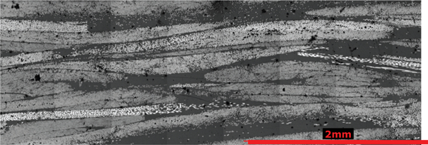
Micrograph of discontinuous carbon fibre composite manufactured by DCFP process: fibre length is 30 mm, and global fibre volume fraction is 50%

Model development

A versatile numerical modelling programme has been developed using the C# programming language. The model principally aims to characterise a number of mesoscale discontinuous fibrous materials, such as advanced structural moulding compounds, P4, DCFP and BRAC3D,2^–7 but can be expanded to receive data from process driven models, such as in Ref. 13. The three-dimensional (3D) fibre network consists of multiple fibre bundle spines with an effective cross-section, defined as a function of filament count and bundle V_F.

Generation of RVE cell and fibre coordinates

A similar approach to Ref. 12 has been adopted for generating the in-plane fibre coordinates. An RVE of width W×height H×thickness T is specified, together with a nominal fibre bundle length L and cell V_F. The centre of the mass of each fibre is assigned a random Cartesian coordinate (X, Y) in the range of 0⩽X⩽(W+2L) and 0⩽Y⩽(H+2L), which represents a secondary boundary outside of the RVE cell to ensure that the edge effects of the fibre are captured within the RVE. The fibres are assigned a random in-plane orientation Ø (0,2π), from which the fibre end coordinates are derived [(X₁, Y₁) and (X₂, Y₂)]. Each fibre is deposited sequentially within the outer cell and evaluated to see whether it lies within the boundaries of the RVE. If a fibre segment crosses the boundaries of the RVE, a Liang–Barsky cropping algorithm is employed to crop the fibre end coordinates to the RVE cell. The V_F is calculated cumulatively based on the cropped length of fibre segments within the RVE. The adsorption algorithm continues until the threshold V_F is reached.

Fibre intersection algorithm

The end coordinates of each cropped fibre end are successively passed to the intersection algorithm and initially assigned height values Z₁ and Z₂ equal to the radius of the fibre cross-section (D/2). Each subsequent fibre bundle is assessed to establish whether an intersection exists on the projected X–Y plane against previously deposited fibres. A straight line is returned if no intersections exist. In the case of an intersection at point (X_i, Y_i), the height of the intersected fibre Z_i is calculated, and a new control point (X_i, Y_i, Z_i+D) is created for the newly deposited fibre. Once all the intersection points for a fibre have been detected and computed, the end points and the intersection control points (X_i−n, Y_i−n, Z_i−n) are passed into a Catmull–Rom algorithm,14 and a smooth cubic curve is returned.

Catmull–Rom spline interpolation was chosen due to its local control and C¹ continuity (the derivative of the curve is always continuous). Such features ensure that the curve passes through the control points and the C¹ continuity maintains a continuous curve tangent along the fibre length, avoiding local sharp changes in the out-of-plane gradient, as in Ref. 11. The algorithm is also one of the least computationally expensive methods, requiring the minimum number of control points to approximate a curve.

Given four control points, P0–P3 (Fig. 2), a spline is generated between points P1 and P2 based on the tangents created from the end points, P0–P3 inclusive. The tangent to the curve at P1 is parallel to the chord between P0 and P2, and the tangent at P2 is parallel to the chord between P1 and P3. The number of interpolation points between control points is calculated based on the fibre element size for the finite element (FE) analysis. Several curvature tolerances have been incorporated to regulate the fibre architecture. A consolidation step is used to combine control points in high concentration areas based on a minimum spline length S_min specified by the user. Similarly, a maximum spline length S_max is set to ensure that long linear fibre segments are not generated. Finally, the maximum out-of-plane angle between two control points (Fig. 3) can be specified with respect to the X–Y plane to regulate the level of curvature.

Figure 2

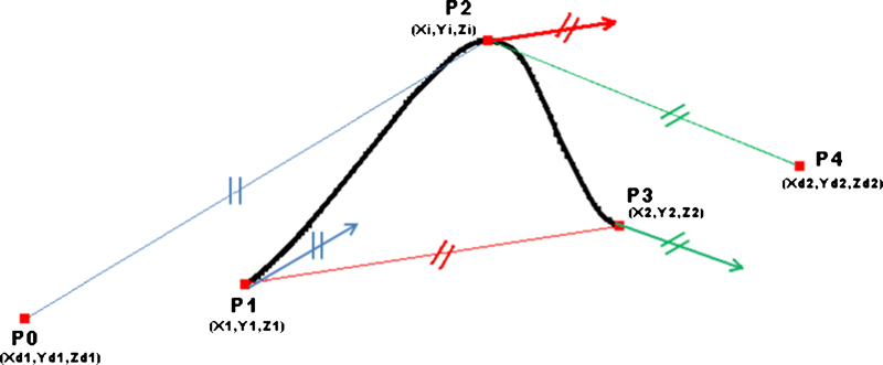
Schematic of Catmull–Rom cubic spline method: P0–P4 are control points

Figure 3

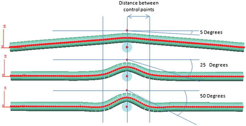
Effects of maximum out-of-plane angle between control points (top: 5°; middle: 25°; bottom: 50°): red dots represent interpolation points, and distance between each point represents beam element length

Fibre compaction algorithm

Fibres initially fall to the A surface of the mould tool as they are deposited, and the fibre architecture is built from the ‘bottom-up’. While this is useful for characterising levels of preform loft (Fig. 4) and the level of B surface waviness from a vacuum infusion part, it does not represent the fibre architecture achieved from closed mould processes. A reverse procedure of the intersection elevation algorithm has been developed, which is referred to as a ‘top–down’ approach. The fibre architecture is built from the top layer, with the last fibre, now the first. Intersection control points from both ‘bottom-up’ (X_i−n, Y_i−n, Z_i−n) and ‘top–down’ (X_i2−n, Y_i2−n, Z_i2−n) approaches are mirrored onto each fibre. The height values from each approach are then averaged [(Z_i+Z_i2)/2], and the control points are again passed into the Catmull–Rom algorithm to produce the final compressed fibre architecture of the cell, as shown in Fig. 5.

Figure 4

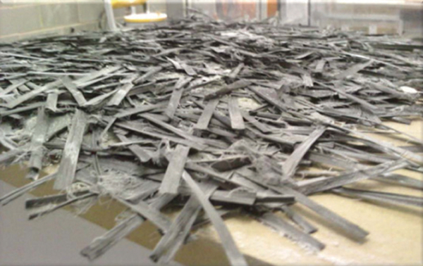
‘As deposited’ preform from typical automated preforming technique

Figure 5

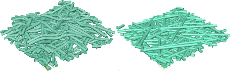
RVE of 30×30×3 mm at 40% fibre V_F, nominal fibre length of 36 mm and maximum out of plane curvature angle of 25° (left: uncompressed; right: compressed)

Finite element modelling

An ABAQUS/Standard input deck is generated by the programme, which contains the node and element definitions of the fibres and resin (Fig. 6). Reduced integration 20-node quadratic brick elements (C3D20R) are used to model the epoxy resin material in the FE analysis (FEA). Fibre bundles are represented using 1D quadratic truss elements (T3D3). The embedded element technique, a form of multipoint constraint in ABAQUS/Standard, is used to host the fibres in the matrix material. Truss elements are computationally inexpensive, allowing larger volumes of material to be studied when compared to shell or continuum elements. Convergence of the overall stress response of the RVE from a mesh sensitivity analysis indicated that 0·4 mm truss elements and 0·4×0·4×0·4 mm continuum elements should be used for subsequent simulations.

Figure 6

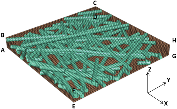
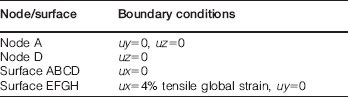
Numerical geometry imported into ABAQUS/CAE and rendered

The maximum principal stress failure criterion is used in a continuum damage approach to initiate failure in the models via a user defined material (UMAT), using state variables in ABAQUS/Standard to monitor damage progression. Full details of the UMAT stiffness degradation scheme are detailed in Ref. 7. The applied boundary conditions directly simulate an experimental tensile test. The node labels used to define the boundary conditions are presented in Fig. 6.

Node/surface	Boundary conditions
Node A	uy = 0, uz = 0
Node D	uz = 0
Surface ABCD	ux = 0
Surface EFGH	ux = 4% tensile global strain, uy = 0

A 12K T700 Toray 50C tow is used throughout the analyses, which has a 0·767 mm² cross-sectional area, assuming a circular cross-section with a 60% fibre volume fraction. The bundle properties were derived experimentally in Ref. 7. RVE cell sizes of 30×30×3 mm have been modelled in all cases with a nominal fibre length of 36 mm.

Results and discussion

RVE generation

Geometrical data generated from the programme have been imported into ABAQUS/CAE for visual comparison. Figure 5 (left) shows the fibre bundles before consolidation, reflecting the ‘as deposited’ state (Fig. 4) outlined in Refs. 2 and 7. Future developments will enable the uncompressed fibre architecture to be used for characterising preform loft as well as B surface waviness for vacuum infused parts. The level of fibre waviness is expected to be a function of in-plane fibre orientation, fibre length and bundle filament count. Figure 5 (right) depicts the fibre architecture after compaction from a matched tool process. Naturally, the extent of the fibre curvature decreases after the compaction step as the fibres become flattened.

While the representations of the cross-sections appear to be intersecting in Fig. 5 (right), the spines of the fibre remain spaced within the RVE. This anomaly occurs because a constant circular profile is currently swept along the fibre spines. No attempt has been made to implement local bundle volume fraction variations resulting from cross-sectional deformation at intersection points. Note also that the nature of the truss elements used in the subsequent FEA does not facilitate the assignment of different cross-sectional profiles and was chosen in the current study for its computational efficiency. No fibre jamming occurs, and there appears to be no restriction on the fibre volume fraction using the current modelling approach.

The model successfully allows the integration of fibre curvature and fibre crimp, providing smooth undulations of the fibres through the thickness, as shown in Fig. 1. The degree of fibre curvature is user controlled, enabling its effect on the macroscopic material properties to be considered in isolation. The actual level of out-of-plane curvature experienced in experimental coupons is currently unknown, due to difficulties in extracting and recreating large volumes of material from X-ray computer tomography (CT). Current work is focused on developing a method using a single 10 μm cobalt wire embedded at the centre of each fibre bundle. The metallic wire provides greater levels of contrast than the carbon fibres and epoxy matrix and can be easily distinguished in the image (Fig. 7). The cobalt wires are filtered within the X-ray, and nodes (control points) are placed along the fibre spines at intervals equivalent to those used in the FEA mesh. A number of curvature tolerances have been integrated into the model to enable experimental fibre architectures to be recreated from these control points.

Figure 7

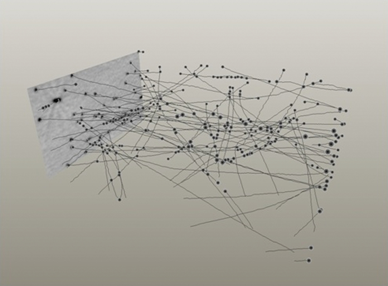
X-ray CT image of moulded specimen with cobalt wires embedded into fibre bundles: dark spheres represent example fibre control points (currently only at bundle ends), and rectangle indicates scan plane

Out-of-plane fibre curvature analysis

The effect of fibre curvature on the mechanical properties has been studied by controlling the maximum permissible angle between control points during the Catmull–Rom spline interpolation (Fig. 3). The maximum out-of-plane orientation was limited to 1, 5, 15, 25, 35 and 50° for three different in-plane fibre architectures at a target fibre volume fraction of 40%. The frequency data for the three repeats at each orientation range have been combined to produce the histogram in Fig. 8 for orientations between −π/2 and π/2.

Figure 8

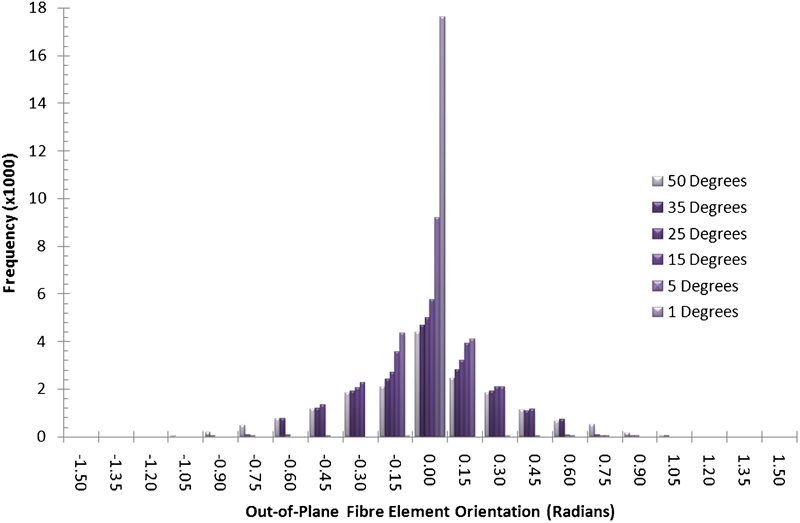
Histogram of out-of-plane orientations for fibre elements for different user specified maximum permissible angles

Figure 9 shows examples of the maximum principal stress (MPS) field and the corresponding damage field for one of the simulated coupons. Areas shaded blue on the damage plot signify elements with an MPS value under the yield strength of the resin (elastic region). Green areas indicate elements beyond the yield point within the plastic region of the stress–strain curve. Red indicates elements that have failed according to the MPS criteria, and the stiffness matrix has been reduced by a factor of 100 for each one affected. The inset image shows regions of high stress in the matrix material surrounding some of the fibre bundles. This indicates that stress transfer is occurring between the fibre bundles and the matrix according to the embedded element technique.

Figure 9

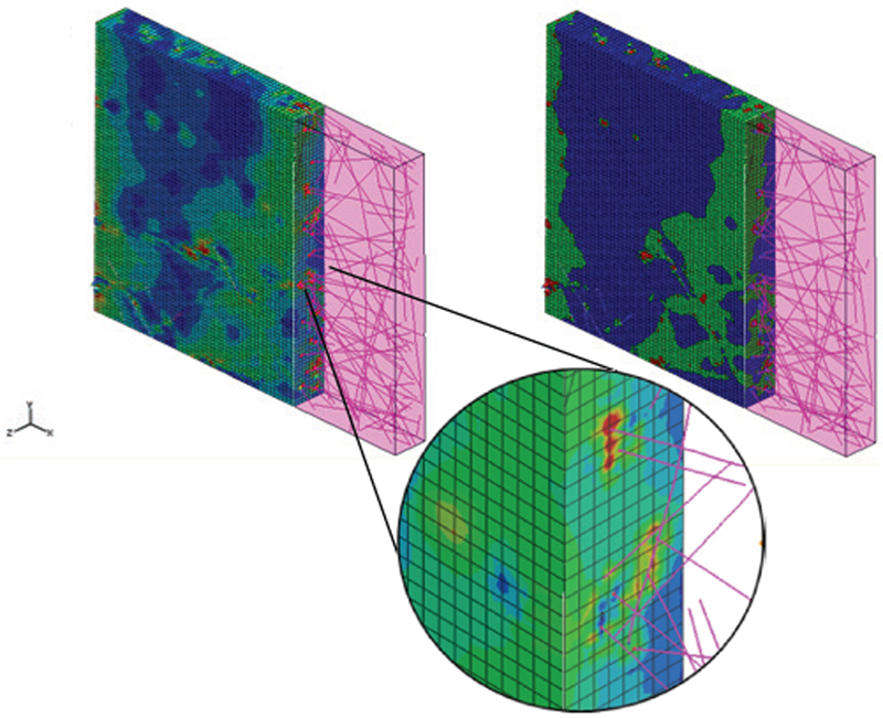
Maximum principal stress plot (left) and damage parameter plot (right) for random fibre FEA coupon (30×30×3 mm) at global applied strain of 0·75%: both images are sectioned to show internal fibre architecture

There is a small reduction (5%) in tensile stiffness with increasing levels of out-of-plane fibre curvature within the range studied, as shown by the stress–strain curves presented in Fig. 10. The stiffness is reduced from 19·3 to 18·3 GPa as the maximum permissible angle is increased from 1 to 15°, with no further reduction for larger angles.

Figure 10

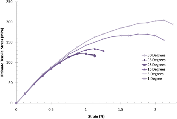
Example stress–strain curves for five coupons of same in-plane fibre distribution but increasing levels of out-of-plane curvature at fibre crossover points

Figure 11 shows a comparison of the ultimate tensile strength (UTS) predictions from the 3D FE model using the out-of-plane data from Fig. 8 and the equivalent 2D counterpart from Ref. 7. A user specified permissible angle of 0° produces a layered 2D fibre architecture, similar to that presented in Ref. 15 for direct comparison with the 2D model. There is a 14% reduction in UTS for the 3D model (assuming no out-of-plane curvature) when compared to the 2D model. Fibre to fibre intersections occur within the 2D model, providing local load sharing at fibre crossover points, reducing the local peak stress in the fibres and ultimately increasing the UTS of the 2D model. The UTS is reduced by a further 34% (Fig. 11) as the maximum out-of-plane orientation is increased from 1 to 35°. The UTS does appear to converge, however, as the threshold for the permissible out-of-plane orientation increases. This can be attributed to the shape of the orientation distribution in Fig. 8, which is approximately constant for maximum out-of-plane angles above 35°, implying that this is the practical upper limit for the out-of-plane angle in a moulded part. This study highlights the sensitivity of the UTS predictions to out-of-plane fibre orientations and the need to quantify the level of curvature witnessed in experimental test coupons. At this time, this can be confirmed by the X-ray CT scanning data from experimental coupons, but the out-of-plane distribution is expected to be a function of the number of fibre segments within the volume of material being studied (controlled by V_f, fibre length and tow size) and the degree of fibre alignment.

Figure 11

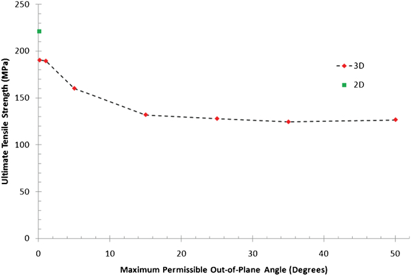
Ultimate tensile strength as function of out-of-plane orientation: first data point on left (green square) is taken from Ref. 7 using 2D embedded beam element model

Conclusions

A numerical model has been developed, offering the ability to characterise the fibre architecture of macroscale discontinuous fibre architectures in 3D and capture out-of-plane fibre bundle curvature effects. A combination of deposition algorithms has been integrated to provide a non-contacting fibre network of randomly distributed fibre bundles within a 3D space. Only the spines of the fibres have been modelled to permit high fibre volume fractions (>50%) to be modelled, with no restriction on fibre bundle AR.

RVEs generated by the model have been imported into the commercial FEA software package ABAQUS/Standard for subsequent processing. Preliminary results show that increasing the levels of permitted out-of-plane fibre curvature had little effect on in-plane tensile modulus, but the UTS decreased by up to 34% when varying the levels of curvature from 1 to 35°, with no further reduction for larger angles. The model was compared against a 2D model,7 and a technique for quantifying experimental orientation distributions has been discussed, which can be imported into the model to reconstruct physically representative fibre architectures.

Fibres have been modelled as 1D truss elements and hosted within 3D continuum resin elements using the *Embedded element technique (ABAQUS/Standard). While this methodology was chosen because of its efficiency, the processing time of the FEA has subsequently increased by two orders of magnitude compared with the 2D regime7 (using a 2·33 GHz dual core processor) because of the additional degrees of freedom. However, this approach is considered to be essential for modelling compression and flexural load cases, where fibre curvature can dominate the failure mode.

Footnotes

Acknowledgements

This research was conducted as part of the RAYCELL project and funded by Bentley Motors Ltd. The authors would like to acknowledge A. Dodworth and his team from the ‘New Technology Division’ at Bentley Motors Ltd for their continued support.

This paper is part of a special issue on Latest developments in research on composite materials

References

Turner

, Harper

, Warrior

, Rudd

: ‘Low cost carbon-fibre based automotive body panel systems – a performance and manufacturing cost comparison’, Proc. IMechE D , 2008, 222D, (1), 53–64.

Chavka

, Dahl

: ‘P4 preforming technology development utilizing e-glass and carbon fibers’, Proc. SAMPE Int. Symp., Detroit, MI, USA, May 1999, SAMPE.

Harper

, Turner

, Warrior

, Rudd

: ‘Automated preform manufacture for affordable lightweight body structures’, Proc. 26th Int. SAMPE Europe Conf., Paris, France, April 2005, SAMPE, 214–219.

‘Hexcel Product data sheet – carbon epoxy HexMC/C/2000/R1A’, Hexel Corporation, 2008, http://www.hexcel.com/NR/rdonlyres/037544D8-2EBE-40E1-B5A2-9CFD06189753/0/HEXCELHEXMCMOULDING2.pdf; accessed 10 Feb 2011.

‘Menzolit preliminary data sheet – menzolit advanced SMC 1300’, 2004, http://www.menzolit.com/templates/rhuk_solarflare_ii/pdf/list_new/AdvancedSMC_1300.pdf; accessed 10 Feb 2011.

‘YLA product bulletin – ms-4a’, TenCate Advanced Composites USA Inc., 2009, http://www.hexcel.com/Resources/DataSheets/Brochure-Data-Sheets/HexMC_User_Guide.pdf; accessed 10 Feb 2011.

Luchoo

, Harper

, Bond

, Warrior

, Dodworth

: ‘Net-shape spray deposition for compression moulding of discontinuous fibre composites for high performance applications’, Plast. Rubber Compos.: Macromol. Eng ., 2009, 39, (3–5), 216–231.

Drugan

, Willis

: ‘A micromechanics-based nonlocal constitutive equation and estimates of representative volume element size for elastic composites’, J. Mech. Phys. Solids , 1995, 44, (4), 497–524.

Evans

, Ferrar

: ‘The packing of thick fibres’, J. Phys. D: Appl. Phys ., 1989, 22D, 354–360.

10.

Kari

: ‘Micromechanical modelling and numerical homogenisation of fibre and particle reinforced composites’; 2005, Magdeburg, Otto-von-Guericke University Magdeburg.

11.

Pan

, Iorga

, Pelegri

: ‘Numerical generation of a random chopped fiber composite RVE and its elastic properties’, Compos. Sci. Technol ., 2008, 68, (13), 2792–2798.

12.

Harper

, Turner

, Martin

JRB

, Warrior

: ‘Fiber alignment in directed carbon fiber preforms – mechanical property prediction’, J. Compos. Mater ., 2010, 44, (8), 931–951.

13.

Chen

, Xi

, Masood

, Chen

: ‘Development of automated chopper gun trajectory planning for spray forming’, Ind. Rob ., 2004, 31, (3), 297–307.

14.

Catmull

, Rom

: ‘A class of local interpolating splines’, in ‘Computer aided geometric design’, (ed. , Barnhill

R E

, Riesenfeld

R F

, ed), 317–326; 1974, Salt Lake City, UT, Academic Press, Inc.

15.

Eason

, Ochoa

: ‘Modeling residual stresses and damage initiation in discontinuous random fiber SRIM composites’, Proc. 5th Int. Conf. on ‘Computer aided design in composite material technology’, Udine, Italy, July 1996, WIT Press, 123–132.