Methodology for characterisation of glass fibre composite architecture

Introduction

The fibre volume fraction (FVF) is considered as the most crucial microstructural parameter for describing fibre reinforced composites. The parameter forms the basis for the well known rule of mixtures for determining the in-plane stiffness of a composite material, see e.g. Jones.1 Commonly, the FVF is determined on the basis of the weight fractions and the densities of the individual constituents and yields an average laminate parameter for the entire composite. However, on a local scale, the FVF attains larger values, e.g. inside individual bundles where the fibre concentration is enlarged.

It is evident that there exists other microstructural parameters that characterise a fibre reinforced composite, e.g. packing pattern, neighbouring distance, clustering, etc. Information about these parameters can be extracted from measurements on cross-sections of the given composite. Digital image analysis and processing are tools to be used to identify the material microstructure. Attempts have been made in order to characterise the full three-dimensional (3D) structure of (glass) fibre composites (FVF, fibre misalignment, waviness, fibre curvature, etc.) using a sectioning approach based on microscope images. This analysis requires great accuracy in the sectioning process and in identifying the individual fibres. The method is time consuming but serves well in order to describe the local appearance of the microstructure. This 3D characterisation has been carried out by several researchers, see for instance, Paluch2 or Clarke et al. 3 These studies also include the determination of the fibre misalignment angle inspired by the ideas of Yurgartis,4 where the misalignment angle is determined by measurements of the elliptical fibre shape that appears on an inclined cross-section compared to the principal fibre direction. Using numerical routines, Creighton et al.5 and Kratmann et al.6 determined the misalignment angle for much lower resolution images and thus saving the processing time. The difference between two-dimensional (2D) and 3D characterisation is outlined in the, to some extent, personal account of Exner.7

Based on digital micrographs of a planar and polished cross-section of a unidirectional fibre composite, this study presents a methodology which detects the spatial distribution and radii of the fibres. This mapping of the fibres is used to define a number of parameters that are considered relevant for the microstructural characterisation of fibre reinforced composites. The method is capable of analysing local regions as well as entire bundles or cross-sections. For illustrating the applicability, the methodology is applied to different glass fibre reinforced composites with varying fibre contents. The ideas presented are inspired by the review work of Guild and Summerscales,8 who discuss a number of different approaches for image analysis of fibre composites, Pyrz,9who quantitatively investigated the composite microstructure by statistical tools, and Paluch,2 who made 3D characterisation based on 2D image techniques. This stereological approach for investigating the 3D microstructure based on 2D images has been used extensively, but it seems that the methods and ideas have not been brought to any practical experience. For instance, when the composite microstructure is investigated numerically using representative volume elements, general assumptions are made on the fibre distribution and packing pattern, communal fibre distance, boundary conditions, etc. Wongsto and Li10 investigated the effect of boundary condition on the representative volume element and made numerical simulation of a random distributed fibre arrangement. The fibre randomness was further investigated by Melro et al., 11 who developed a statistically characterised algorithm to generate random composite cross-sections. The predictions from the algorithm in terms of effective composite properties agreed well with the experimental data. The idea of random fibre distribution was also used by Mishnaevsky and Brøndsted,12who, in a numerical study, considered fatigue damage of unidirectional fibre reinforced composites. Ongoing work will extend the knowledge of the interplay between fatigue damage and fibre architecture since details in the fibre architecture has proven to be detrimental for fatigue performance.

Method

Shape detection algorithms are well known within the field of digital image analysis, and there exists numerous algorithms depending on the purpose. A common procedure is the Hough transformation by Hough,13 who came up with the idea of shape detection of lines based on parameter space. The work was further developed by Duda and Hart,14 where the shape detection was extended to include circular objects. This method is commonly referred to as the circular Hough transformation, and a more profound presentation can be found in the work of Shapiro and Stockman.15 The magnitude of the parameter space for shape detection depends on the shapes considered. For instance, line detection uses a two-parameter space (slope and intersection), circle detection 3 [centre (x, y) and radius] and ellipses 5 [minor/major axis, centre (x, y) and orientation]. Increasing the parameter space heavily increases the computational requirements. The current method is based on the circular Hough transformation for detection of circular shapes.

The analysis is split up into three different steps: preprocessing, processing and post-processing, as presented in Fig. 1 and the following subsections.

OPEN IN VIEWER

Figure 1

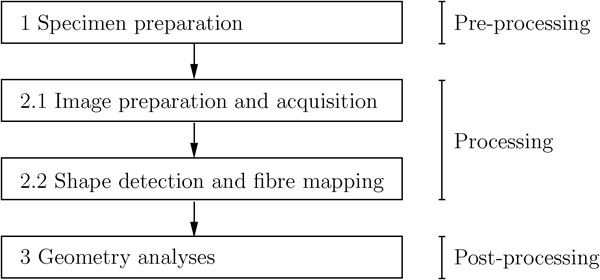
Flowchart for detection of composite microstructure

Processing

To obtain the best image quality, it is recommended to use a scanning electron microscope (SEM), an environmental SEM or a low vacuum SEM for image acquisition. If an SEM is used, the specimens need to be coated due to their non-conducting surface. It is possible to use an optical microscope, but this requires even more sensitivity in the preprocessing step due to the lower resolution, lower depth of field and poorer lighting conditions in an optical microscope compared to an electron microscope. In the present work, a low vacuum SEM is used.

The magnification of the microscope should be adjusted so the misinterpretation in the radii detection is reduced (see further discussion in the section on ‘Implementation’). To minimise computational requirements, the shape detection is based on 8 bit greyscale images. Upon acquisition of the micrographs, the shape detection is divided into two independent steps: a Canny edge detection of the image16and a circle detection based on these edges using the circular Hough transformation. The Canny edge detection locates edges by searching for a local maxima of the colour gradient within the considered image. An example is illustrated in Fig. 2, where the grey level intensity is illustrated along a given path in the image. It is evident that the edges of the fibres are detectable due to the obvious colour gradient.

OPEN IN VIEWER

Figure 2

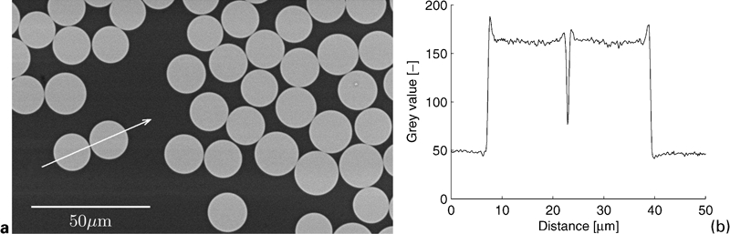
Identification of fibre edges in unidirectional (UD) fibre reinforced composite based on SEM image

Once the edges of the fibres are detected, the circular Hough transformation is applied by a voting procedure to identify the best matching circles. The input parameters for the transformation can be adjusted depending on the image quality (threshold level, search range and magnitude of search filter). The results of the detection are the in-plane fibre location (x, y coordinates) and the fibre radius r.

Owing to the numerical processing power, there is a limit for the image size that can be analysed by the circular Hough transformation. Therefore, for larger image sizes (approximately larger than 1000×1000 pixels), the entire image is split up into a number of user defined segments that are analysed separately, and the results are stored for each segment. An average value for the entire image is evaluated once all the segments have been analysed. The segmentation procedure can also be used to characterise the microstructure across a fibre bundle, the effects of clustering due to stitching tension, etc.

Post-processing

Circle sets on a plane are defined if the positions and radii of the circles are known. Characterising these circle sets requires knowledge about the number of circles, circle diameter distribution, communal distance between the circles, clustering, packing pattern and circles in contact. When these parameters are known, it is possible to make a full characterisation of the circle set. The following analyses are considered based on the fibre centre and radii obtained from the circular Hough transformation:

i.

global FVF

ii.

void content

iii.

fibre diameter distribution

iv.

number of contact points per fibre

v.

nearest neighbour distance

vi.

fibre clustering parameter

vii.

number of neighbours and local FVF.

Each of the above analyses is outlined in the following.

(i) The FVF is considered a fundamental parameter, which is used in characterising and calculating the mechanical properties of fibre reinforced composites. In the present work, the FVF is determined using three distinct procedures:

1.

knowing the individual fibre radii and the total image size, it is possible to determine the FVF of the detected fibres. It is assumed that the position and diameter of the fibres do not vary in the normal direction of the fibres. Hence, the FVF is determined as (1) where V is the volume, A is the area, N is the number of fibres and r_i is the individual fibre radius. This procedure for determining the FVF is referred to as FVF1

2.

a simple procedure to evaluate the FVF is by threshold analysis. The image is transformed into a black/white image, whereas the resin appears as black pixels and the fibres as white pixels. The FVF is found as the ratio between the white pixels and the total number of pixels. This procedure is referred to as FVF2

3.

it is likely that the circular Hough transformation does not detect every fibre in the cross-section, especially near the image boundary where the fibres are cut off. This procedure simply removes the detected fibres (used in procedure 1) and performs a threshold analysis (as in procedure 2) on the remaining undetected fibres. This procedure is referred to as FVF3.

It is given that the sum of the FVFs from procedures 1 and 3 should match procedure 2.

(ii) Voids may be present in the materials, and these voids are known to influence the mechanical properties. Since voids appear as black regions in the micrographs, these are identified if a pixel value is lower than a user defined threshold. The total void content is found as the sum of these pixels in relation to the total number of pixels.

(iii) It is often assumed in numerical analyses of fibre reinforced composites that the fibre diameter distribution is uniform, which is often not the case in practice. The fibre diameter is measured by the circular Hough transformation and assumed normal distributed, meaning that it is characterised by the mean value and the standard deviation.

(iv) Contact between surfaces leads to stress concentrations; therefore, contact between fibres is considered as a potential zone for crack initiation, see e.g. Wongsto and Li.10 A contact condition between two circles (fibres) is defined if the centre to centre distance between two adjacent circles i and j d_ij is less than the sum of their individual radii r_i+r_j. However, due to fibre surface roughness, interface and inaccuracy in the circle detection, the contact condition is given as d_ij⩽(r_i+r_j)α, where the factor α = 1·01 follows from the work of Mishnaevsky and Brøndsted.12 Denoting the total number of circle contact conditions as c, the total number of contact points CP_total is determined as (2) where the factor of 2 is included to avoid repeated contact points.

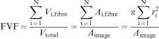
Since the total number of contact points in equation (2) is dependent on the number of inclusions, the total number of contact points is normalised with the number of detected fibres N in order to get the number of contact points per fibre CP. For two common fibre packing patterns, the number of contact points per fibre and FVF is illustrated in Fig. 3 for an infinite fibre array.

OPEN IN VIEWER

Figure 3

Typical fibre packing patterns in unidirectional composite along with FVF and number of contact points per fibre (CP)

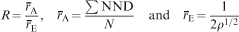
(v) Separation distance between the fibres may minimise the stress concentration, and this analysis determines the distance to the nearest neighbour. The neighbouring distance between fibres i and j is defined as ND_ij = d_ij−r_i−r_j, and the shortest distance is found by the solution to the classical travelling salesman problem (TSP) using a TSP algorithm. Further information on the TSP can be found from Lawler et al.17 The result of the analysis is the ‘shortest route’ through all fibres and thereby the nearest neighbouring distances (NNDs). For quantification, the NND is assumed to follow a log normal behaviour with mean μ and standard deviation σ, meaning that the limits are expressed as exp[log (μ)±log (σ)].

(vi) Clustering of fibres leads to regions that influence the mechanical behaviour. In order to estimate the fibre clustering, the simple relation from Clark and Evans18 is used as a measure for fibre clustering. Originally, the theory was used in terms of spatial relations in populations, but it is directly applied in the current study even though there are some limitations. The clustering parameter R is expressed as (3) with being the mean of the series of distances to the nearest neighbour, and is the mean distance to the nearest neighbour expected in an infinitely large random distribution with density ρ. In the current case, the sum of the NNDs ΣNND is found as the ‘'shortest route'’ between fibre centre mentioned above. The fibre density is found as ρ = N/A_image.

The convenient thing about the clustering parameter is its easily accessible interpretation since it is bound by the limits 0⩽R⩽2·15, where the lower limit follows from an intermediate neighbouring distance equal to 0 (fully clustered), and the upper limit is for a hexagonal array with equidistant distance to other neighbours. For R = 1, the packing pattern is random.

(vii) Often, when modelling the composite microstructure, an idealised fibre packing pattern is assumed to be in the arrays shown in Fig. 3. These packing patterns are seldomly found in practice, and the following analysis estimates the packing pattern in terms of the number of neighbours and a local FVF. More sophisticated methods may be used to characterise the packing pattern, e.g. the second order intensity function as proposed by Pyrz9 and Ghosh et al.19

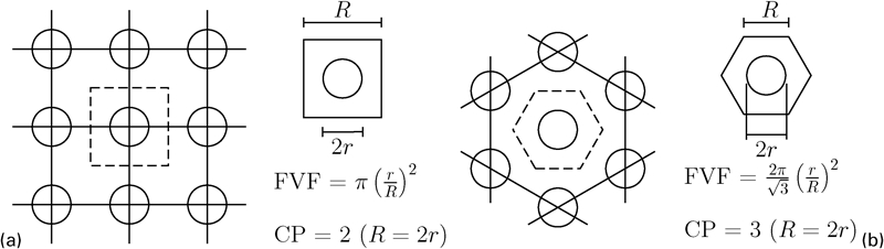
The number of neighbours is found from a Delaunay triangulation of the fibre centre points, and the local FVF is determined as the fibre area in relation to the area of Voronoi cell associated to each fibre. In brief, a Voronoi tessellation is a decomposition of a scatter (in this case points on the plane) into a cell structure each containing exactly 1 point. The property of the cell is that any point inside the cell is closer to that point than to any other site. A Delaunay triangulation, on the other hand, is sort of the dual problem to the Voronoi tessellation such that no point sets are inside the circumcircle of any triangle. The two principles are illustrated for a generated fibre arrangement in Fig. 4. For a more profound presentation, see Okabe.20

OPEN IN VIEWER

Figure 4

Sketch of Voronoi tessellation and Delaunay triangulation for random point set in plane

In the present analysis, the Voronoi cells are used to determine a local FVF (referred to FVF4) for each fibre since the area of the cell A_Voronoi can be considered as an ‘area parameter’ associated to each fibre with area A_fibre. Thereby, the local FVF is determined as A_fibre/A_voronoi. The area of the Voronoi cells along the image boundary cannot be evaluated explicitly, which is why the boundary fibres are disregarded. The local FVF is assumed to follow a normal distribution described by the mean value and the standard deviation. The centre points of the detected fibres are used as input for the triangulation in order to find the number of neighbours, here presented as the mean value and standard deviation respectively. Similar analyses have been used previously, e.g. in the work of Paluch.2

Implementation

The programming language MATLAB is used for the implementation of the methodology. The circular Hough transformation and the TSP algorithm can be found at the MathWorks File Exchange.21

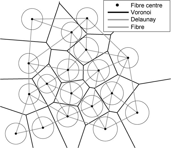
The algorithm and implementation have been tested on two selected fibres on several images with different microscope magnifications in order to estimate the accuracy of circle detection. The fibres are shown in Fig. 5a, where fibre A is completely isolated, and fibre B is surrounded by several others. The result from the analysis is shown in Fig. 5b, where the detected fibre diameter is plotted as a function of microscope magnification.

For low magnification images below 5 pixels/μm, there is a scatter in the measured fibre diameters. However, in order to get sufficient accuracy and amount of fibres per image, a value of 1·64 pixels/μm is used in the following well aware that this gives rise to a non-negligible deviation in the determination of the FVF in procedure FVF1 mentioned above.

Depending on the image shape, image size and number of fibres, the number of contact points is affected. Therefore, a test is carried out to investigate the image shape/size sensitivity. The test is carried out for a square fibre packing arrangement with no intermediate distance between the fibres. For a varying image shape/size, it turns out that for a ‘low’ number of fibres (say, <50 fibres in a narrow shaped image), the number of contact points is affected.

OPEN IN VIEWER

Figure 5

Accuracy analysis for detection of fibre radius

Application

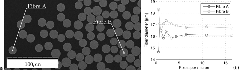
Two-layered glass/polyester composites with varying fibre contents were manufactured using the vacuum assisted resin transfer moulding process, and the specimens are analysed by the methodology outlined in the section on ‘Method’. All the images are acquired within a bundle without any resin rich zones near the edges. A typical result of the circle detection is presented in Fig. 6.

OPEN IN VIEWER

Figure 6

Typical images for analysing microstructure of unidirectional glass fibre reinforced composite: presented images are segments of analysed images

A close examination of the detected circles shown in Fig. 6 reveals that the algorithm detects a number of non-existing fibres; nonetheless, these fibres are removed in the post-processing step by evaluation of the grey level intensity at the centre of the (mis)detected fibre. The post-processing analyses are carried out as mentioned in the previous section, and the results are presented in Table 1 and Figs. 7 and 8. μ and σ denote the mean value and standard deviation respectively, and all data are assumed to be normal/log normal distributed and independent. Table 1 presents the number of detected fibres and the fibre diameter distribution.

OPEN IN VIEWER

Figure 7

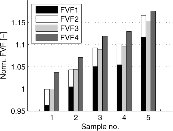
Results of image analyses: FVF based on different procedures: FVF1, radii of fibres; FVF2, boundary analysis; FVF3, threshold analysis; FVF4, local (Voronoi)

OPEN IN VIEWER

Figure 8

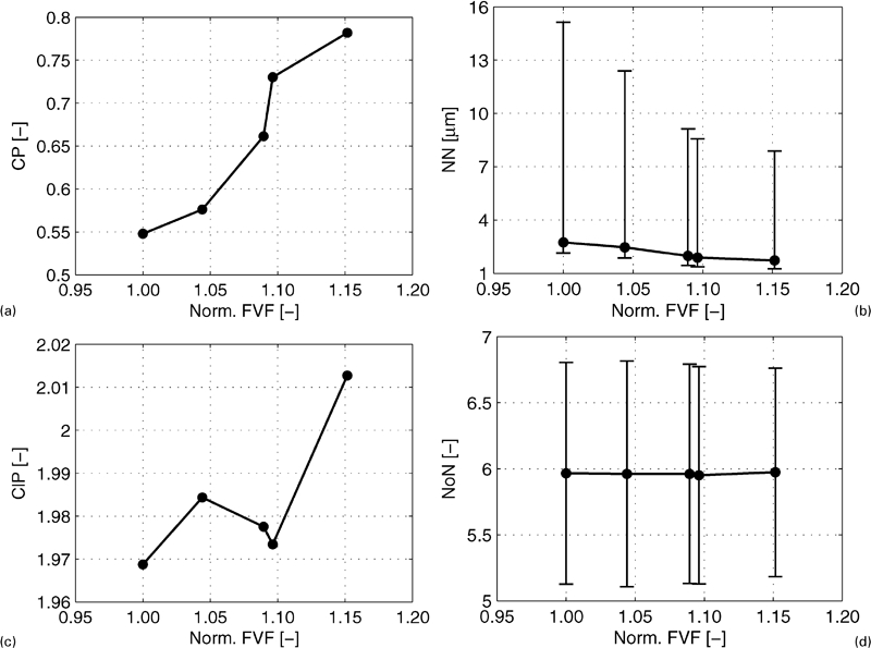
Results of image analyses for different FVFs

OPEN IN VIEWER

Table 1

Result of image analysis: number of detected fibres and fibre diameter distribution (mean μ and standard deviation σ)*

No.	NoF	FD [μ/σ] / [μm/μm]
1	4745	17·19/1·46
2	4605	17·17/1·45
3	4797	17·21/1·57
4	3335	16·96/1·44
5	7679	17·32/1·50

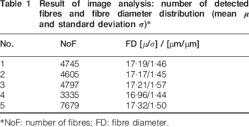
*NoF: number of fibres; FD: fibre diameter.

Figure 7 presents the obtained FVFs for the different analyses, and the results are normalised with the value from FVF3 (threshold analysis) in sample 1.

Figure 8 shows the number of contact points per fibre CP, the nearest neighbour distance NN, the clustering parameter ClP and the number of neighbours NoN as a function of the obtained FVF. Again, the FVF is normalised with the value from FVF3 (threshold analysis) in sample 1.

The variation in fibre diameters is small, and the measurements are almost constant in the range around , which is also the prescribed diameter by the manufacturer.

As mentioned in the previous section, the sum of the FVFs determined from procedures FVF1 and FVF2 should be equal to the FVF determined by procedure FVF3. This is illustrated in Fig. 7, where the deviation between the methods is within ±1·2%, which is regarded as a sufficient accuracy in the shape detection. It is worth noticing that the local FVF, i.e. FVF4, is consistently larger than the FVFs determined from the other analyses. No voids are found in the samples investigated.

For a heavier fibre compaction, it is found that the number of contact points per fibre CP increases and the nearest neighbour distance NN decreases (see Fig. 8). The packing pattern remains the same independent of the FVF, which is reflected in the number of neighbours NoN and the clustering parameter ClP approaching the upper limit of 2·15. This means that the packing pattern converges against a pseudohexagonal array.

Discussion

From the number of fibres detected (see e.g. Table 1) and the image sizes used, the image size sensitivity in relation to the number of contact points per fibre is limited for the samples considered. The number of contact points per fibre increases for increasing FVF, which is in accordance to what is reported by Mishnaevsky and Brøndsted12in a numerical study.

Even though the actual fibre packing in Fig. 6 does not appear to be systematic, the fibres tend to arrange in what is referred to as a pseudohexagonal packing pattern. Using the Delaunay triangulation, Paluch2 made a similar conclusion in relation to the packing pattern.

Pyrz9 carried out a quantitative study on the microstructure of composites based on statistical analyses. In specific, a probability investigation was made between the NND for different FVFs. The trend is obviously that the larger FVF is, the smaller the mean NND and standard deviation is observed. The same findings are concluded in the present study.

The clustering parameter described in the work of Clark and Evans18 is determined based on the fibre centre without information regarding the fibre radius. Therefore, the basis of using this analysis is misleading since the underlying statistical theory is based on point sets rather than circles. It has not been possible at this stage of the study to find a suitable description for clustering of circles where the individual radii are included.

It is apparent that it would be more accurate to determine the Voronoi diagrams in terms of circle sets on a plane rather than points due to the circular cross-section of the fibres, see e.g. presentation by Kim et al.22 However, based on the work of Paluch2 and to ease the implementation, the presented method is considered to be sufficient.

The local FVF (FVF4) predicts a larger value compared to the global FVF, which is in contradiction to what could be expected from the idealised fibre arrangements in Fig. 3that produce similar results for local and global FVFs. Still, the magnitudes of the deviation are in similar range to what is found from Ghosh et al.19 based on simulations of uniform fibre distributions with FVF in the range up to 32·4%.

The optimum solution to the TSP has been investigated by several researchers, and there exist numerous different solution techniques for the problem. However, the problem of finding the optimum solution is far from trivial. In the case of N fibres, the number of different routes is given as (N−1)!/2, which indicates the increasing problem complexity for large N. Therefore, approximated methods are often used where the route might not be the optimum one but somewhat close to. Such an algorithm is used in the present, and as a result, the shortest route might not be the optimum.

Conclusions

A new methodology is presented dealing with shape detection and microstructural analysis of composite materials containing circular fibres. Based on digital micrographs and numerical image processing, the fibre architecture/microstructure is evaluated for a number of different parameters. For demonstration, the methodology is shown useful to identify and compare microstructural parameters for different glass fibre reinforced composites with varying fibre contents. The following microstructural parameters are affected by changes in the FVF: the number of contact points per fibre, nearest neighbour distance and the local FVF (the fibre area in relation to the area of the associated Voronoi cell). For increasing FVF, the number of contact point per fibre increases, whereas the nearest neighbour distance decreases. The local FVF is somewhat larger than the global FVF. Voids are not found in the samples. Independent of the FVF, the fibres are arranged in a pseudohexagonal array with approximately six neighbours per fibre.