Strain measurement of softened Eucalyptus regnans wood during bending operation using a low-cost single camera optical method

Background

Investigations of wood stresses and strains generated during a bending operation (i.e. wood bending mechanics) are limited in number. Kollmann and Cote (1968) provide a summary of the most prominent investigations by Prodehl (1921), Stevens and Turner (1970), Fessel (1951) and Teichgräber (1953). Other notable experimental work was carried out by Peck (1957) and Makinaga et al. (1997).

Prodehl (1921) investigated stress versus strain for unsteamed and steamed beech in tension and compression parallel-to-grain. The work showed a substantial change in compression parallel-to-grain behaviour between unsteamed and steamed beech, where the steamed beech samples reached an ultimate compressive strain over 35%, whereas the unsteamed samples indicated failure below 5% compressive strain. Conversely, the increase in ultimate tensile strain between the unsteamed and steamed beech sample was only 1%. Further experimental evidence of this difference between the tensile and compressive parallel-to-grain behaviour of steam-softened wood is shown in Stevens and Turner (1970). Compression experiments showed an increase in compressive strain of steamed beech relative to unsteamed beech of nearly 30%. However, tensile performance was only slightly improved through steaming with an increase of approximately 0·3%. Teichgräber (1953) investigated the effect of steaming time and moisture content on compressive properties of beech. Teichgräber showed that a moisture content of 22% produces an increase of ∼1% in compressive strain when compared to a moisture content of 12%. Far more significant is the outcome from Teichgräber's steaming time experiments, with a substantial improvement in compressibility using a steaming time of 30 min as compared to steaming times of 5 and 10 min. Fessel (1951) conducted an experimental stress and strain analysis on oak specimens under various bending conditions. Fessel's results demonstrate that when compared to an unsteamed specimen, the effect of steaming alters the wood stress distribution by increasing the amount of compressive shortening and reducing the level of tensile stretching.

The use of a wood support rig shows that the amount of compressive shortening is further increased and tensile stretching further reduced. Peck (1957) completed an experimental strain analysis, measuring wood strains on the surface of a 25-mm thick wood specimen bent about a form with constant radius of 66·7 mm (2⅝ inches). This was carried out by marking parallel lines 25 mm apart on the tangential surface of the specimen before bending. After performing the bend, the distance between the lines at two distinct points, the convex edge and the concave edge, was remeasured. The transverse distance across the wood thickness was also measured. Wood surface strains in both longitudinal and transverse directions were then calculated.

In a manner similar to Peck (1957), Makinaga et al. (1997) performed an experimental strain analysis on Celtis occidentalis specimens, each having thickness of 10 mm and bent about a form with radius 50 mm. ‘Lines were drawn across the grain at 100 mm intervals from their central position to measure the strains along the grain on the convex and concave surfaces as well as the radius of curvature after bending.’ Following bending, the specimen was held in place and dried for 24 h at 105°C. Distances between the drawn lines were remeasured and strains calculated. Makinaga states that the longitudinal strains on the convex and concave surfaces were about 2% and −11% respectively, which shows that the steel strap of the wood support rig changed the distribution of stress in the resulting system, resulting in the wood specimen being mostly stressed in longitudinal compression.

Available strain measuring methods

Strain measuring techniques that could potentially be adapted for a wood bending process, identified in various references (e.g. Dally and Riley 1991; Williams and Ryall 1993), include strain gauges, microgridding, thermography and optical strain measurement.

Applicability of strain measuring techniques to wood bending

Contact-based techniques, such as resistance strain gauges, are not ideally applicable for a wood bending application, due to difficulties associated with wood specimens being heated, having high moisture contents and undergoing high magnitudes of strain (Sliker 1971; Dally and Riley 1991). Additionally, contact-based techniques can typically be used only once and require considerable effort to install. Fibre-optic and Rubbery Ruler strain measuring techniques, while unaffected by electrical and electromagnetic interference, can be employed to measure only longitudinal compression and tension strains and not shear strain (Li and Ansari 2001).

A non-contact strain measuring approach is therefore considered the most suitable for a wood bending operation. As well as offering a non-contacting application, thermography approaches offer benefits such as full-field measurement and high-resolution strain measurement performance. However, they are relatively expensive (Smith 1996) and calibration is likely to be difficult due to material dependency, wood variability and wood temperature variation during softening.

The optical approach to strain measurement was found to be the most appropriate; however, existing commercial systems can be prohibitively expensive for research purposes, hence the need for a low-cost alternative.

Low-cost optical strain measurement method

The proposed method to measure strain distributions induced during a bending operation is distinct from any existing methods reported in the published literature.

The method is based on the strain measurement approach used by Peck (1957) and Makinaga et al. (1997), involving ruled lines to form a grid and a manual process (ruler) to measure grid distances before and after a bending experiment.

The proposed method applies the general principals reported by Austrell et al. (1995) to wood bending operations and has the following features:

The strain measurement technique of measuring dot displacements used in Austrell et al. (1995) is a piece-wise approximation of strain on a surface. This approximation is analogous to a finite element strain calculation, where each dot represents a vertex of a finite element (Kythe and Wei 2003; Krishnaswamy 2005). During a finite element strain analysis of an object, by discretising the object's surface with a series of finite elements, strains can be estimated over the complete surface area of the object. During object deformation, vertex displacements are used to calculate associated strains within each finite element area. Finite element shapes (i.e. the configuration of the vertices or dots) can take a number of forms, including: triangular and quadrilateral. Austrell et al. (1995) applied triangular-shaped finite elements, which when compared to quadrilateral-shaped elements offer a simpler but less accurate solution under certain analysis applications including bending deformation (Krishnaswamy 2005).

In this study, custom code was developed from scratch as Austrell et al. provided only a basic structure and some key algorithms for the dot's ‘image intensity’ but no details of coding in their paper. The code was also adapted where appropriate to accommodate the different equipment and user processes required for bending strain analysis.

Optical strain measurement function

The customised optical strain measuring system (OSMS) consists of a digital camera mounted to record digital images of a wood specimen during bending (Fig. 1a). The specimen has a strain grid introduced to its surface, consisting of painted white dots forming a grid over a painted black background on the appropriate surface and location of a wood specimen. During bending, wood deformation causes the white dots to move and the digital camera records these dot displacements through a series of images of the strain grid as the associated load is increased. The recording process includes an initial, undeformed image before deformation of the specimen. A light source is directed onto the strain grid to enhance measurement accuracy. An infrared remote control is used to activate the recording operation for each digital image to prevent camera vibration through user contact. Custom-designed computer software uploads the digital images, determines relative dot displacement, and calculates induced strain. [Details of the strain measuring system methodology and associated customised computer code are provided as Supplementary Material 1 (Supplementary Material 1 http://dx.doi.org/10.1179/2042645312Y.0000000017.s1).]

OPEN IN VIEWER

Figure 1

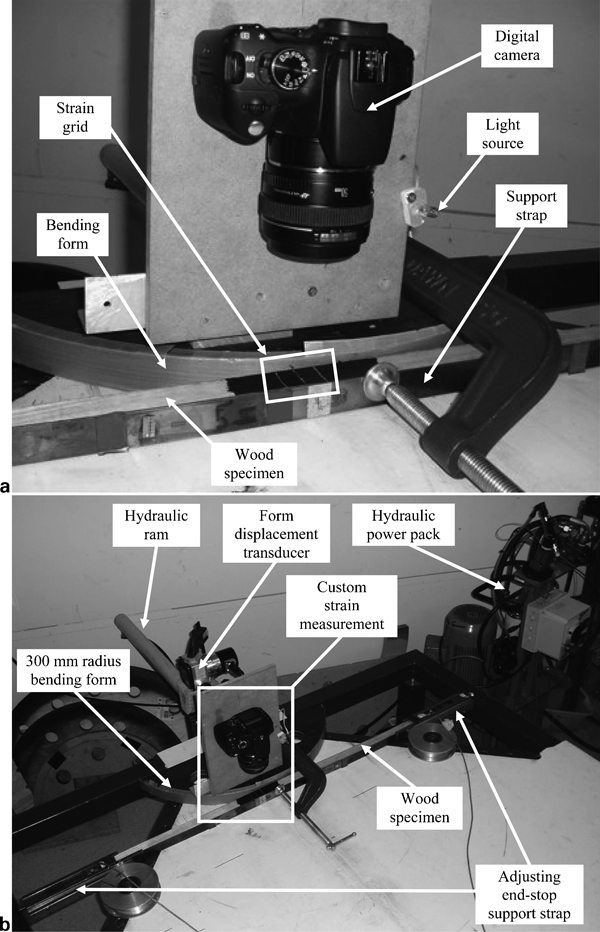
a components of the custom-designed strain measuring system and b laboratory equipment used to complete inexpensive strain analysis experiments. Distance between strain grid on wood surface and end of camera lens (closest point of the lens to strain grid) was ∼85 mm. This distance, combined with the range of vision of the camera system, determined the conversion factor between wood distance and image pixels. During strain analyses, the conversion factor was ∼75 mm/pixel. Camera specification: Canon EOS 350D digital camera with a Canon 50 mm EF lens. Image size: 3456×2304 pixels. The light source (12 V LED), combined with the ambient fluorescent laboratory lighting, was acceptable to ensure constant and uniform light conditions

Strain grid installation

The technique for applying the black background to the surface of wood specimens is important due to difficulties associated with the softening and relatively high moisture contents of the wood specimens as wood moisture can permeate the wood surface during softening and impair the applied strain grid. A matt-finish (as opposed to a gloss-finish) is required to ensure that the black background is ignored by the computer vision software when completing ‘centre of area’ calculations.

A process for applying a black background was successfully developed, involving the application of a base of carbon black stain followed by a light coat of a matt-finish, black-coloured spray paint. After the black background paint has dried, the grid of white dots is applied using a single hair from a fine-haired brush to apply a white-coloured, oil-based paint. This grid system facilitates strain measurement in the longitudinal, transverse and shear directions on the surface of a wood bending specimen (Fig. 2).

OPEN IN VIEWER

Figure 2

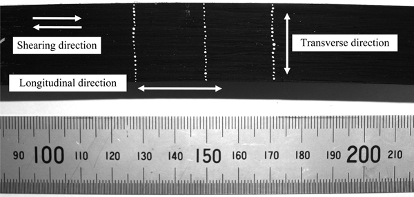
Strain grid applied to wood specimen (zoomed view of grid shown in Fig. 1a. Strain measurement directions are indicated. Metric rule indicates grid scale

Computer software code

After bending, the recorded digital images of the strain grids are uploaded from the camera into a computer, where the custom-designed strain measuring software code is used to process the strain grid images and calculate wood surface strains.

The computer software reads in two images at a time and calculates the wood strains generated between these two images (i.e. strain generated between the two associated form displacements). Only successive images are processed by the software (i.e. image nos. 1 and 2 are processed, then image nos. 2 and 3 are processed, and so on until the last two successive images). This process provides a change in strain value for each pair of strain grid images (i.e. at each successive form displacement), and in so doing, demonstrates strain development throughout the bending operation, and offers a stepwise approach that reduces possible error associated with divergent non-linear strain development when compared to processing images with the undeformed strain grid always first (i.e. image nos. 1 and 2 are processed, then image nos. 1 and 3 are processed, and so on until the end of the bending operation).

The semi-automated strain measuring software prompts the user to select a set of four dots within the strain grid of the first of two uploaded images that require the calculation of mean strain values at a specific wood thickness in the longitudinal, transverse and shear measurement directions (Fig. 2) over the area enclosed by the four dots. After dot selection is complete, the software calculates the relative position of each of the dots using a centre of area (COA) calculation (Fig. 3). The COA calculation for each dot is based on a function involving a first-order area moment and the light intensity of the associated strain grid image (Austrell et al. 1995).

OPEN IN VIEWER

Figure 3

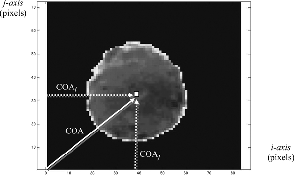
Example of a photographed dot (Fig. 2) after the COA calculation process is applied by the strain measuring computer software. The various shades of colour (image shown in greyscale) correspond to the different light intensities of the white dot that are captured during the digital image recording process. The (reasonably central) white square (enlarged for illustrative purposes) represents the pixel that corresponds to the COA position of the dot. The solid white arrow (COA) represents the COA position vector that is calculated for each dot selection during the four-dot selection process. The dashed white arrows represent the components of the COA positional vectors in the i-axis and j-axis directions

The software then prompts the user to select the same four dots in the second image that were selected in the first image, and a second set of four COA values are calculated using the COA calculation. The software then subtracts the two sets of COA vectors from each other to determine relative dot displacements. The relative dot displacements, together with absolute position vectors of each dot from the first image, are used in a finite element calculation to determine the mean surface strain values associated with the selected four dots in the longitudinal, transverse and shear directions (Fig. 2). Finite element calculations are based on Krishnaswamy (2005).

Strain as a function of wood thickness can be developed by repeating the above four-dot selection process for a series of locations across wood thickness.

Light conditions on strain grid

Light conditions imposed on the strain grid throughout a strain analysis need to have a constant and reasonably uniform intensity, as the certainty of dot location by the image capture and dot location algorithm (i.e. COA calculation) depends, in large part, on the performance of the camera vision system, of which the lighting is a critical factor. A change in the light intensity during a bending operation can alter the camera's view of the digital image, and therefore, adversely affect the relative position of the associated dots and their strain calculation. To ensure appropriate light conditions are applied during an experimental strain analysis, two processes are implemented.

First, a constant direct current light source is directed at the strain grid. Despite this, light conditions can still vary, for example, due to specimen deflection out of the major deflection plane during bending.

Second, application of an additional customised algorithm to detect and accommodate changes in light conditions. This algorithm is based on an assumption that a dot's shape and associated density of light should not change significantly from image to image during a bending operation if light conditions are constant. Any relatively large change in the dot's shape or density of light detected by the algorithm is then attributed to altered light conditions (Fig. 4).

OPEN IN VIEWER

Figure 4

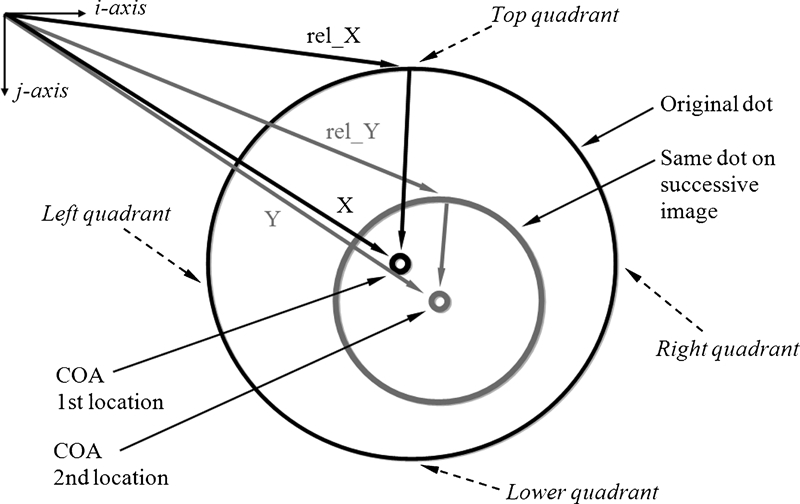
Schematic showing dot vectors used in light condition computer algorithm test code. Position vectors measured from local origin. If light conditions are acceptable, rel_COA_X and rel_COA_Y are approximately equal (within a tolerable error margin)

Light conditions potentially have an excessive affect when:

•

the ‘estimated light strains’ are significantly greater than 0·1%. (this percentage represents the minimum strain resolution that is considered acceptable for the OSMS during strain analyses)

•

the ‘shape change factors’ are significantly greater than 1·13 pixels (this value represents the minimum allowable displacement of a dot during strain analyses – introduced in the section on ‘Performance trial no. 1’ to follow)

•

the estimated light strains and shape change factors are within similar magnitude to the actual calculated strains and dot displacements.

Under these conditions, the associated strain analysis is considered for rejection. Successful calibration trials were completed to ensure this light condition algorithm functioned correctly (Juniper 2007). The light condition algorithm provides an enhanced confidence in the accuracy of the strain measurements reported.

Optical strain measurement performance trials

Two sets of experiments were completed to assess the performance of the OSMS:

Trial no. 1: comparing the accuracy of reported displacements against those measured by a commercial material testing machine to identify intrinsic system errors

Trial no. 2: assessing the effect of vibration due to external excitation of the experimental strain analysis rig and internal camera shutter on the measurement performance.

Performance trial no. 1

The OSMS is configured to record digital images and calculate displacements of a single dot located at the moving crosshead of the material testing machine. The performance of the OSMS is assessed by comparing the dot displacements to the corresponding material testing machine crossheads displacement.

After an initial digital image of the dot at the crosshead's starting position was recorded (i.e. when the displacement of the moving crosshead is zero), the crosshead was moved a short distance, and a second image was recorded. This second image was compared to the initial digital image, and the associated displacement of the dot was calculated between the two using a customised computer algorithm. The actual crosshead position relative to its original position was also recorded using the internal instrumentation of the material testing machine. The position error, relative to actual displacement, of the strain measuring system (SMS) for a specific crosshead movement, or dot displacement, was calculated using (1) The process of moving the crosshead a short distance, recording an image, and calculating position error, was repeated until the decreasing position error value was satisfactory. The results from this trial (Fig. 5) showed that at material testing machine crosshead displacements greater than 0·015 mm the position error associated with the OSMS remains practically constant. Hence, to ensure strain measurements have an associated low intrinsic error, the minimum acceptable displacement recorded by the OSMS is 0·015 mm (or 1·13 pixels) [conversion between millimetres and pixels based on a factor of 75 mm/pixel which is the approximate wood distance per number of camera pixels for the camera arrangement (i.e. distance between lens focal point and wood surface) used in the strain analyses (Fig. 1)].

OPEN IN VIEWER

Figure 5

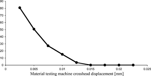
Dot displacement position errors associated with the SMS compared against a commercial testing machine (Instron Universal Testing Machine). The minimum acceptable displacement recorded by the SMS is 0·015 mm

Performance trial no. 2

To complete an assessment of the effect of vibration on OSMS performance, a mock experimental strain analysis was configured, but not performed. The digital camera was rigidly installed on the bending form and a wood specimen in an unsoftened condition was located in its wood support rig and assembled into the bending machine. A single dot was positioned on the specimen and two consecutive digital images of the dot were recorded.

A customised vibration assessment computer algorithm was used to find the COA positional vectors of the two dots. A non-zero difference between the COA vectors is attributed to vibration effects because there are no other options for COA variation (i.e. room temperature is maintained at a constant level and no load is applied to the specimen) (Fig. 6).

OPEN IN VIEWER

Figure 6

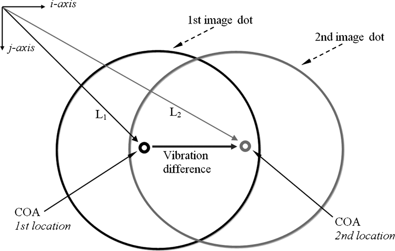
Schematic image of vibration assessment trial. If a non-zero difference exists between L₁ and L₂, it is attributed to vibration effects

Output from the vibration assessment computer algorithm provided the COA positional vectorial equations of each dot.

The vibration difference associated with COA images was calculated using (2) where Δx_pos is difference in the i-direction between the two position vectors and Δy_pos is difference in the j-direction between the two position vectors.

The vibration difference (Δ_{COA pos}) represents the magnitude of the vibration effect, and if small enough relative to the displacement being measured, has an insignificant adverse effect on the performance capacity of the OSMS.

Based on a series of trials, the average vibration difference was found to be 0·0043 mm (0·341 pixels). This is less than the minimum acceptable displacement of the OSMS (i.e. 0·015 mm, performance trial no. 1), and as such, vibration effects have no significant impact on experimental outcomes when the OSMS is used during experimental strain analyses.

Optical strain measuring system: Gauge lengths for strain grid

A suitable gauge length for the OSMS strain grid is best determined by:

A minimum gauge length for each strain measuring direction is calculated using (3) Longitudinal strain magnitudes were previously measured in the order of 2% at the convex edge and −11% at the concave edge (Peck 1957; Makinaga et al. 1997). Assuming similar outcomes using the OSMS, detection of maximum longitudinal strains would require a gauge length of 0·75 mm for the convex edge (i.e. using equation (3), gauge length ⩾0·015/0·02). However, to detect incremental changes in longitudinal strain during a bending operation and not just the overall strain of a completed bending operation, a larger gauge length is required to maintain acceptable strain measuring accuracy. Preliminary strain analysis trials showed that strain incremental changes in the order of 0·1% should be measured during a bending operation as this provided enough accuracy to effectively establish a relationship between strain development and bending form displacement. Hence, a minimum gauge length of 15 mm (i.e. 0·015/0·001) in the longitudinal direction was found to be required to maintain the minimum acceptable displacement.

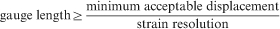
The expected magnitude of transverse strain is less well known. Peck (1957) claims to have measured compressive transverse strains of up to 4%. However, preliminary strain analysis trials conducted measured changes in transverse compressive strains during a bending operation as low as 0·1%. Consequently, the detection of strains to within 0·1% requires a minimum gauge length in the transverse direction of 15 mm (i.e. using equation (3), gauge length ⩾0·015/0·001). This minimum gauge length restricts potential investigations into the variation of transverse strain across the thickness of wood specimens with a (nominal) 25 mm thickness, hence a mean transverse strain across the majority of the specimen could be calculated instead.

As shear strain is a function of both longitudinal and transverse strain (Krishnaswamy 2005), the shear strain minimum gauge length is determined by the minimum gauge lengths for the longitudinal and transverse strain directions. The 15 mm minimum gauge length for the transverse direction dictates that shear strain will also be measured over the majority of the (nominal) 25 mm thick wood specimen. This gauge length, and associated strain resolution for the shear direction, is inadequate as shear strain is known to vary with a component's thickness when under flexure loads (e.g. Avallone and Baumeister 1997), and similar observations with wood specimens are expected during a bending operation.

Experimental wood strain analyses using OSMS

For best performance, it was found that the digital camera of the OSMS should be installed on the bending form of a bending machine in a position directly above the strain grid location (Fig. 1b), with the appropriate zoom and aperture settings established. A single manual lens adjustment focuses the image of the specimen's strain grid (the same focus needs to be maintained throughout the bending operation). Then, an initial digital image of the undeformed strain grid is recorded. The bending form is then displaced incrementally and a second digital image is recorded. The displacement of the form can be recorded by a commercially available data acquisition system and displayed in real-time on a computer screen to assist positioning. The process of displacing the form and recording a digital image is completed for a series of form displacements as required. Displacement increments should be selected with reference to the following issues:

During the bending operation, the form should be displaced at a constant speed to ensure that the specimen has enough time to respond to the bending deformation that is being imposed on it, due to the visco-elastic properties of the softened wood. End-stop adjustments using the wood support rig can be made if required (this depends on the underlying objective of the experiment). If maximum wood strain magnitudes are sought, end-stop adjustment should not take place. A moisture content sample can be obtained near the vicinity of the strain grid from the bent component using the moisture content determination method described in AS/NZS 1080·1:1997 or equivalent international standard.

The process required to obtain and subsequently analyse the measured strains (Fig. 7) begins with uploading the undeformed and initial form displacement strain grid images into a computer. The custom-designed strain measuring computer software can then be used to calculate the strains depending on strain direction:

OPEN IN VIEWER

Figure 7

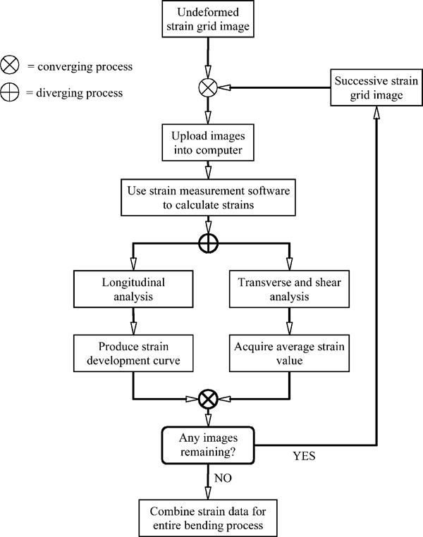
Flowchart illustrating the tasks required to find wood specimen surface strains during experimental strain analyses

Longitudinal: The four-dot selection process is repeated across the thickness of the wood specimen associated with the strain grid (transverse-direction in Fig. 8) to provide a piecewise longitudinal strain development curve relative to wood thickness.

OPEN IN VIEWER

Figure 8

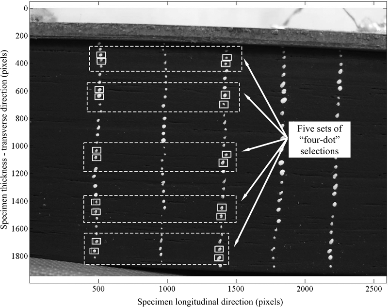
Example of the four-dot selection process enabling longitudinal strain calculation at five different locations across the wood thickness. This four-dot process is conducted at different locations across the wood specimen's thickness to determine a piecewise strain development curve. The resulting strain data is used to construct a strain development graph (e.g. Fig. 11)

Transverse, shear: A single, four-dot selection process is made using a set of dots where the upper and lower two dots are within the vicinities of the concave and convex edges of the specimen (Fig. 9) to determine mean transverse and shear strain values across the majority of the wood specimen.

OPEN IN VIEWER

Figure 9

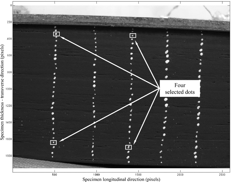
Example of the four-dot selection process for transverse and shear strain. The distance between the dots in the wood specimen's transverse direction extends across the majority of the wood specimen to assist obtaining the required mean transverse and shear strain magnitudes. The resulting strain data enables the construction of a strain development graph (e.g. Fig. 11)

These strain calculations can be repeated for each successive form displacement until the end of the bending operation.

The same set of dots is selected for each successive strain grid digital image throughout a strain measurement for each bending operation.

The practical application of OSMS

If the experimental conditions are such that the end-force is adjusted to maintain the development of strain at a level just below the wood's ultimate strength, and optimum bending conditions are maintained, the results from an OSMS can provide a set of engineering properties that specify the ultimate strain magnitudes that can be imposed on a wood specimen during bending for a given specimen cross-section and bending method.

Knowing the engineering properties that govern the behaviour of a material is crucial for proper and efficient use of the material. A general definition of an engineering property is an intrinsic or attributive property of a material that characterises the material's associated engineering performance and function, appearance, cost and workability (Ashby and Jones 1996). Engineering properties are only obtained through experimentation (Timoshenko 1955). They are commonly used to define an aspect or characteristic of a material for use during some specific application of the material (Shackelford 2005).

Hence, the ultimate strain magnitudes from the OSMS would allow production of bent-wood components with the smallest possible bending radius without incurring any wood failure. This can assist the future design of:

Before determining ultimate strain magnitudes, the combination of salient wood bending variables and end-force conditions imposed on a wood specimen to produce optimum bending performance must be found.

Four engineering properties can be determined using the OSMS technique:

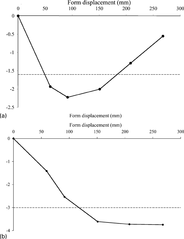
For each engineering property, a graph of strain versus form displacement can be constructed to show how the engineering strain property varies through the duration of a bending operation (for example, Figs. 10 and 11).

OPEN IN VIEWER

Figure 10

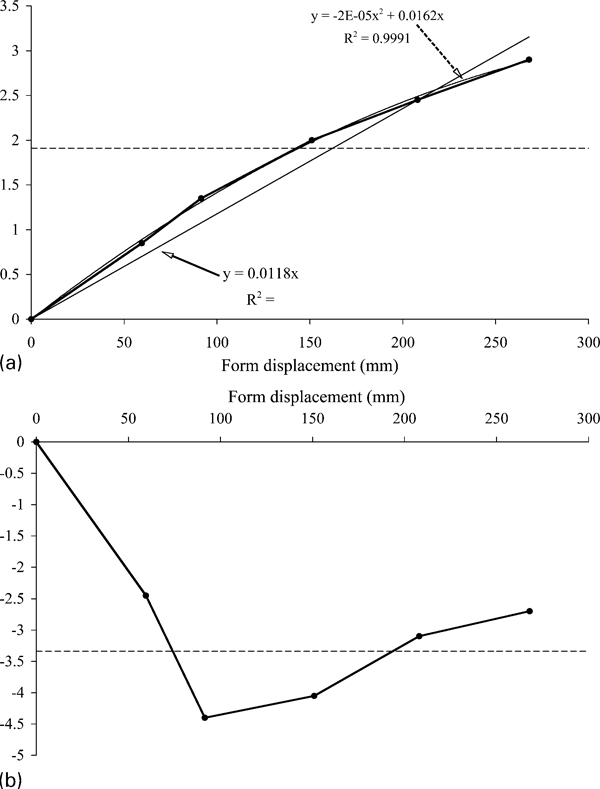
Typical strain development graphs (across the sample) for a sample of 25 mm² specimens of Eucalyptus regnans during bending. a mean longitudinal strain at convex edge during bending progression and b mean longitudinal strain at concave edge during bending progression. Horizontal lines in both graphs represent the sample longitudinal strain means: convex edge = 1·91%, concave edge = −3·34%

OPEN IN VIEWER

Figure 11

Typical strain development graphs for a sample of 25 mm² specimens of Eucalyptus regnans during bending. Mean strains, averaged across the specimen transverse thickness during bending. a transverse strain and b shear strain. Horizontal lines in both graphs represent the sample strain means: transverse = −1·60%, shear = −3·01%

It has been found that wood strain can remain constant once the post-bend-phase (associated with the location of the strain grid) has been reached (Juniper 2007), because:

After the section of wood containing the strain grid has been bent to the form, the applied end-force is constant and, as such, no further increase in wood strain should occur.

When considering data distributions, highly dispersed data associated with the ultimate strain engineering properties can be attributed to one or more of the following inherent variational factors:

Concluding remarks and recommended future enhancements to OSMS

A low-cost single-camera optical based method for measuring engineering strain has been introduced. The method requires minimal specialised equipment and has been successfully trailed in the determination of engineering properties of Eucalyptus regnans (Juniper 2007).

Currently, the OSMS is a semi-automated system, but it is envisaged that future development could facilitate a fully automated system by enhancing the strain measuring computer software and incorporating appropriate equipment to:

Also, as the strain resolution of digital cameras improves, incremental (i.e. at a series of form locations during a bending operation) variation in strain across wood specimen's thickness during bending could be introduced.