Liquefaction-Induced Lateral Spread in Lo Rojas,Coronel,Chile: Field Study and Numerical Modeling

Abstract

This paper describes a detailed field survey conducted at Lo Rojas fishermen port in Coronel, where extensive liquefaction-induced lateral spread was reported for the 2010, M_w 8.8 Maule earthquake. The survey includes SPT and SCPT soundings, as well as the use of surface-based geophysical techniques. The data was used to evaluate a multilinear regression (MLR) lateral-spread expression and to develop a detailed hydro-mechanical finite element model. Results of the MLR equation were over-conservative and proved to be very sensitive to the distance from the site to the energy source. On the other hand, the results from the numerical model agreed reasonably well with the post-event field observations.

INTRODUCTION

The 27 February 2010 M_w 8.8 Maule earthquake caused important damage to ports and bridges, considerably affecting the economic activities of the country. In many cases, this damage was associated with liquefaction-induced lateral spread phenomena, in which large masses of soil slide over a liquefied layer, imposing large displacement demands on existing structures.

Caleta Lo Rojas, located 25 km south of Concepción, is a fishermen's wharf that showed clear evidence of liquefaction-induced lateral spread. The most damaged structure was a pier, which had to be replaced after the earthquake (Figure 1). The large horizontal displacements that affected the area produced the complete failure of the old pier (Figure 1b). During a post-earthquake reconnaissance (Bray et al. 2012), estimates of cumulative horizontal displacements were measured by summing the crack widths along the line indicated in Figure 1a. A lateral movement of at least 2.85 m was estimated across a distance of about 85 m (Figure 1c).

Figure 1.

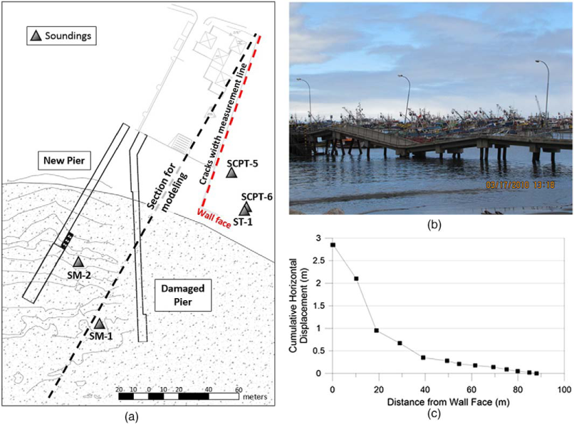
(a) Lateral spread measurement line and location of geotechnical soundings; (b) damaged pier; (c) cumulative horizontal ground displacements.

In the present study, an extensive survey was performed to characterize the site and then simplified, and advanced modeling methods were applied to verify if they were able to reproduce the observed post-seismic displacements. The survey included seismic geophysical methods, SPT and SCPT soundings.

The information collected during the field reconaissance and explorations is used to make a detailed soil characterization, and to develop a geotechnical two-dimensional (2-D) soil profile of Lo Rojas area. A multilinear regression empirical equation (Youd et al. 2002) and a fully coupled nonlinear numerical model are used to estimate residual lateral spread displacements. The results using both methods are then compared against post-seismic observations, and a discussion on their relative weaknesesses and strenghs is presented.

EXPLORATION BOREHOLES

Boreholes SM-1 and SM-2 were drilled for the construction project of the new wharf in 2010, next to the old pier that was severely damaged during the earthquake (Figure 1b). Each borehole had a depth of about 25 m from the mean sea level. An additional borehole, ST-1, was drilled in 2014 to a depth of 20 m from a relative elevation of 2.87 m above sea level. Additionally, two seismic cone penetration tests (SCPT-5 and SCPT-6) were performed. Boreholes and SCPT locations are shown in Figure 1a.

Figure 2a displays the normalized blow count (N ₁)₆₀ values. Results from SM-1 and SM-2 were corrected assuming an energy efficiency of 60%, while for ST-1 the energy was recorded during the SPT tests with an average energy ratio of 68.9% and a standard deviation of 4%. Using the available bathymetry, absolute vertical elevations to mean sea level were computed for each borehole. The results show a sharp contrast between the upper and deeper soils. ST-1 shows that the transition from soft to denser material occurs at about 14 m below sea level, while the marine soundings indicate that this transition takes place at about 20 m below sea level.

Figure 2.

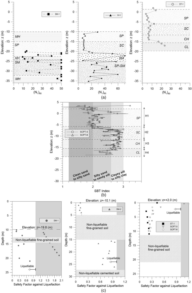
(a) Stratigraphy and comparison from three boreholes (ST-1, SM-2, and SM-1); (b) SBT Index from SCPT soundings; (c) safety factor against liquefaction with fines correction (Youd et al. 2001) from available soundings.

Figure 2b displays soil behavior type (SBT) from SCPT borings according to Robertson (2010). The data indicates two dominant materials in the first 20 m: sand and clay. There is a transition between these two soils as the SBT values show. The upper 8 m are mainly clean sands that progressively change to silty sand for the following 4 m, and then turn into clayey silt to silty clay at about 10.5 m below the surface. The (N ₁)₆₀ values for the first 20 m are fairly uniform with blow counts of less than 10 blows/ft. Also, the USCS classification from ST-1 samples (Figure 2a) agrees with the SBT index, showing very similar transitions and designations. With such low values of (N ₁)₆₀, conventional liquefaction assessment methods predict liquefaction down to the interface with the clay or clay-like layers. The Factor of Safety against liquefaction (FSL) was calculated from the SPT and SCPT measurements (Figure 2c), considering fines content corrections (Youd et al. 2001) with a peak ground acceleration of 0.4 g, based on the ground motion recorded in the downtown Concepcion station (PGA = 0.402 g, http://terremotos.ing.uchile.cl/). Calculations using approaches proposed by Idriss and Boulanger (2006), Cetin et al. (2004), and Robertson and Wride (1988) yield the same zone of liquefaction in the vicinity of ST-1/SCPT5 and SCPT6.

Bray and Sancio (2006) proposed limits to define if fine-grained soils are likely to liquefy or not, based on the results of cyclic testing. According to these authors, if the plasticity index (PI) is larger than 20 or the moisture content (w _c) is lower than 0.8 times the liquid limit (LL) value, the material is not susceptible to liquefaction. Clay layers CH and CL meet at least one of these conditions: the CH layer has a PI of 28.3, and the CL layer has a maximum w _c/LL ratio of 0.75, likely defining the depth limit for the liquefiable behavior. This is also supported by the Idriss and Boulanger (2006) criteria, which indicates that fine-grained soils will exhibit clay-like behavior if they have a PI ≥ 7. Since the SC layer had an SBT index of I _c > 2.6, and its fines fraction had a plasticity index PI > 11, layers between an elevation of −6.5 m to −19 m (referenced from mean sea level) were considered non-liquefiable in this study.

Granulometric curves from the ST-1 boring shown in Figure 3 exhibit a clear progression from coarse to fine soils. The fines content varies progressively from 1% in the first 6 m, to 70% at 15 m below sea level.

Figure 3.

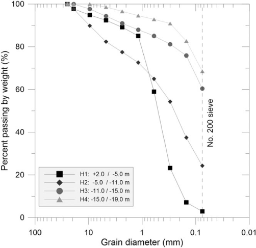
Average granulometric curves for each stratum.

GEOPHYSICAL SURVEY

The geophysical survey in Caleta Lo Rojas included two areas, labeled SW-1 and SW-2 (Figure 4). Two different geophone arrays were used on each area. Additionally, the Horizontal to Vertical Spectral Ratio (Nakamura 1989), or HVSR, was calculated at six points. From the HVSR plots predominant frequencies, f ₀, and amplitudes, A ₀, can be obtained (see Figure 5b). The predominant frequency, f ₀, is an estimator of the fundamental vibration frequency of the site, while the amplitude of the HVSR, A ₀, directly correlates with the impedance contrast between upper soft layers and deeper stiff layers. Figure 4 shows the f ₀ values that were obtained. The values for A ₀ where rather homogeneous, ranging from 4.9 to 6.7, which show a distinct contrast between soft and stiff deposits.

Figure 4.

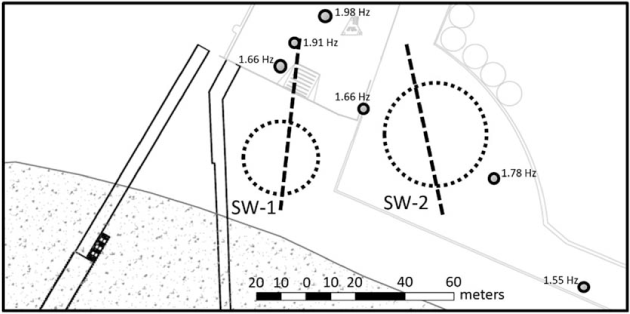
Geophysical survey: Nakamura results and explored area.

Figure 5.

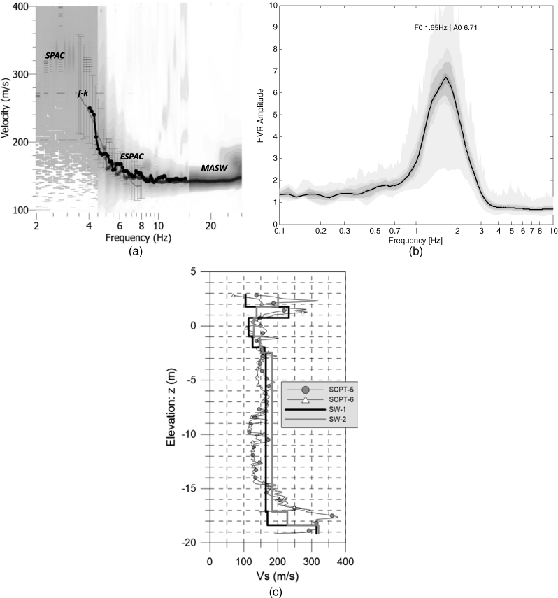
(a) Dispersion curves from SW-2 area; (b) example of HVSR ratio; (c) shear wave profiles (two sites and comparison with SCPT).

Seismic surface wave–based geophysics methods characterize dispersive properties of a site using both, passive sources (ambient vibrations) and active sources (sledgehammer). For this investigation, we used a seismograph of 24 channels with two kinds of geophones (natural frequencies of 4.5 Hz and 1 Hz). Lower frequencies imply longer wavelengths which allows deeper exploration. In this case, due to the very low shear wave velocities of the soil, the use of 1 Hz geophones was essential to reach at least 30 m of depth. The performed analyses assumed only Rayleigh waves. For source-controlled experiments (active tests), we used the multichannel analysis of surface waves (MASW) method (Park et al. 1999). For ambient noise measurements (passive sources), we used SPAC (Aki 1957) and f-k methods (Lacoss et al. 1969) in the case of bi-dimensional arrays. Additionally, for the analysis of passive linear measurements, we used the extended SPAC (ESPAC) under the assumption of isotropic incident fields (Hayashi 2008).

Figure 5a shows the dispersive properties of the SW-2 area, combining the results of SPAC, f-k, ESPAC, and MASW methods along a linear and a circular array. Agreement between the different techniques is very satisfactory and allows characterization of the dispersion curve between 2.5 Hz and 30 Hz, approximately. It is important to note that geophysical surveys do not characterize a specific point, but they represent an average across the area covered by the arrays. Once a dispersion curve is obtained, the inversion must generate a model of horizontal soil layers with elastic properties compatible with the field observations in terms of the dispersive characteristics (dispersion or autocorrelation curves). In this work, we used the extension of the Neighborhood Algorithm (NA; Sambridge 2001) proposed by Wathelet (2008) to solve the inverse problem. The results of the application of this method to areas SW-1 and SW-2 are shown in Figure 5c. The results are compared against “direct” measurements subsequently performed with the seismic cones SCPT-5 and SCPT-6 (see Figure 1a). The shear wave velocity profiles obtained from the geophysical survey have a very good agreement with the profiles obtained from the SCPT measurements.

Figure 5b shows a typical result of HVSR. The large amplitude peak implies the existence of a clear stiffness contrast at a given depth. The mean fundamental frequency for this site is f ₀ = 1.66 Hz, with an average shear-wave velocity down to 20 m of V _S = 160 m/s (see Figure 5c). If the well-known formula V _S = 4 Hf ₀ is used, these measurements show that the impedance contrast should be located at a depth of 24 m from the soil surface, which is in good agreement with the depth reported in Figure 5c. Even if this stiffer material detected by Nakamura's method is not the bedrock, this stiffness contrast defines the predominant vibration period for this site.

GEOTECHNICAL MODEL

To estimate lateral spread using both empirical and detailed numerical methods, a geo-technical model of the area was developed. The adopted geotechnical model (Figure 6) was based on all the available information with respect to soil profiles, results from the geophysical investigation, and the bathymetry that was provided by the Ports Department of the Ministry of Public Works.

Figure 6.

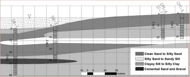
Geotechnical model of the cross section through the slope.

The bathymetry shows a pronounced slope of about 11% close to the coast, a necessary condition to develop liquefaction-induced permanent ground displacement.

The profile is characterized mainly by three materials: H1 (clean sand to silty sand), H2 (silty sand to sandy silt), and H3 (clayey silt to silty clay). Additionally, a lens of cemented sand and gravel was assumed based on the SM-1 borehole information. Material H1 is liquefiable, while the material H2 was assumed as non-liquefiable due to the increase of fines content and plasticity index with depth. H3 is considered to be non-liquefiable. For the sand and silty sand layer (H1), marine borings SM-1 and SM-2 show erratic values of factors of safety against liquefaction below z = −20 m (Figure 2b). The material at this depth is probably too dense to liquefy, therefore, for the lateral spread assessment presented in the next two sections, it was assumed that H1 material located below z = −20 m could not liquefy.

EMPIRICAL PREDICTION OF LIQUEFACTON-INDUCED LATERAL SPREAD DISPLACEMENTS

Based on the information presented in the previous sections, multilinear regression (MLR) equations for predicting lateral spread displacement are evaluated. Although the primary focus is on revised equations published by Youd et al. (2002) which have been widely used, results from other equations are also addressed. Youd et al. (2002) suggested improvements to the Bartlett and Youd (1992b, 1995) MLR equations, such as an added constant to the distance term to prevent unrealistically large displacements, and additions to the case history database. Because the S-shaped slope at the Lo Rojas site does not clearly meet definitions of a gentle slope nor a free face scenario, both equations are evaluated and compared.

The general form of the revised MLR equation for free-face conditions is:

where R ^* = R ₀ + R, and R ₀ = 10^{(0.89M – 5.64)}. The variable, D _H, is the estimated lateral ground displacement, in meters; M is the moment magnitude of the earthquake; R is the nearest horizontal or map distance from the site to the seismic energy source (in kilometers); R ₀ is a distance constant that is a function of M; R ^* is the modified source distance; T ₁₅ is the cumulative thickness, in meters, of saturated layers with corrected blow counts, (N ₁)₆₀, less than 15 blows/ft; F ₁₅ is the average fines content (fraction of sediment sample passing a No. 200 sieve) for materials included within T ₁₅, in percent; D50₁₅ is the average mean grain size for materials within T ₁₅, in millimeters; W is the free-face ratio defined as the height (H) of the free face divided by the distance (L) from the base of the free-face to the site, in percent.

As discussed in previous sections, the liquefiable layer was determined to extend from the surface to an elevation of −6.5 m according to the SCPTs and ST-1, the closest soundings to the wall where displacement was measured. The soil from −6.5 m to −11 m below sea level is clayey sand with a PI of 11.4 and over 30% fines, indicating it is unlikely to liquefy. Subtracting the depth to groundwater, this leaves a continuous 8.7 m of saturated sand with (N ₁)₆₀ less than 15 blows/30 cm defining T ₁₅, which is consistent with the SCPT data showing a high SBT below an elevation of −6.5 m as shown in Figure 2b. Due to the scarcity of sample data from SM-1 and SM-2, fines content and grain size data were computed from averages of eight samples obtained from ST-1. Using the same layers considered for T ₁₅, F ₁₅ = 4.2% and D50₁₅ = 0.46 mm. The location of the free-face was estimated at about the location of SM-2, as the ground appears to level off at this location according to Figure 6, such that W = 10.7% for the maximum measured displacement. Because R must represent the distance to the seismic energy release, we choose, as a first approximation, the distance to the maximum uplift, although a value of 0.5 km would be selected according to the procedure specified by Youd et al. (2002) because the fault plane lies under the site. According to Vargas et al. (2011), the zone of maximum coastal uplifts was located at Piures, about 47 km from the Lo Rojas pier.

Entering these values into Equation 1, the computed horizontal displacement, D _H, is 12.4 m which is beyond the limits of the methodology. Varying the F ₁₅ and D50₁₅ values within one standard deviation ranges only changes the computed displacement by about ±15%, so these factors are unlikely to account for the discrepancy. The error is likely associated with the difficulty in selecting an appropriate R for subduction zone earthquakes. Despite the addition of the constant R ₀ = 155.6 km, it appears that the equation still produces an exaggerated estimate of displacement. The poor agreement is likely explained by the fact that only 7 of the 484 data points in the Youd et al. (2002) database involve a subduction zone event (Alaska, M_w = 9.2; Bartlett and Youd 1992a) or an M_w greater than 8.5.

Regression equations proposed by Zhang et al. (2004) and Faris et al. (2006), which employ peak ground acceleration rather than R, also overestimate measured lateral spread displacements by more than a factor of two. The best agreement is obtained with a method proposed by Zhang et al. (2012) which uses the same soil and geometric parameters as Youd et al. (2002) but correlates with spectral acceleration at 0.5 s rather than R. This required the use of a Chilean strong motion attenuation relation developed by Contreras and Boroschek (2012). Nevertheless, the measured displacement was still 1.5 times higher than the computed value. Additional details regarding these analyses are provided by Williams (2015).

Clearly, additional calibration of MLR prediction equations for subduction zone earthquakes is necessary. Because the zone of maximum uplift would be difficult to estimate, an alternate method to estimate distance to the maximum energy release zone is required. For this study, it is proposed to use the smaller distance R to a zone where slip (co-seismic displacements between plates) exceeds a given value (Moreno et al. 2010). A cumulative frequency graph was made to define possible threshold values of slip (Figure 8). Hence, for any slip threshold, an area that bounds slip larger than this value could be defined. For instance, if we are interested in the area bounding 50% of the largest slips (Zone A on Figure 7a), an equivalent threshold of about 5 m is found. Under the assumption that the amount of energy released is proportional to the slip magnitude, this area bounds the source of 50% of the released energy during the event. Once an amount of released energy is selected, the three-dimensional (3-D) distance to any location could be computed based on an interplate fault model. For this study, we selected the Slab 1.0 model of Hayes et al. (2012) displayed in Figure 7b. Based on this idea, different amounts of energy release have been evaluated to obtain a set of equivalent distances to be used in combination with Equation 1. Among these choices, best results were obtained when 10% of the largest slips are considered (zone B in Figure 7a and R _B = 89 km) with a lateral spread prediction of D _HB = 3.1 m. If 50% of the larger slips are considered, R _A = 54 km, and the prediction increases to D _HB = 7.6 m. Please note that R _A and R _B are 3-D distances.

Figure 7.

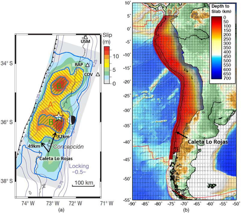
Estimation of maximum energy releasing zone: (a) USGS coseismic slip teleseismic model (Moreno et al. 2010); (b) interplate zone model Slab 1.0 (Hayes et al. 2012).

Figure 8.

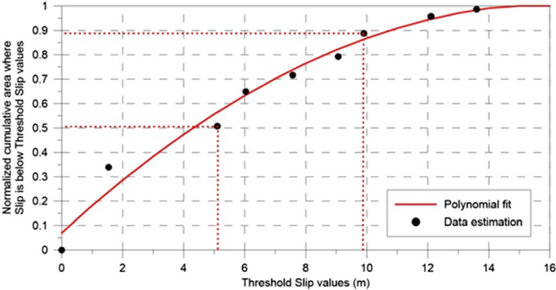
Normalized cumulative frequency of co-seismic slip over Maule earthquake rupture zone.

The parameters used for the gentle slope analysis are the same as for the free-face scenario, except the free-face ratio is omitted, and a term including S = the ground slope in percent is added. Additionally, coefficients for the gentle slope scenario are different, such that:

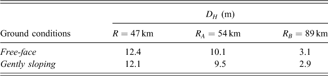
A slope S = 2.7% was estimated from Figure 6b in the vicinity of the measured displacements (approximately 40 m upslope) as suggested by Youd (personal communication). Using R = 47 km, D _H = 12.1 m which is unrealistic. Using R _A and R _B the results are D _HA = 9.5 m and D _HB = 2.9 m. The modified value R _B again provides the best estimate of the measured lateral spread. Table 1 summarizes results from both equations and all R values. Further study of the effect of the distance term or appropriate ground motion parameters for large magnitude earthquakes is suggested for future revisions of the MLR equations.

Table 1.

Horizontal displacement (m) from Youd et al. equations with original and modified values of R

NUMERICAL MODELING

Based on the geotechnical information summarized in Figure 6, we developed a fully coupled hydro-mechanic inelastic finite element model to reproduce the field observations shown in Figure 1c. In this model, the soil-fluid mixture was treated according the u-p formulation (Zienkiewicz and Shiomi 1984). This formulation neglects the fluid acceleration and its convective terms, so that the unknown variables remain the displacement of the solid, u, and the water pressure, p. Soil grain compressibility is neglected, and the behavior of the solid skeleton is derived assuming the principle of effective stress as proposed by Terzaghi. Under such assumptions, the numerical problem consists in simultaneously solving the conservation of momentum of the soil-fluid mixture, the relative flow equation, and the mass conservation equations.

The construction of a finite element mesh requires limiting the extent of the problem, both horizontally and vertically. Vertically, the model displayed in Figure 6 was extended 5 m below the bedrock, and paraxial elements were used below this level (Modaressi and Benzenati 1994). The function of these elements is twofold: On one hand, they are used to introduce the earthquake loading to the model after de-convolution from the outcropping bedrock. On the other, they absorb the waves originating inside the model due to its reflection on the surface and those at the interfaces between layers of soil. The horizontal extension of the model was limited to 260 m. This distance is large enough to capture local effects in the steepest part of the slope. Since the model is completely inelastic, traditional absorbent elements cannot be used on the vertical edges. One way to solve this problem is to use appropriate lateral boundaries to ensure “free-field” conditions far away from the slope.

As the problem is not horizontally periodic, a standard tied approach (Zienkiewicz et al. 1988) is not appropriate for this case. To impose the free-field condition at the vertical edges, three approaches were investigated: FEM-DOF, to impose displacements and pressures from a one-dimensional (1-D) propagation simulation; FEM-force, to impose equivalent lateral forces from free-field 1-D column computations (Bielak et al. 2003); and FEM-column, which adds free-field columns at the lateral edges of the full 2-D model (McGann and Arduino 2011). Approaches FEM-DOF and FEM-force require two computations: first, the free-field 1-D column must be solved and second, the equivalent displacements or forces must be imposed to the 2-D model along the vertical edges. The FEM-column approach has the advantage of requiring a single computation.

The finite element mesh used is shown in Figure 9, where each tone corresponds to a group of items, internally defined in the program, that match the different material properties that were considered. For the FEM-column approach, the mesh includes free-field columns at both vertical ends, as Figure 9 shows. In the case of the FEM-DOF/force approaches, the free-field columns are solved separately, and the 2-D model includes only the displacements or forces applied on the vertical boundaries. The mesh including the columns is composed of about 2,800 nodes and 5,300 solid triangular elements, for a total of about 8,000 degrees of freedom (mechanical and hydraulic). This finite element mesh is fine enough for the considered problem, since it satisfies the condition of having at least eight nodes per wavelength up to 10 Hz. All calculations were carried out with the program GEFDyn (Aubry and Modaressi 1996), which is capable of modeling thermo-hydro-mechanical coupled problems on static, quasi-static, as well as dynamic regimes. Once the initial stress state is computed, the seismic analysis is performed “around” the initial static situation, which corresponds to a dynamic disturbance analysis.

Figure 9.

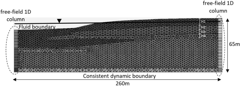
Finite element model.

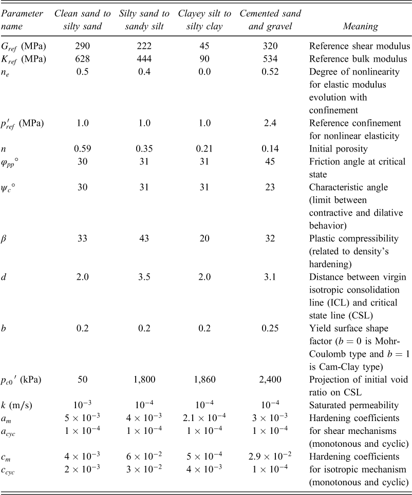
The Ecole Centrale Paris's (ECP) elasto-plastic multi-mechanism model (Hujeux 1985) was used to represent the sand behavior. This effective-stress model can take into account the soil behavior in a large range of deformations. The representation of all irreversible phenomena is made by four coupled elementary plastic mechanisms: three plane-strain deviatoric plastic deformation mechanisms in three orthogonal planes, and an isotropic one. The model uses a Coulomb-type failure criterion and the critical-state concept. The evolution of hardening is based on the plastic strain (deviatoric and volumetric strains for the deviatoric mechanisms, and volumetric strain for the isotropic one). A kinematical hardening, based on the state variables at the last load reverse, is used to take into account the cyclic behavior. The soil behavior is decomposed into pseudo-elastic, hysteretic, and mobilized domains. The ability of this model to reproduce liquefaction has been highlighted in several studies (e.g., Lopez-Caballero and Modaressi 2008, 2010; Sáez and Ledezma 2015). Nevertheless, several other constitutive model are able to model liquefaction and associated lateral spread (e.g., Prevost 1985, Yang et al. 2003, Byrne et al. 2004, Boulanger and Ziotopoulou 2012, Wang and Xie 2014). Sands and silt models, consistent with the SPT/SCPT data from the site, were selected from the authors' materials library. Material parameters for the soils used in the model are displayed in Table 2.

Table 2.

Parameters of the ECP model for the considered materials

To study the influence of the treatment of the vertical edges on the liquefaction-induced lateral spread, we selected the NS component from the Rapel station. This station is located approximately 350 km northeast of Lo Rojas, and the record has a duration of about 90 s and a PGA of 0.2 g. Figure 10a shows the accelerogram of this record, and Figure 10b shows the 5%-damping pseudo acceleration response spectrum (EW component is also included in this plot). The computed PGA at the ground surface varied between 0.3 g and 0.5 g within the laterally spreading area, with an average value of 0.38 g. Figure 11a displays the excess pore pressure ratio R _u contour plots at t = 80 s for the three explored approaches. It can be noted that complete liquefaction takes place approximately in the same zones, regardless of the adopted approach. In the case of the FEM-DOF approach, pore pressure increments seem to involve deeper materials when compared against the other two computations. Only in the case of the FEM-force approach, liquefaction shows some discontinuity close to the toe of the slope. Despite these minor differences, results are qualitatively very similar.

Figure 10.

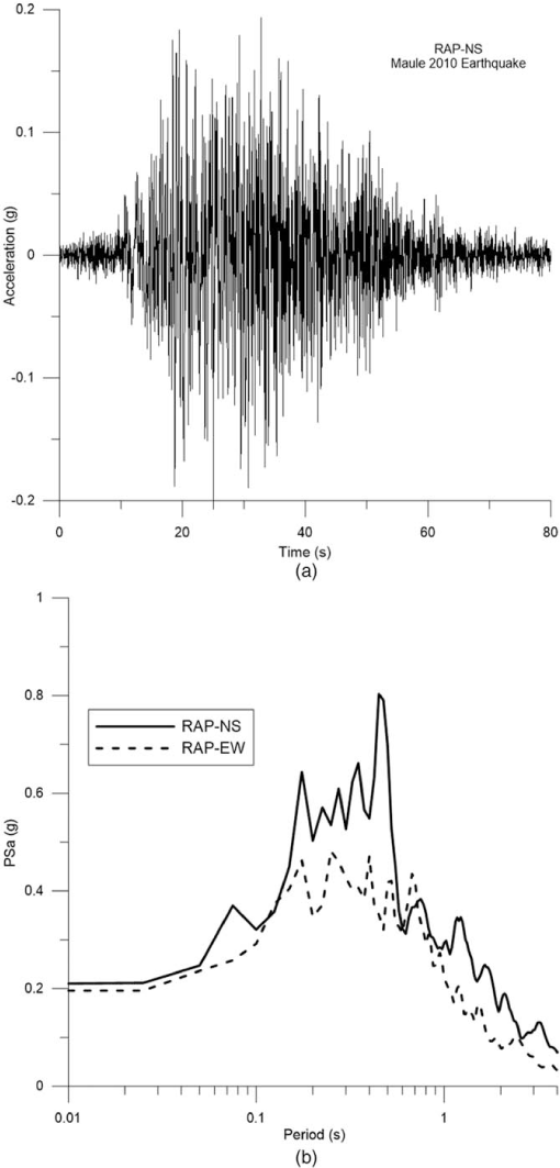
Selected ground motion: (a) accelerogram of the NS component; (b) 5%-damping pseudo acceleration response spectra.

Figure 11.

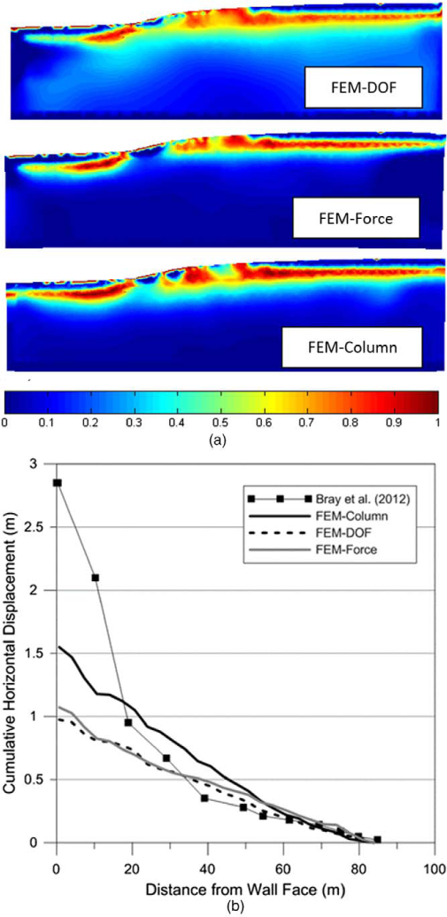
Boundary conditions benchmarking: (a) pore pressure ratio Ru contour maps; (b) cumulative horizontal displacement.

For a more quantitative comparison, Figure 11b shows the cumulative horizontal displacements measured across the projection of the line measured by Bray et al. (2012) over the section considered for modeling. In terms of maximum values, the FEM-column approach provides the closest value when compared against field measurements (about 57% less than the total cumulative horizontal displacement). Results from FEM-DOF and FEM-force models are identical for practical purposes. It is interesting to note that the measured cumulative displacements between 20 m to 80 m from the wall face are very similar to those obtained using the FEM-column model, but the large displacement increment that takes place in the first 20 m is not properly captured by the numerical model. It is likely that the wide cracks observed in the field cannot be reproduced by a continuous modeling strategy such as FEM.

SENSITIVITY OF COMPUTED DISPLACEMENTS TO INPUT MOTION

To assess the sensitivity of the results to the selection of a particular ground motion, the model was rerun using multiple input motions. To make the results as general as possible, all the available rock ground motions from the Chile 2010 event were considered even though some of them are probably affected by topographic effects. Since all the recordings had different fault-to-site 3-D distances, they were scaled, component-by-component, to the same PGA's of Rapel station (RAP). The ground motions that were used, their locations, distances to the fault plane, PGAs, and scaling factors, are provided in Table 3. The results from these analyses (range and average trend of results) are shown in Figure 12.

Figure 12.

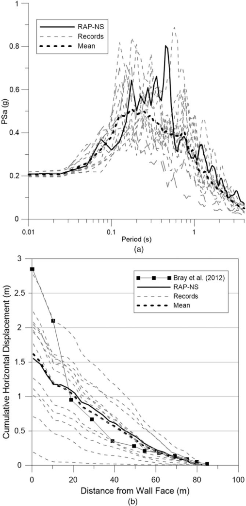
Sensitivity of the computed displacements to the selected input ground motion: (a) 5%-damping pseudo-acceleration response spectra; (b) cumulative horizontal displacements.

Table 3.

Available records for sensitivity analysis

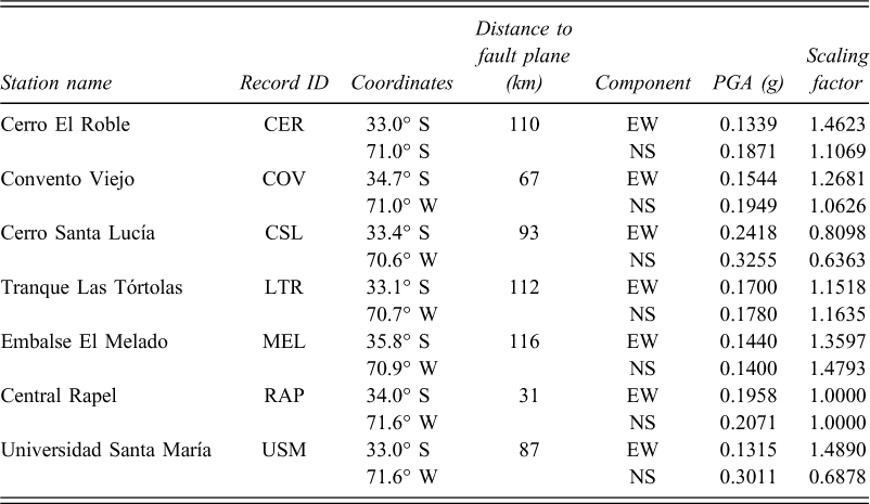
Figure 12a shows the 5%-damping pseudo acceleration response spectra of the scaled ground motions compared to the NS component of the Rapel station. Spectral ordinates are similar for periods below 0.1 s and above 2 s, but differences of up to 0.7 g can be noted in the mid-range. These differences partially explain the variability of the lateral spread predictions shown in Figure 12b. Predicted cumulative horizontal displacements were typically in the 1 m to 2 m range, however one of the records produced a very low value (0.2 m for the USM-NS record), whereas another (COV-EW) approximately replicates the maximum observed in the field, but with a different rate of displacement accumulation. The results of the unscaled record that has a similar fault-to-Lo Rojas 3-D distance (RAP-NS) approximately matches the mean values of both, the pseudo acceleration response spectra, and the cumulative horizontal displacement, probably influenced by the fact that this motion's PGA was selected as a target value for all the records. Because all the computations have almost the same PGA, variability of the results illustrate that this ground motion intensity parameter is not a good predictor of the lateral spreading phenomenon, and that a proper lateral spreading estimation procedure must consider other characteristics of the ground motion such as frequency content and duration. Also, as expected, these results highlight the importance of the proper selection of input ground motions for this type of analyses.

CONCLUSIONS

In the present study, an extensive survey including geophysical methods, SPT, and SCPT soundings was conducted to characterize the site of Caleta Lo Rojas in Coronel city, where large seismically induced lateral spread was reported for the Maule 2010 earthquake. The information indicates that the site is characterized by a steep slope of about 11% along approximately 90 m. The shallowest soil layer is characterized by 7 m of low-density silty sand to clean sand, followed by about 5 m of clayey sand. Below this level, the high fines content (larger than 50%) defines a boundary with non-liquefiable material. Based on this information, simplified and advanced modeling approaches were applied to reproduce the observed post-seismic displacements.

Empirical prediction equations prove to be extremely sensitive to the distance from the site to the energy source. In subduction zones such as Chile, the rupture area of large earthquakes could be several hundreds of kilometers. In this study, we adopted the distance to the maximum observed coastal uplift. Using this value, empirical predictions surpassed the available observations by a factor of about 4, but using the distance to the zone that bounds 10% of the largest slips, the results match satisfactorily with in-situ post-earthquake measurements.

The results using the FEM-column approach, as proposed by McGann and Arduino (2011), were similar to those obtained using the FEM-DOF or FEM-forces procedures, with the advantage of requiring a single computation. More analyses are required to extrapolate this result to other cases.

A laboratory testing program is currently being conducted using samples from ST-1. Based on these laboratory results, constitutive models will be recalibrated to improve the FEM results. Also, the simultaneous inclusion of the vertical component of the record will be considered in future stages of this investigation.

Footnotes

ACKNOWLEDGMENTS

This study is based upon work supported partially by the Chilean Comisión Nacional de Investigación Científica y Tecnológica (CONICYT) under Grant No. USA2012-0007, by the National Research Center for Integrated Natural Disaster Management CONICYT/FONDAP/15110017, by the Chilean Fondo Nacional de Desarrollo Científico y Tecnológico (FONDECYT) under Grant No. 11110125, and by the US National Science Foundation, Division of Civil, Mechanical, and Manufacturing Innovation (CMMI) under Grant No. CMMI-1235526. Any opinions, findings, conclusions, and/or recommendations expressed in this material are those of the authors and do not necessarily reflect the opinions or policies of the sponsors.

References

Aki

1957. Space and time spectra of stationary stochastic waves, with spectral reference to microtremors, Bull. Earthq. Res. Inst. 35, , 415– 456.

Aubry

, Modaressi

1996. GEFDyn: Manuel Scientifique , Ecole Centrale Paris (in French).

Bartlett

, Youd

1992a. Case Histories of Lateral Spreads Caused by the 1964 Alaska Earthquake , Technical Report No. NCEER-92-0002, National Center for Earthquake Engineering Research, Buffalo, NY.

Bartlett

, Youd

1992b. Empirical Analysis of Horizontal Ground Displacement Generated by Liquefaction-Induced Lateral Spread , Technical Report No. NCEER-92-0021, National Center for Earthquake Engineering Research, Buffalo, NY.

Bartlett

, Youd

1995. Empirical prediction of liquefaction-induced lateral spread. Journal of Geotechnical and Geoenvironmental Engineering, ASCE , 121, , 316– 329.

Bielak

, Loukakis

, Hisada

, Yoshimura

2003. Domain Reduction Method for three-dimensional earthquake modeling in localized regions; Part I, Theory, Bulletin of Seismological Society of America 93, , 817– 824.

Boulanger

R. W.

, Idriss

I. M.

2006. Liquefaction susceptibility criteria for silts and clays, Journal of Geotechnical and Geoenvironmental Engineering, ASCE , 132, , 1413– 1426.

Boulanger

R. W.

, Ziotopoulou

2012. PM4Sand (Version 2): A sand plasticity model for earthquake engineering applications. Report No. UCD/CGM-12/01, Center for Geotechnical Modeling, Department of Civil and Environmental Engineering, University of California, Davis, 100 pp.

Bray

, Rollins

, Hutchinson

, Verdugo

, Ledezma

, Mylonakis

, Assimaki

, Montalva

, Arduino

, Olson

, Kayen

, Hashash

Y. M. A.

, Candia

2012. Effects of Ground Failure on Buildings, Ports, and Industrial Facilities, Earthquake Spectra 28, , 97– 118.

10.

Bray

, Sancio

2006. Assessment of the Liquefaction Susceptibility of Fine-Grained Soils, Journal of Geotechnical and Geoenvironmental Engineering 132, , 1165– 1177.

11.

Byrne

P. M.

, Park

S. S.

, Beaty

, Sharp

, Gonzalez

, Abdoun

2004. Numerical modeling of liquefaction and comparison with centrifuge tests, Canadian Geotechnical Journal 41, , 193– 211.

12.

Cetin

K. O.

, Seed

R. B.

, Kiureghian

A. D.

, Tokimatsu

, Harder

L. F.

Jr. , Kayen

R. E.

, Moss

R. E. S.

2004. Standard Penetration Test-Based Probabilistic and Deterministic Assessment of Seismic Soil Liquefaction Potential, Journal of Geotechnical and Geoenvironmental Engineering 130, , 1314– 1340.

13.

Contreras

, Boroschek

2012. Strong Ground Motion Attenuation Relations for Chilean Subduction Zone Interface Earthquakes, in Proceedings in 15th World Conference on Earthquake Engineering , Lisbon, Portugal.

14.

Faris

A. T.

, Seed

R. B.

, Kayen

R. E.

, Wu

2006. A semi-empirical model for the estimation of maximum horizontal displacement due to liquefaction-induced lateral spreading, in Procceedings of the 8th U.S. National Conference on Earthquake Engineering, paper 1323 , San Francisco, CA.

15.

Hayashi

2008. Development of the Surface-Wave Methods and Its Application to Site Investigation, Ph.D. Dissertation, Kyoto University.

16.

Hayes

, Wald

, Johnson

2012. Slab1.0: A three-dimensional model of global sub-duction zone geometries, Journal of Geophysical Research: Solid Earth (1978–2012) 117, .

17.

Hujeux

J. C.

1985. Une loi de comportement pour le chargement cyclique des sols, Génie Parasismique, Presse ENPC , 287– 302 (in French).

18.

Idriss

I. M.

, Boulanger

R. W.

2006. Semi-empirical procedures for evaluating liquefaction potential during earthquakes, Soil Dynamics and Earthquake Engineering 26, , 115– 130.

19.

Lacoss

R. T.

, Kelly

E. J.

, Toksöz

M. N.

1969. Estimation of seismic noise structure using arrays, Geophysics . 34, , 21– 38.

20.

Lopez-Caballero

, Modaressi

2008. Numerical simulation of liquefaction effects on seismic SSI, Soil Dynamics and Earthquake Engineering 28, , 85– 98.

21.

Lopez-Caballero

, Modaressi

2010. Assessment of variability and uncertainties effects on the seismic response of a liquefiable soil profile, Soil Dynamics and Earthquake Engineering 30, , 600– 613.

22.

McGann

, Arduino

2011. Dynamic 2D Effective Stress Analysis of Slope, OpenSees Examples .

23.

Moreno

, Rosenau

, Oncken

2010. 2010 Maule earthquake slip correlates with pre-seismic locking of Andean subduction zone, Nature 467, , 198– 202.

24.

Nakamura

1989. A method for dynamic characteristics estimation of subsurface using micro-tremor on the ground surface, Railway Technical Research Institute 30, , 25– 30.

25.

Park

C. B.

, Miller

R. D.

, Xia

1999. Multichannel analysis of surface waves, Geophysics 64, , 800– 808.

26.

Prevost

J. H.

1985. A simple plasticity theory for frictional cohesionless soils, Soil Dynamics Earthquake Engineering 4, , 9– 17.

27.

Robertson

P. K.

2010. Soil behaviour type from the CPT: an update, 2nd International Symposium on Cone Penetration Testing, CPT'10 , Huntington Beach, CA, available at www.cpt10.com.

28.

Robertson

P. K.

, Wride

C. E.

1998. Evaluating cyclic liquefaction potential using the cone penetration test, Canadian Geotechnical Journal 35, , 442– 459.

29.

Sáez

, Ledezma

2015. Liquefaction mitigation using secant piles wall under a large water tank, Soil Dynamics and Earthquake Engineering , http://dx.doi.org/10.1016/j.soildyn.2015.06.012

30.

Sambridge

2001. Finding acceptable models in nonlinear inverse problems using a neighbourhood algorithm, Inverse Problems 17, , 387.

31.

Vargas

, Farías

, Carretier

, Tassara

, Baize

, Melnick

2011. Coastal uplift and tsunami effects associated to the 2010 Mw8.8 Maule earthquake in Central Chile, Andean Geology 38, , 219– 238.

32.

Wang

, Xie

2014. Modified bounding surface hypoplasticity model for sands under cyclic loading, Journal of Engineering Mechanics 140, , 91– 104.

33.

Wathelet

, Jongmans

, Ohrnberger

, Bonnefoy-Claudet

2008. Array performances for ambient vibrations on a shallow structure and consequences over Vs inversion, Journal of Seismology 12, , 1– 19.

34.

Williams

N. D.

2015, Evaluation of Empirical Prediction Methods for Liquefaction-Induced Lateral Spread from the 2010 Maule, Chile, Mw 8.8 Earthquake in Port Coronel, M.S. Thesis, Brigham Young University, 145 pp.

35.

Yang

, Elgamal

, Parra

2003. Computational model for cyclic mobility and associated shear deformation, Journal of Geotechnical Geoenvironmental Engineering, ASCE , 129, , 1119– 1127.

36.

Youd

, Hansen

C. M.

, Bartlett

2002. Revised multilinear regression equations for prediction of lateral spread displacement, Journal of Geotechnical and Geoenvironmental Engineering, ASCE , 128, , 1007– 1017.

37.

Youd

T. L.

, Idriss

I. M.

, Andrus

R. D.

, Arango

, Castro

, Christian

J. T.

, Dobry

, Liam Finn

W. D.

, Harder

L. F.

Jr , Hynes

M. E.

, Ishihara

, Koester

J. P.

, Liao

, Marcuson

W. F.

III , Martin

G. R.

, Mitchell

J. K.

, Moriwaki

, Power

M. S.

, Robertson

P. K.

, Seed

R. B.

, Stokoe

K. H.

II ,

2001. Liquefaction Resistance of Soils: Summary Report from the 1996 NCEER and 1998 NCEER/NSF workshops on evaluation of liquefaction resistance of soils, Journal of Geotechnical and Geoenvironmental Engineering, ASCE , 127, , 817– 833.

38.

Zienkiewicz

, Bicanic

, Shen

1988. Earthquake input definition and transmitting boundary conditions, in Advances in Computational Nonlineal Mechanics , 109– 138.

39.

Zienkiewicz

, Shiomi

1984. Dynamic behaviour of saturated porous media: the generalized Biot formulation and its numerical solution, International Journal of Numerical and Analytical Methods in Geomechanics 8, , 71– 96.

40.

Zhang

, Robertson

P. K.

, Brachman

R. W. I

2004. Estimating liquefaction-induced lateral displacements using the standard penetration test or cone penetration test, Journal of Geotechnical and Geoenvironmental Engineering 130, , 861– 871.

41.

Zhang

, Changwei

, Zhao

J. X.

, McVerry

G. H.

2012. Empirical models for predicting lateral spread considering the effects of regional seismicity, Earthquake Engineering and Engineering Vibrations 11, , 121– 131.