Comparison of Equivalent Linear and Nonlinear Site Response Analysis Results and Model to Estimate Maximum Shear Strain

Abstract

We compared the results of equivalent linear (ELA) and nonlinear site response analyses (NLA) and found that the differences between the values of the peak ground acceleration (PGA), peak ground velocity (PGV), Arias intensity (I_a), significant duration (D_5–75), and response spectrum for periods between 0.025 s and 2 s predicted by each method are non-negligible for maximum shear strain values predicted by ELA (γ_max,ELA) greater than 0.04% to 1.0%. As γ_max,ELA increases, ELA in general predict smaller shear strain and D_5–75 values, and larger PGA, PGV, I_a, mean period, and response spectral values for periods less than 0.1 s and periods near the natural site period than NLA. To help researchers and practitioners decide when to use ELA and/or NLA, we developed a model to estimate γ_max,ELA before conducting a site response analysis.

Introduction

Site response analyses are a crucial part of estimating the seismic hazard at a given site. The two most common site response analysis methods are one dimensional total stress equivalent linear analyses solved in the frequency domain (ELA) and one dimensional total stress nonlinear analyses solved in the time domain (NLA). Engineers often perform ELA rather than NLA because of their simplicity of use and low computational requirements (Matasovic and Hashash 2012). However, because ELA use the same stiffness and damping properties for the entire duration of the acceleration time series they cannot accurately capture nonlinear soil behavior, especially at large shear strains. Therefore, it is important to understand when to use ELA and when to use NLA when performing a seismic site specific investigation.

To address this issue, previous studies have followed one of two approaches. In the first approach, researchers compared the predictions of ELA and/or NLA with measured data from vertical array recordings. Kim and Hashash (2013) conducted ELA and NLA for long duration ground motions recorded at nine Kiban-Kyoshin network (KiK-net) vertical array seismometers in Japan. They noted that the difference between the response spectra predicted by the two methods was significant for maximum shear strains (γ_max) greater 0.3%. Kaklamanos et al. (2013, 2015) compared the predicted response spectra of linear analyses, ELA, and NLA at KiK-net sites as well. They found that the linear analyses were accurate up to γ_max = 0.01% to 0.1%, ELA were accurate up to γ_max = 0.1% to 0.4%, and that for γ_max > 0.05% the NLA gave a slightly better fit to the observed data than ELA.

In the second approach, researchers have investigated directly the differences between ELA and NLA without comparison to observed ground motion records. Snow (2008) compared the response spectra predicted by the two methods for three soft and deep soil sites with high levels of ground motion intensity on the Wasatch Front near Salt Lake City, Utah. Snow (2008) found that ELA predicted larger peak ground acceleration (PGA) and peak response spectral values than NLA.

Rathje and Kottke (2011) compared the results of ELA and NLA for two sites using a suite of 15 spectrally matched ground motions scaled to three peak ground acceleration (PGA) values. They found that NLA predict less amplification than ELA for periods less than 0.04 s because of incoherence in the phase of the ground motion produced by the nonlinear stress strain response. For periods between 0.04 s and 0.2 s they found that NLA predict greater amplification than ELA because of amplification created by the instantaneous change of soil stiffness when a stress reversal occurs, and because of over damping in ELA. At periods close to the natural site period Rathje and Kottke (2011) found that NLA predict less amplification than ELA because the soil stiffness and therefore the natural site period continuously changes.

Assimaki and Li (2012) performed linear analyses, ELA, and NLA for downhole array sites and synthetic ground motions in the Los Angeles Basin. They calculated the difference between the analysis methods as the average log ratio of the spectral acceleration values between 0.2 s and 2.0 s. They found that the parameters controlling the nonlinear response are the PGA, the frequency index, the first mode amplification of the site, and the time averaged shear wave velocity of the top 30 m of the site (V_S30). Kim et al. (2013) used the database created by Assimaki and Li (2012) to develop a model to predict the difference between response spectral values estimated by ELA and NLA. They recommend that for periods less than 1 s and between estimated shear strain values of 0.1% to 0.4% engineers should transition from using ELA to NLA.

In this study, we follow the second approach and investigate the difference in the predicted results of ELA and NLA without direct comparison to observed ground motion records. Both numerical analysis methods could still deviate from observed responses, however, the second approach allows more control over input parameters and removes uncertainty due to site properties. In addition, we compare the results of this paper with those from studies that do investigate the differences between results of ELA and NLA with measured data to ensure consistency.

This study is unique from prior investigations in several ways. First, we use a large database of 189 ground motions, nine hypothetical sites, and seven actual sites. Six of the seven actual sites contain organic, high plasticity, or deep soft soil deposits (i.e., they are non-liquefiable NEHRP F sites). Many building codes require site specific investigations for these types of sites and these sites are the most likely to generate large shear strains, therefore, it is crucial that these sites be included in comparison analyses. Second, we corrected the shear modulus reduction and damping curves of the ELA and NLA site models to account for soil shear strength at large shear strains. If this correction is not made, site response models may give erroneous results at large shear strains (Yee et al. 2013). Third, in contrast to other studies, we investigate not only the difference between the response spectra (Sa) and PGA, but also the peak horizontal ground velocity (PGV), peak horizontal ground displacement (PGD), Arias intensity (I_a), duration between when 5% and 75% of the Arias intensity is reached (D_5–75), mean period (T_m; as defined by Rathje et al. 2004), and maximum shear strain (γ_max). Fourth, we perform a systematic investigation of what parameter is the best predictor of the difference between results of ELA and NLA and develop a model to estimate that parameter before conducting a site response analysis. This model allows the differences between the predicted results of ELA and NLA to be considered for all of the parameters mentioned above and not just Sa. Finally, we use a consistent, logical, and objective method to specify when the magnitude of the differences between the predicted results are non-negligible. This will help researchers and practitioners to understand the relative importance of the difference.

Site Response Analyses

This investigation uses results of two site response analysis databases. We describe the first database in detail below. The second database is from the results of Carlton (2014), who conducted site response analyses for sites with organic, high plasticity, and deep soft soil deposits. We give a brief description of this database at the end of this section. Initially we conducted the investigation for both databases separately. However, because the results for both databases were similar, we combined them into one large database.

First Database of Site Response Analyses

For the first database we selected 127 ground motion record pairs from the PEER NGA-West2 online database (Ancheta et al. 2014) that have V_S30 values between 760 m/s and 1,500 m/s (i.e., NEHRP B sites), PGA values larger than 0.01 g, and are not classified as pulse like motions. We chose a random horizontal component from each pair of ground motion records. Figure 1 shows the magnitude (M), distance (R), PGA, and V_S30 of each of the ground motion records used in the site response analyses.

Figure 1.

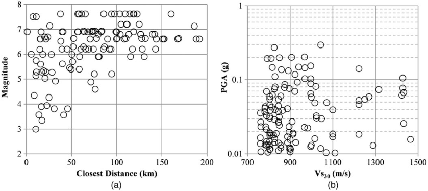
Characteristics of ground motions used in the first site response analysis database.

We developed nine sites for the site response analyses. Sites C1, C2, and C3 have V_S30 = 441 m/s (i.e., NEHRP C); sites D1, D2, and D3 have V_S30 = 263 m/s (i.e., NEHRP D); and sites E1, E2, and E3 have V_S30 = 148 m/s (i.e., NEHRP E). We calculated the shear wave velocity (V_S) profiles for each site to depths of 30 m using the correlations developed by Carlton and Tokimatsu (2014) for generic sites. For the D and E sites, we added 4 m of soil that increase in V_S with depth to give about the same impedance contrast at the soil/rock interface for all sites. This was done to simplify the investigation and make it easier to analyze the effect of the other parameters. We modeled the underlying rock layer as an elastic half-space with V_S = 760 m/s, unit weight of 23 kN/m³, and damping ratio of 1% for all nine sites. Figure 2 shows the shear wave velocity profiles, overconsolidation ratio (OCR), and unit weight with depth for each of the sites. The unit weights and OCR values were the same for all nine sites.

Figure 2.

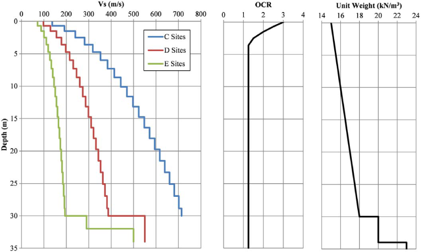
Site characteristics used in the first site response analysis database.

We calculated the shear modulus reduction and damping curves for each soil layer using the model developed by Darendeli (2001), which depends on the plasticity index (PI), OCR, mean effective confining pressure (σ′_m), loading frequency (f), and number of loading cycles (N). We modeled soil layers from 0 m to 30 m at sites C1, D1, and E1 with PI = 0; sites C2, D2, and E2 with PI = 20; and sites C3, D3, and E3 with PI = 52. We selected these PI values to give a range of soil types and shear modulus reduction and damping curves. The soil layers from 30–34 m for the D and E sites we modeled with PI = 0. We set f = 1 and N = 10 for all sites and all soil layers.

Shear modulus reduction and damping curves estimated from laboratory tests often do not predict the correct soil shear strength at large shear strains (Stewart et al. 2008). Therefore, we adjusted the shear modulus reduction and damping curves of all soil layers to match their respective shear strengths at large shear strains following the procedure outlined in Yee et al. (2013). We estimated the shear strength of the soils with PI > 0 using the SHANSEP method proposed by Ladd and Foott (1974), and assuming a shear strength ratio for normally consolidated soils of (Su/σ′_v) _NC = 0.25 and OCR coefficient of m = 0.8. We estimated the shear strength of the soils with PI = 0 using Mohr Coulomb failure criteria assuming zero cohesion, a friction angle ϕ = 35° for soils above 30 m, and ϕ = 45° for soils below 30 m. We multiplied the static shear strengths by 1.1 to adjust for rate effects, cyclic softening, and progressive failure.

We conducted all ELA and NLA in the computer program DEEPSOIL (Hashash et al. 2012). Based on the recommendations of Stewart et al. (2008), we performed the site response analyses using the outcrop motions as recorded, with no deconvolution, and with an elastic half-space underlying the soil profile. We adjusted the thickness of the soil layers so that the maximum frequency propagated through the site for the NLA was 50 Hz (0.02 s). We used the same soil layer thicknesses in the ELA as the NLA.

We used the MRDF constitutive model (Phillips and Hashash 2009) and the frequency independent damping formulation in DEEPSOIL proposed by Phillips and Hashash (2009) for all of the NLA, with the shear modulus reduction and damping curves calculated from the strength adjusted Darendeli (2001) model as described above for the reference curves. DEEP-SOIL has a built-in subroutine that determines the nonlinear parameters that give the shear modulus reduction and damping curves that best match the reference curves input by the user. The matched curves are slightly different than the strength adjusted Darendeli (2001) curves. Therefore, we used the curves generated by DEEPSOIL for the NLA to define the discrete points of the shear modulus reduction and damping curves of the ELA. This ensured that both analysis types had the same dynamic soil properties. We set the strain ratio value as 0.65 for all ELA.

Second Database of Site Response Analyses

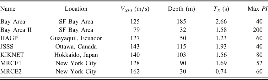
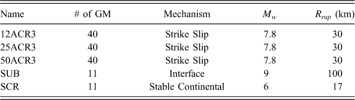
In addition to the above-mentioned database, we also included ELA and NLA from Carlton (2014). We included the results of site response analyses from seven sites, which are listed in Table 1, and five scenarios, which are listed in Table 2. The seven sites are based on actual sites with organic, high plasticity, or deep soft soil deposits (i.e., non-liquefiable NEHRP F sites) from the United States, Canada, Japan, and Ecuador. Table 2 lists the number of ground motions in each scenario, as well as the target mechanism, magnitude, and distance. Carlton (2014) selected rock ground motions with similar characteristics to the target values and then scaled the ground motions so that the mean and standard deviation of their response spectra matched those calculated by ground motion prediction equations. Carlton (2014) conducted the site response analyses in the program DEEPSOIL using a similar methodology as outlined above.

Table 1

Sites from Carlton (2014) used in the second site response analysis database

Name	Location	V_S30 (m/s)	Depth (m)	T_S (s)	Max PI
Bay Area	SF Bay Area	125	185	2.66	40
Bay Area II	SF Bay Area	79	32	1.58	200
HAGP	Guayaquil, Ecuador	127	50	1.23	60
JSSS	Ottawa, Canada	143	115	1.93	40
KIKNET	Hokkaido, Japan	140	103	1.56	80
MRCE1	New York City	128	90	1.69	52
MRCE2	New York City	162	30	0.74	60

Table 2

Ground motion scenarios from Carlton (2014) used in the second site response analysis database

Name	# of GM	Mechanism	M _w	R_rup (km)
12ACR3	40	Strike Slip	7.8	30
25ACR3	40	Strike Slip	7.8	30
50ACR3	40	Strike Slip	7.8	30
SUB	11	Interface	9	100
SCR	11	Stable Continental	6	17

Best Predictor Variable of the Difference between Ela and Nla

We calculated the difference (δ) between the predicted results of the two analysis methods as:

δ = l n (Y_{E L A}) - l n (Y_{N L A})

(1)

where Y_ELA is the output value predicted by the ELA and Y_NLA is the output value predicted by the NLA. We compared the δ values found in this study with standard deviations calculated from ground motion prediction equations (GMPEs) for similar parameters. We measure the difference δ in natural log units because most GMPEs calculate their standard deviations in natural log units. In addition, by calculating δ in natural log units it is a ratio, which makes it easier to compare the difference at large and small values of a given parameter.

We calculated the Pearson product-moment correlation coefficient ρ between the value of δ for 6 output parameters (Y) and 14 input parameters (X) to determine which input parameter was the best predictor of δ for each output parameter. Table 3 describes the 6 output and 14 input parameters. In addition, we calculated ρ between the RMSE_S and the 15 input parameters, where RMSE_S is the root mean squared error of the spectral accelerations calculated at the surface using 75 periods between and including the periods of 0.05 s and 5 s of the ELA and NLA.

Table 3

Description of the input and output parameters used to estimate the best predictor of difference between ELA and NLA

Parameter	Description
Output
PGA _S	Peak ground acceleration of the surface motion
PGV _S	Peak ground velocity of the surface motion
PGD _S	Peak ground displacement of the surface motion
I _aS	Arias intensity of the surface motion
D _5-75,S	Duration between when 5% and 75% of the Arias intensity is reached for the surface motion
T _mS	Mean period of the surface motion
Input
PGA _R	Peak ground acceleration of the input rock motion
PGV _R	Peak ground velocity of the input rock motion
PGD _R	Peak ground displacement of the input rock motion
I _aR	Arias intensity of the input rock motion
D _5-75,R	Duration between when 5% and 75% of the Arias intensity is reached for the input rock motion
T _mR	Mean period of the input rock motion
V _S30	Time average shear wave velocity of the top 30 m
T _S	Elastic site period; calculated as 4 H/V_Savg, where H is the soil profile thickness and V_Savg the average shear wave velocity of the soil profile
γ_0.5	Average shear strain when G/G_max = 0.5 for the soil layers of the top 30 m
D _min	Average minimum damping for the soil layers of the top 30 m
D _0.1	Average damping when shear strain = 0.1% for the soil layers of the top 30 m
(τ/σ'v)_max,ELA	The maximum value of the shear stress divided by vertical effective stress occurring at any depth in the ELA
PGA _{max, ELA}	Maximum PGA occurring at any depth in the ELA
γ_{max, ELA}	Maximum shear strain occurring at any depth in the ELA

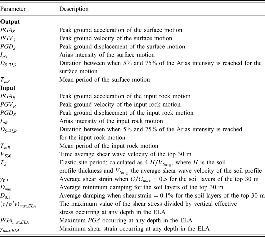
Table 4 lists the absolute values of ρ calculated between the 14 input parameters and the seven output parameters. The values in Table 4 are the larger absolute value of ρ calculated using both the arithmetic and natural log value of the input parameters. The value in parentheses next to each ρ value is the rank, where 1 signifies that the input parameter is the best predictor of δ or RMSE_S for the corresponding output parameter, and 14 is the worst. Table 4 shows that γ_max,ELA is the best predictor of δ for PGA_S, PGV_S, I_aS, and D_5–75,S, as well as the best predictor of RMSE_S. These results agree with those of Kaklamanos et al. (2013), who found that γ_max,ELA was the best predictor of the residual between observed response spectra and response spectra predicted by ELA. The shear strain is the best predictor of the difference δ between results of ELA and NLA because it directly controls the stiffness and damping values used in the analyses. Other parameters such as PGA_R or V_S30 are good predictors because they are correlated with γ_max,ELA, however, individually they are not as good of predictors as γ_max,ELA. In this paper we use γ_max,ELA instead of γ_max,NLA because it is customary to perform ELA first, then NLA if necessary; therefore, we measure change using the results of the ELA as a baseline.

Table 4

Pearson coefficient ρ between 14 input parameters and the difference δ of six predicted output parameters and the RMSE_S, the number in parentheses is the rank, where 1 is the best predictor

Parameter	PGA _S		PGV _S		PGD _S		I _aS		D _5-75,S		T _mS		RMSE
PGA _R	0.61	(2)	0.41	(2)	0.03	(14)	0.22	(4)	0.46	(2^a)	0.22	(7)	0.63	(2)
PGV _R	0.50	(6)	0.27	(8^a)	0.26	(5)	0.36	(2^a)	0.31	(7)	0.20	(8)	0.59	(5)
PGD _R	0.34	(9)	0.14	(13^a)	0.34	(2)	0.22	(5^a)	0.19	(9^a)	0.22	(6)	0.43	(9^a)
I _aR	0.55	(4)	0.33	(5)	0.08	(13)	0.15	(13)	0.37	(5)	0.31	(4^a)	0.60	(3)
D _5-75,R	0.08	(13)	0.15	(12)	0.26	(4)	0.21	(7)	0.17	(11)	0.24	(5)	0.04	(14)
T _mR	0.03	(14^a)	0.08	(14^a)	0.42	(1)	0.16	(12)	0.11	(12)	0.08	(13^a)	0.09	(13)
V _S30	0.52	(5)	0.37	(3)	0.19	(8)	0.17	(10)	0.38	(4^a)	0.35	(1^a)	0.59	(4)
T _S	0.48	(8)	0.31	(6)	0.21	(7)	0.11	(14)	0.34	(6)	0.35	(2)	0.55	(7)
γ_0.5	0.20	(12)	0.18	(10)	0.25	(6)	0.18	(8)	0.10	(13^a)	0.10	(12)	0.22	(11)
D _min	0.25	(11^a)	0.21	(9^a)	0.13	(11^a)	0.23	(3^a)	0.07	(14^a)	0.07	(14)	0.17	(12^a)
D 0.1	0.26	(10)	0.17	(11)	0.28	(3^a)	0.17	(9)	0.17	(10)	0.15	(10^a)	0.35	(10)
(τ/σ‘_v)_max	0.49	(7)	0.29	(7)	0.18	(10^a)	0.16	(11)	0.28	(8)	0.14	(11)	0.47	(8)
PGA _max	0.59	(3)	0.37	(4)	0.09	(12^a)	0.21	(6)	0.42	(3^a)	0.16	(9)	0.58	(6)
γ_max	0.73	(1)	0.55	(1^a)	0.19	(9)	0.56	(1^a)	0.53	(1)	0.33	(3)	0.81	(1)

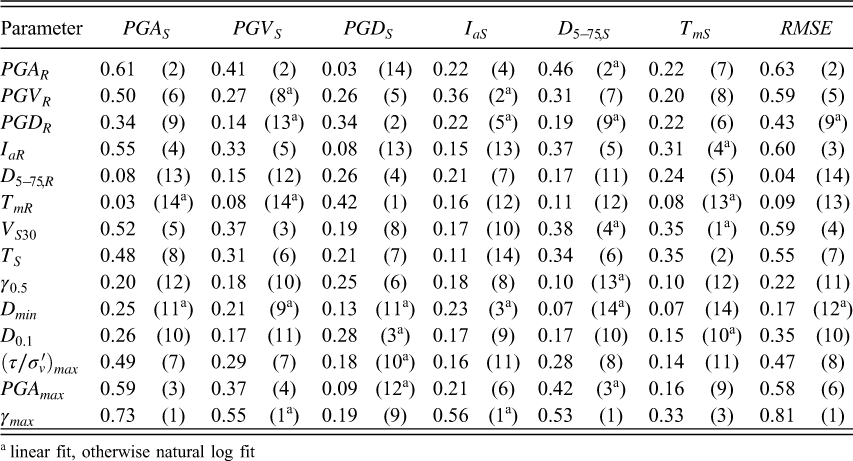
linear fit, otherwise natural log fit

Model to Predict Maximum Shear Strain

The previous section showed that γ_max,ELA is the best predictor of the difference between ELA and NLA of the 14 parameters investigated in this study. This section describes the development of a model to estimate γ_max,ELA that will aid engineers in the decision of which analysis type to perform. Assimaki and Li (2012) and Kim et al. (2013) developed models to estimate the difference between the response spectral values predicted by linear and nonlinear analyses, and equivalent linear and nonlinear analyses, respectively. The advantage of developing a model for γ_max is that it can be used to predict the difference for multiple ground motion parameters instead of only spectral acceleration values.

For shear waves in an unbounded homogeneous medium the shear strains are directly proportional to the particle velocity at all times. As a result, the shear strain time series of an earthquake can be calculated as the velocity time series divided by the shear wave velocity. The maximum shear strain can then be estimated as (Tokimatsu et al. 1989):

γ_{\max, 0} = \frac{α \times P G V_{\max}}{V_{S_{0}}}

(2)

where γ_max,0 is the initial maximum shear strain over the entire soil profile, V_S0 and PGV_max are the initial shear wave velocity and peak velocity of the layer with γ_max,0, and Tokimatsu et al. (1989) found α = 0.6. The values of V_S0 and PGV_max, however, are not known before conducting a site response analysis. Therefore, we used V_S30 instead of V_S0 and PGV_R instead of PGV_max, which gives:

γ_{\max, 0} = \frac{α \times P G V_{R}}{V_{S_{30}}}

(3)

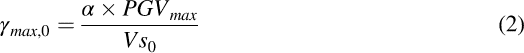
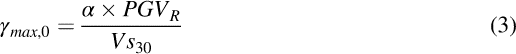
We used V_S30 as a proxy for V_S0 because it is an average value of the shear wave velocity over the soil layers most likely to experience the maximum shear strain and it is widely available for most sites. We investigated using the shear wave velocities averaged over the top 20 m (V_S20) and the top 10 m (V_S10) instead of V_S30, however, these did not improve the fit. We used PGV_R instead of PGV_max because they are highly correlated.

We used a mixed-effects regression model (Pinheiro and Bates 2000) with Equation 3 to solve for α. Mixed-effects regression is a maximum likelihood method that accounts for correlations in the data within specified groups. The total residual (δ_Total) is composed of two parts: the between-group residual (δB) and the within-group residual (δW), where δB is the mean value of the residuals for a specific group, and δW is the observed value minus δB and the predicted value. The within-group and between-group residuals are assumed to be independent normally distributed with standard deviation ϕ and τ, respectively. The total standard deviation (σ_T) for the model is then computed as σ_T = (ϕ² + τ²)^0.5. In this paper, we group the data by site, similar to Kaklamanos et al. (2013, 2015). In addition, using a mixed-effects regression allows the influence of site effects (between-group) and ground motion effects (within-group) to be more easily observed.

When we examined the residuals from Equation 3, we found a strong dependence of δW on T_mR and of δB on T_s. Figure 3a and Figure 3b show this dependence. This occurs because PGV_max is not completely described by PGV_R, but also depends on other site and ground motion parameters. When we include the effects of T_mR and T_s, the equation for γ_max,0 becomes:

γ_{\max, 0} = \frac{α \times P G V_{R} \times T_{s}}{V_{S_{30}} \times T m_{R}^{0.5}}

(4)

Figure 3.

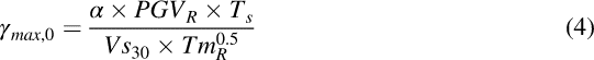
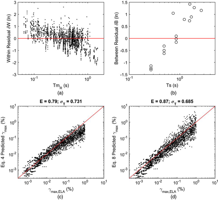
(a) Within residual and (b) between residual for Equation 3; (c) maximum shear strain calculated by equivalent linear analyses versus the maximum shear strain predicted by Equation 4, which does not account for V_S degradation, and (d) Equation 8, which does account for V_S degradation.

Figure 3c plots the predicted values using Equation 4 versus the calculated γ_max,ELA values. Figure 3c shows that at large shear strain values Equation 4 under predicts the value of γ_max,ELA. This is because at large shear strains, V_S decreases due to degradation of the soil matrix. Therefore, to calculate the maximum shear strain at large shear strains (γ_max), the degraded shear wave velocity (V_{S deg}) should be used instead of V_S0:

γ_{\max} = \frac{α \times P G V_{R} \times T_{s}}{V_{S_{\deg}} \times T m_{R}^{0.5}}

(5)

The reduction of stiffness with shear strain can be modeled using the hyperbolic model (Konder and Zelasko 1963):

\frac{G_{\deg}}{G_{0}} = \frac{1}{1 + \frac{γ}{γ_{r e f}}}

(6)

where G₀ is the initial shear modulus; G_deg is the degraded shear modulus at shear strain γ; and γ_ref is the shear strain when G/G₀ = 0.5. If we replace G₀ and G_deg in Equation 6 with V_S0 and V_{S deg} using the relation

G = d \times V_{S}^{2}

where d is the soil density, γ with γ_max, and solve for V_{S deg} we get:

V s_{\deg} = \frac{V s_{0}}{\sqrt{1 + \frac{γ_{\max}}{γ_{r e f}}}}

(7)

By combining Equations 4, 5, and 7 (assuming V_S0 = V_S30), we can solve for γ_max by using the positive solution of the quadratic equation, which gives:

γ_{\max} = γ_{\max, 0} [\frac{γ_{\max, 0}}{2 \times γ_{r e f}} + \sqrt{1 + {(\frac{γ_{\max, 0}}{2 \times γ_{r e f}})}^{2}}]

(8)

where γ_max, γ_max,0, and γ_ref are in m/m.

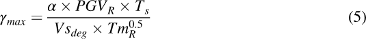
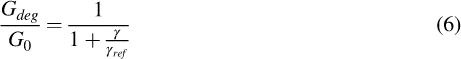
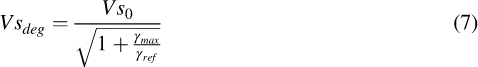
We performed mixed effects regression using Equations 4 and 8 and calculated α = 0.71. This value is similar to the value of 0.6 found by Tokimatsu et al. (1989). In Equation 8 we defined γ_ref as γ_0.5, which is the average value of γ when G/G₀ = 0.5 over the top 30 m of the soil profile. We found that the average value of γ_0.5 gave a better fit than the maximum or the minimum value. Figure 3d plots the γ_max,ELA values versus the predicted values for Equation 8. Figure 3d shows that by including the effect of V_S degradation the model is able to predict γ_max,ELA values at large shear strains better than when it does not include the effects of V_S degradation (Figure 3c). The total standard deviation is σ_T = 0.685 natural log units, or slightly less than a factor of two, and the coefficient of efficiency, E, is 0.87.

Comparison of the Difference between Ela and Nla

In this section, we present the differences δ between ground motion parameters calculated from the results of ELA with those from NLA. The previous sections showed that γ_max is the best predictor of δ, therefore, Figure 4 presents δ values versus γ_max,ELA. In Figure 4 the black dots are the individual differences, and the solid red line in each plot is calculated using the loess function (Cleveland and Devlin 1988). The loess function is a locally weighted polynomial regression line calculated at each point using a specified number of closest data points. The loess function provides an estimate of the general trend of the data. We compare the δ values found in this study with standard deviations from established ground motion prediction equations (GMPEs) to better understand the relative importance of the difference. We define the difference as non-negligible (δ_nn) when the trend line predicted by the loess function is greater than one quarter the value of the total standard deviation for a GMPE of the same parameter. The shear strain where δ_nn occurs is called the non-negligible threshold shear strain (γ_nn). We also show the mean and one standard deviation bars of the δ values for 10 bins equally spaced on a log scale.

Figure 4.

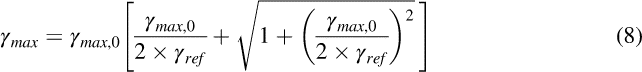
Differences δ for (a) γ_max, (b) RMSE_S, (c) PGA_S, (d) PGV_S, (e) PGD_S, (f) I_aS, (g) D_5–75,S, and (h) T_mS versus γ_max,ELA, where the black dots are the individual differences, the red lines are the trend lines predicted by the loess function, and the circles and error bars give the mean and standard deviation of the data for ten equally spaced bins.

Figure 4 shows that as γ_max,ELA increases, ELA in general predict smaller γ_max and D_5–75 values (negative loess line), larger PGA_S, PGV_S, I_aS, and T_mS values (positive loess line), and similar PGD_S values as NLA. ELA use one value of stiffness and one value of damping for each soil layer for the entire duration of the ground motion. The value of the stiffness and damping correspond to an effective shear strain that is a fraction of the maximum shear strain. As a result, the equivalent linear transfer function will use a lower stiffness and higher damping for parts of the ground motion with strains smaller than the effective shear strain, and higher stiffness and lower damping for parts of the ground motion with shear strains larger than the effective shear strain.

Because ELA over predict the stiffness for shear strains larger than the effective shear strain, they will estimate smaller maximum shear strains than NLA. For example, when the same external force is applied to a stiff object such as a rod of metal, it will deform less than a ductile object such as a rod of rubber. Earlier in this paper we developed a model for γ_max,ELA and calculated a standard deviation of 0.685 ln units, which gives δ_nn = 0.17 (0.685/4 = 0.17) and γ_nn = 0.136%. In other words, the absolute δ values of γ_max predicted by the loess line are non-negligible for γ_max,ELA values of 0.136% and larger.

As γ_max,ELA increases, Figure 4 shows that the RMSE_S values increase as well. The RMSE_S values increase as the shear strain increases because the soil behaves more nonlinearly, with a greater change in the stiffness and damping properties over the duration of the ground motion. As a result, the absolute differences between the predicted acceleration response spectra of the ELA and NLA increases. Figure 4 shows this same trend for γ_max, PGA_S, PGV_S, I_aS, and D_5–75. At γ_max,ELA = 0.1% the RMSE_S values are 0.104 natural log units, and at γ_max,ELA = 1.0% the RMSE_S values are 0.22 natural log units.

Integration from acceleration to velocity and velocity to displacement tends to dilute the high frequency components of a record and augment the low frequency components (Stewart et al. 2001). As a result, PGA, PGV, and PGD are most affected by high, mid-range, and low frequency energy, respectively. Long-period seismic waves (low frequencies) sample deeper and generally stiffer layers of a site profile and have wavelengths longer than the thickness of the soft soil layers. Therefore, they are not as affected as short period seismic waves by shallow soft soil layers that typically experience the greatest nonlinear effects. As a result, Figure 4 shows that the PGA_S δ values have the greatest trend, with ELA predicting larger PGA_S values than NLA. The PGV_S δ values show the same trend, but the bias is not as large as for the PGA_S δ values. Finally, the PGD_S δ values show no trend with γ_max,ELA because they are controlled by the longest period seismic waves. ELA estimate larger PGA_S and PGV_S values than NLA because they over predict stiffness and under predict damping for shear strains greater than the effective shear strain. Abrahamson et al. (2014) calculated standard deviations for PGA and PGV of 0.6 to 0.9 and 0.6 to 0.8 natural log units, respectively. The γ_nn value for the PGA_S is 0.067%, and for the PGV_S it is 0.70%. Even though the trend line for the PGD_S δ values is zero, the standard deviations range from 0.27 to 0.71 natural log units, which are significant when compared with the standard deviations of 0.825 and 0.90 natural log units calculated by Campbell and Bozorgnia (2008) and Alavi et al. (2011). Figure 4 shows that even though there is no bias in the prediction of PGD_S between the two analysis methods, the difference in the predicted value of PGD_S could be significant.

The trend line predicted by the loess function for I_a in Figure 4 is zero at small shear strains, negative from γ_max,ELA = 0.003% to 0.1%, and positive for γ_max,ELA > 0.1%. For γ_max,ELA < 0.003% the soil behaves almost linearly so the difference between ELA and NLA is negligible. The trend for γ_max,ELA > 0.003% is due to two opposing effects. ELA over damp ground motions for shear strains less than the effective shear strain, which reduces the total energy in the ground motion. However, for shear strains larger than the effective shear strain, ELA use smaller damping than NLA, which allows more energy to propagate to the ground surface. Because the Arias intensity is defined as the sum of the squares of the acceleration values, it gives more weight to larger acceleration values. At lower acceleration values the difference between the largest and smallest squared acceleration values is not that great, so the effect of larger damping on shear strain cycles less than the effective shear strain is dominant. At higher acceleration values, however, the large acceleration values dominate the calculation of I_a. Therefore, at higher acceleration values, the effect of under damping shear strains greater than the effective shear strain dominates, and ELA predict greater values of I_a than NLA. Travasarou et al. (2003) and Foulser-Piggot and Stafford (2011) calculated standard deviations for I_a between 0.85 to 1.3 and 0.95 to 1.3 ln units, respectively. The value of γ_nn value for I_aS is therefore 0.61%.

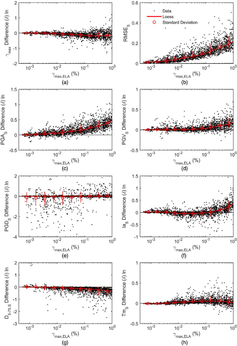
Figure 4 shows that ELA predict smaller values of D_5–75,S than NLA. This is because ELA use only one value of stiffness and damping so they under predict the accelerations at the beginning and end of a time series when the shear strain values are small, and over predict the acceleration values in the middle of the time series when the shear strain values are large. This causes the ratio of the energy to shift from the ends of the time series to the middle. This effect reduces the duration because D_5–75,S is calculated as the time between when 5% and 75% of the Arias intensity occurs. Figure 5 shows this graphically using a Husid plot for one pair of ELA and NLA. A Husid plot portrays the cumulative fraction of the Arias intensity that has occurred versus time. Figure 5 shows that the ELA have a steeper curve than the NLA, which means that more of the energy of the ground motion occurs in a shorter time span. The NLA calculate that the energy is more distributed in time, and thus predict a longer duration. Kempton and Stewart (2006) and Ghanat (2011) calculated standard deviation values for D_5–75 of 0.53 and 0.56 ln units, respectively. Therefore, the γ_nn value for D_5–75,S is 0.124%.

Figure 5.

Husid plot showing the difference in the distribution of energy and duration (D_5–75) between equivalent linear (ELA) and nonlinear analyses (NLA).

Figure 4 shows that the trend line predicted by the loess function for the T_mS δ values is positive, which means that the ELA predict larger T_mS values than the NLA. The mean period as defined by Rathje et al. (2004) is the period corresponding to the centroid of the Fourier amplitude spectrum. This study found that ELA tend to predict more peaked response spectra than NLA, with larger amplifications near the natural site period. This change in the ratio of short period to long period amplitudes relative to those predicted by NLA is why ELA predict larger values of T_mS than NLA. This phenomenon is explained in more detail later. Rathje et al. (2004) calculated standard deviations for T_m of 0.35 for NEHRP D sites and 0.49 for NEHRP C sites. The maximum absolute value of the trend line for the T_mS δ values is 0.054, which is less than 25% of 0.35. Therefore, we conclude that the difference in the predicted T_mS values between the two analysis methods is negligible.

Table 5 summarizes the non-negligible threshold differences (δ_nn), the shear strains where δ_nn occurs (γ_nn), and the largest absolute values of the loess predicted trend line (δ_max) up to a shear strain of 1% for the parameters discussed above. PGA_S has the smallest value of γ_nn at 0.039%, with the other values ranging from 0.124% to 0.700%.

Table 5

Results of the site response analysis comparison, where δ_nn is the δ value defined as the non-negligible threshold, γ_nn is the shear strain where δ_nn occurs, and δ_max is the largest absolute value of δ for γ_{max, ELA} < 1%

Parameter	δ_nn	γ_nn	δ_max
γ_max	0.171	0.136	0.185
PGA _S	0.125	0.039	0.472
PGV _S	0.150	0.700	0.183
PGD _S	0.206		0.009
I _aS	0.210	0.610	0.363
D _5-75,S	0.133	0.124	0.325
T _mS	0.088		0.054

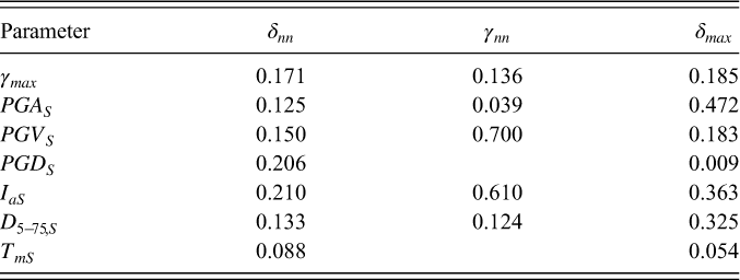
Figure 6 shows trend lines predicted by the loess function for the δ values of spectral acceleration versus period and γ_max,ELA. Figure 6 shows that at large shear strains the ELA predict larger spectral acceleration values than the NLA at short periods and periods near the natural site period, which agrees with the results of Rathje and Kottke (2011). For periods longer than 2 s, Figure 6 shows that the spectral acceleration difference is less than 0.05 natural log units. There is little difference at long periods because, as mentioned earlier, long period seismic waves are not as affected as short period seismic waves by shallow soft soil layers that usually experience the greatest nonlinear effects. These results are similar to Kaklamanos et al. (2013) and Kim et al. (2013), who found negligible nonlinear effects for periods longer than 0.5 s and 1 s, respectively. The reason for the difference in period where nonlinear effects become negligible is most likely due to the difference in the natural site periods of the sites investigated and the level of ground motion intensity. Deeper and softer soil sites have longer natural site periods that may show nonlinear effects at long periods, especially for larger intensity motions that induce larger maximum shear strains.

Figure 6.

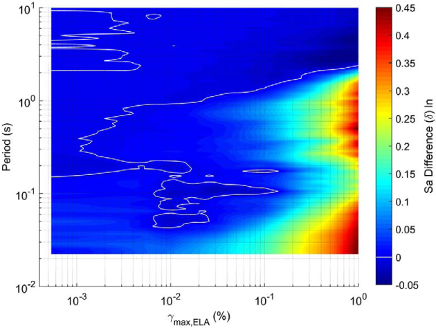
Sa δ values predicted by the loess trend line by period and γ_{max, ELA}, white line shows the zero contour.

Figure 6 also shows that for periods between 0.1 s and 0.2 s and γ_max,ELA values less than 0.1% the ELA predict similar or smaller spectral acceleration values than NLA, which agrees with the results of Rathje and Kottke (2011) and Kaklamanos et al. (2015). For γ_max,ELA > 0.1% and periods between 0.1 s and 0.2 s Figure 6 shows the opposite trend, with ELA predicting larger spectral accelerations than NLA. There is very little energy in ground motions at periods less than the peak period of the response spectrum, so a single degree of freedom oscillator follows the response of the ground more than its own natural period (Carlton and Abrahamson 2014). The response at short periods is therefore controlled by the dominant period of the acceleration time series more than the response at its own period, where the dominant period is manifested as the peak period of the response spectrum. Because ELA over predict the response spectrum near the natural site period, they predict a higher response spectral value at the peak period, which increases the response of all of the spectral acceleration values at shorter periods. At large shear strains this effect is greater than the over damping of ELA and the amplification of NLA due to stress reversals explained earlier. As a result, ELA may predict larger values of spectral acceleration than NLA for periods between 0.1 s and 0.2 s.

Figure 7 shows the combination of these effects graphically. Figure 7a shows the mean surface response spectrum of the 40 ground motions for scenario 50ACR3 at site HAGP, and Figure 7b shows the mean surface response spectra divided by their peak response spectral values. Figure 7a shows that the ELA predict larger absolute spectral accelerations than NLA for periods less than the peak period, which contradicts the findings of Rathje and Kottke (2011). However, Figure 7b, which plots the response spectra normalized by their peak values, shows that the NLA predict a broader response spectrum with larger relative Sa values for periods less than the peak period than ELA. This is why NLA predict slightly smaller Tm values than ELA. The results shown in Figure 7 are similar to a majority of the sites investigated, however, there is much variance in the results, as show in Figure 8.

Figure 7.

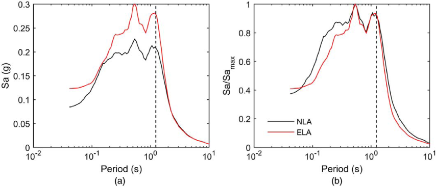
Comparison of the (a) mean response spectrum and (b) normalized mean response spectrum for the 40 ground motions in scenario 50ACR3 at site HAGP predicted at the soil surface by equivalent linear (ELA) and nonlinear analyses (NLA), dotted vertical line is the elastic site period (T_S = 1.23 s).

Figure 8.

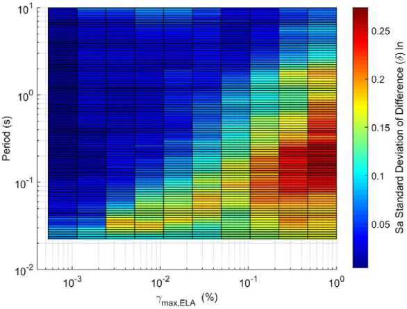
Standard deviation of Sa δ by period and γ_max,ELA.

Figure 8 shows the standard deviations of the δ values of spectral acceleration by period and γ_max,ELA for the same bins as shown in Figure 4. The trend lines shown in Figure 4 give the bias between ELA and NLA, whereas the standard deviations of the δ values show the uncertainty in that bias. The largest standard deviations in Figure 8 are for periods between 0.1 s and 0.2 s with γ_max,ELA > 0.1%. This shows that even though the loess predicted trend line is positive for these periods and shear strains, the uncertainty and scatter of the Sa δ values is large. This is further confirmed by the fact that the largest standard deviations are 0.27 natural log units, which are greater than the 0.20 to 0.25 natural log units of the trend lines shown in Figure 6.

Figure 8 also shows that as γ_max,ELA increases the standard deviations of the Sa δ values increase, with long periods showing the smallest standard deviations. The standard deviations of δ increase as γ_max,ELA increases because at larger shear strain values the difference in stiffness and damping values over the duration of the ground motion increases, which leads to greater variation in the difference between the two analysis methods. The standard deviations are smallest for long periods because, as mentioned earlier, long periods are not as affected by soil nonlinearity as short periods, therefore, the difference in the predicted results between the two analysis methods is smaller and the variation in that difference is reduced.

The standard deviations of Sa values predicted by the NGA-West2 GMPEs are between 0.5 and 0.8 natural log units, with larger standard deviations at longer periods, greater distances, and smaller magnitudes (Gregor et al. 2014). Figure 9 shows the γ_max,ELA value for each period where the Sa δ values from Figure 6 are greater than 0.125 natural log units, which we define as the non-negligible threshold. Figure 9 shows that the Sa δ values are non-negligible at γ_max,ELA values of 0.05%, 0.5%, 0.2%, and 1.0% for periods of 0.3 s, 0.1 s to 0.2 s, periods near the natural site period, and 2 s, respectively. These shear strain values are similar to those found by Kaklamanos et al. (2013, 2015) for predictions compared with measured vertical array data.

Figure 9.

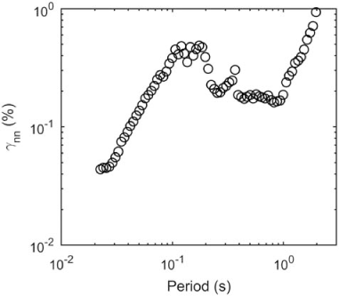
The value of γ_max,ELA when the trend line predicted by the loess function for the Sa δ values is non-negligible (γ_nn; i.e., the γ_max,ELA value when the Sa δ > 0.125 natural log units).

Summary and Conclusions

We conducted ELA and NLA in the program DEEPSOIL using 189 ground motions, nine hypothetical sites, and seven actual sites. Six of the seven actual sites contain organic, high plasticity, or deep soft soil deposits. These types of sites are the ones most likely to require a site response analysis and to generate large shear strains, therefore it is crucial that these sites be included in comparison analyses. We also corrected the shear modulus reduction and damping curves of the ELA and NLA site models to account for soil shear strength at large shear strains. If this modification is not performed, site response analyses could give erroneous results at large shear strains.

We investigated when the two methods predict different results and the magnitude of the difference (δ). We found that the best predictor of δ was the maximum shear strain (γ_max,ELA) induced in the soil column in ELA. To help engineers decide when to use ELA or NLA we developed a model to estimate γ_max,ELA values. The model predicts that as PGV_R or T_S increase, γ_max,ELA increases, and as V_S30, T_mR, or γ_0.5 increase, γ_max,ELA decreases. The advantage of developing a model for γ_max,ELA instead of directly for δ is that it can be used to predict the difference for multiple ground motion parameters. All of the input parameters necessary for the model are site and ground motion parameters, therefore the value of γ_max,ELA and the difference between results of ELA and NLA can be estimated before performing a site response analysis.

The results of the comparison between ELA and NLA show that as γ_max,ELA increases, ELA in general predict smaller γ_max and D_5–75 values, larger PGA_S, PGV_S, I_aS, and T_mS values, and similar PGD_S values as NLA. In addition, as γ_max,ELA increases, ELA predict larger spectral accelerations than NLA for periods less than 0.1 s and periods near the natural site periods of the sites investigated (0.2 < T < 2.0 s). For periods between 0.1 s and 0.2 s ELA predict similar or slightly larger spectral accelerations than NLA, and for periods greater than 2 s the differences are negligible.

We compared the δ values found in this study with standard deviations calculated from GMPEs for similar parameters. We define the difference as non-negligible when the trend of the δ values calculated by the loess function is greater than one quarter of the standard deviation calculated by a GMPE for the same parameter. Using this method, we can objectively evaluate the magnitude of the differences between the results predicted by ELA and NLA. We found that the differences between the predicted values of PGD_S and T_mS are negligible for γ_max values up to 1%, and that the differences for the other investigated parameters are non-negligible for γ_max values ranging from 0.04% to 1%. The findings of this study will allow engineers to predict what the difference will be between the results of ELA and NLA for different output parameters, and will help them decide which analysis method to use based on the needs and priorities of their specific project.

Footnotes

Acknowledgments

This first author conducted this research while supported by a Japanese Society for the Promotion of Science (JSPS) Fellowship. This support is gratefully acknowledged.

References

Abrahamson

N. A.

Silva

W. J.

and Kamai

2014. Summary of the ASK14 ground motion relation for active crustal regions, Earthquake Spectra 30, 1025–1055.

Alavi

A. H.

Gandomi

A. H.

Modaresnezhad

and Mousavi

2011. New ground-motion prediction equations using multi expression programing, Journal of Earthquake Engineering 15, 511–536.

Ancheta

T. D.

Darragh

R. B.

Stewart

J. P.

Seyhan

Silva

W. J.

Chiou

B. S. J.

Wooddell

K. E.

Graves

R. W.

Kottke

A. R.

Boore

D. M.

Kishida

and Donahue

J.L.

2014. NGA-West2 database, Earthquake Spectra 30, 989–1005.

Assimaki

and Li

2012. Site and ground motion dependent nonlinear effects in seismological model predictions, Soil Dynamics and Earthquake Engineering 32, 143–151.

Campbell

K. W.

and Bozorgnia

2008. NGA ground motion model for the geometric mean horizontal component of PGA, PGV, PGD, and 5% damped linear elastic response spectra for periods ranging from 0.01 to 10 s, Earthquake Spectra 24, 139–171.

Carlton

B. D.

and Abrahamson

N. A.

2014. Issues and approaches for implementing conditional mean spectra in practice, Bulletin of the Seismological Society of America 104, 503–512.

Carlton

B. D.

and Tokimatsu

2014. Statistical correlations for shear wave velocity of soils using limited site data, in Proceedings of the 14^th Japan Earthquake Engineering Symposium, 4–6 December 2014, Tokyo.

Carlton

B. D.

2014. An Improved Description of the Seismic Response of Sites with High Plasticity Soils, Organic Clays, and Deep Soft Soil Deposits, Ph.D. Dissertation, University of California, Berkeley.

Cleveland

W. S.

and Devlin

S. J.

1988. Locally-weighted regression: An approach to regression analysis by local fitting, Journal of the American Statistical Association 83, 596–610.

10.

Darendeli

M. B.

2001. Development of a New Family of Normalized Modulus Reduction and Material Damping Curves, Ph.D. dissertation, University of Texas, Austin.

11.

Foulser-Piggott

and Stafford

P. J.

2012. A predictive model for Arias intensity at multiple sites and consideration of spatial correlations, Earthquake Engineering and Structural Dynamics 41, 431–451.

12.

Ghanat

2011. Duration Characteristics of the Mean Horizontal Component of Shallow Crustal Earthquake Records in Active Tectonic Regions, Ph.D. Dissertation, Arizona State University, Phoenix, AZ.

13.

Gregor

Abrahamson

N. A.

Atkinson

G. M.

Boore

D. M.

Bozorgnia

Campbell

K. W.

Chiou

B. S. J.

Idriss

I. M.

Kamai

Seyhan

Silva

Stewart

J. P.

and Youngs

2014. Comparison of NGA-West2 GMPEs, Earthquake Spectra 30, 1179–1197.

14.

Hashash

Y. M. A.

Groholski

D. R.

Phillips

C. A.

Park

and Musgrove

2012. DEEP-SOIL 5.1, User Manual and Tutorial, 107 pp.

15.

Kaklamanos

Baise

L. G.

Thompson

E. M.

and Dorfmann

2015. Comparison of 1D linear, equivalent-linear, and nonlinear site response models at six KiK-net validation sites, Soil Dynamics and Earthquake Engineering 69, 207–219.

16.

Kaklamanos

Bradley

B. A.

Thompson

E. M.

and Baise

L. G.

2013. Critical parameters affecting bias and variability in site response analyses using KiK-net downhole array data, Bulletin of the Seismological Society of America 103, 1733–1749.

17.

Kempton

J. J.

and Stewart

J. P.

2006. Prediction equations for significant duration of earthquake ground motions considering site and near-source effects, Earthquake Spectra 22, 985–1013.

18.

Kim

and Hashash

Y. M. A.

2013. Site response analysis using downhole array recordings during the March 2011 Tohoku-Oki earthquake and the effect of long-duration ground motions, Earthquake Spectra 29, S37–S54.

19.

Kim

Hashash

Y. M. A.

Kottke

A. R.

Assimaki

Rathje

E. M.

Campbell

K. W.

Silva

W. J.

and Stewart

J. P.

2013. Predictive model for the relative differences between nonlinear and equivalent-linear site response analyses, Transactions from SMiRT-22, 18–23 August 2013, San Francisco, CA.

20.

Konder

R. L.

and Zelasko

J. S.

1963. A hyperbolic stress-strain formulation of sands, Proc. of 2^nd Pan American Conference on Soil Mechanics and Foundation Engineering, Sao Paulo, Brazil, 289–324.

21.

Ladd

C. C.

and Foott

1974. New design procedure for stability of soft clays, Journal of the Geotechnical Engineering Division, ASCE, 100(7), 763–786.

22.

Matasovic

and Hashash

2012. NCHRP428: Practices and Procedures for Site-Specific Evaluations of Earthquake Ground Motions (A Synthesis of Highway Practice), National Cooperative Highway Research Program, Transportation Research Board, Washington, D.C., 78 pp.

23.

Phillips

and Hashash

Y. M. A.

2009. Damping formulation for nonlinear 1D site response analyses, Soil Dynamics and Earthquake Engineering 29, 1143–1158.

24.

Pinheiro

J. C.

and Bates

D. M.

2000. Mixed Effects Models in S and S-PLUS, Springer-Verlag, New York.

25.

Rathje

E. M.

and Kottke

A. R.

2011. Relative differences between equivalent linear and nonlinear site response methods, in Proceedings of the 5^th International Conference on Earthquake Geotechnical Engineering, 10–13 January 2011, Santiago, Chile.

26.

Rathje

E. M.

Faraj

Russell

and Bray

2004. Empirical relationships for frequency content parameters of earthquake ground motions, Earthquake Spectra 20, 119–144.

27.

Snow

R. W.

2008. Comparison of Nonlinear and Equivalent Linear Site Response Analysis for Soft-Soil Sites along the Wasatch Front and Site-Specific Response Prediction for the Legacy Parkway, M.S. Thesis, University of Utah, Salt Lake City.

28.

Stewart

J. P.

Kwok

A. O.

Hashash

Y. M. A.

Matasovic

Pyke

Wang

and Yang

2008. Benchmarking of Nonlinear Geotechnical Ground Response Analysis Procedures, PEER Report 2008/04, Pacific Earthquake Engineering Research Center, University of California, Berkeley.

29.

Stewart

J. P.

Chiou

Bray

J. D.

Graves

R. W.

Somerville

P. G.

and Abrahamson

N. A.

2001. Ground Motion Evaluation Procedures for Performance-Based Design, PEER Report 2001/09, Pacific Earthquake Engineering Research Center, University of California, Berkeley.

30.

Tokimatsu

M. S.

and Yoshimi

1989. Dynamic soil properties obtained from strong motion records, Proc 12^th international conference of Soil Mechanics and Foundation Engineering 3, 2015–2018.

31.

Travasarou

Bray

J. D.

and Abrahamson

N. A.

2003. Empirical attenuation relationship for Arias intensity, Earthquake Engng Struct. Dyn 32, 1133–1155.

32.

Yee

Stewart

J. P.

and Tokimatsu

2013. Elastic and large-strain nonlinear seismic site response from analysis of vertical array recordings, J. Geotech. Geoenviron. Eng. 139, 1789–1801.