Seismic Reliability Assessment of Aging Highway Bridge Networks with Field Instrumentation Data and Correlated Failures,I: Methodology

Abstract

The state-of-the-practice in seismic network reliability assessment of highway bridges often ignores bridge failure correlations imposed by factors such as the network topology, construction methods, and present-day condition of bridges, among others. Additionally, aging bridge seismic fragilities are typically determined simply using historical estimates of deterioration parameters. This research presents a methodology to estimate bridge fragilities using spatially interpolated and updated deterioration parameters from a limited set of instrumented bridges in the network, while incorporating the impacts of overlooked correlation factors in bridge fragility estimates. Simulated samples of correlated bridge failures are used in an enhanced Monte Carlo method to assess bridge network reliability, and the impact of different correlation structures on the network reliability is discussed. The presented methodology aims to provide more realistic estimates of seismic reliability of aging transportation networks and to potentially help network stakeholders to more accurately identify critical bridges for maintenance and retrofit prioritization.

Introduction

Highway bridges are critical for the reliability of transportation networks and yet are rapidly deteriorating, with nearly one in four bridges declared as structurally deficient or functionally obsolete (ASCE 2013). Furthermore, many of these aging bridges are located in regions characterized by medium to high seismicity, spurring recent studies on the impact of aging and deterioration on seismic vulnerability (Choe et al. 2008, 2009; Ghosh and Padgett 2010, 2012). However, most of the recent seismic vulnerability estimates that account for aging mainly rely upon historical evidence of deterioration parameters available in region-specific databases or on limited laboratory test data. Such estimates may lead to potential under- or overestimation of bridge fragilities because most environmental degradation mechanisms, such as corrosion deterioration, are not static processes, but are influenced by changes in the atmosphere, such as temperature and moisture content, among others (Stewart 2004, Moncmanová 2007). Recent advances in monitoring and sensor technology have enabled field instrumentation of bridges to estimate in-situ deterioration parameters. While several researchers have demonstrated the importance of updating service load reliability using field instrumented data (Marsh and Frangopol 2008, Strauss et al. 2008, Stewart and Suo 2009), such emphasis is limited in seismic reliability predictions of highway bridges coupled with aging effects. Only recently, Huang et al. (2009) has highlighted the potential to incorporate nondestructive testing data from bridge monitoring to compute fragility estimates of reinforced concrete bridge columns. Nevertheless, the field measurement of bridges is an expensive and labor-intensive task, which makes it impractical to obtain sensor measurements of every bridge in an aging transportation network. Spatial interpolation techniques may address this issue by approximating deterioration parameters at non-instrumented bridge locations from nearby instrumented bridges in the network. While these spatial interpolation techniques have been used to predict deterioration parameters across a single bridge (Gassman and Tawhed 2004), such applications are lacking with respect to predictions across a portfolio of highway bridges distributed over a region. The interpolated or instrumented deterioration parameters can then be used to assess individual aging bridge fragilities across the network after updating the historical aging parameters using Bayesian methodologies. While updating the deterioration parameters improves upon the state-of-the-art methods to assess individual bridge fragilities and subsequently provides a more accurate estimate of the bridge network reliability, such estimates may be further enhanced by considering correlations among bridge failures.

The prevalent practice in seismic reliability studies of bridge networks assumes independent failures among bridges. However, recent research has shown that correlated failures stemming from correlations in seismic intensities result in significant changes in both network reliability and seismic loss estimates (Wesson and Perkins 2001, Kiremidjian et al. 2007, Kang et al. 2008, Jayaram and Baker 2009, Bocchini and Frangopol 2011). The failure correlations from seismic intensity are triggered by factors such as the geographical proximity of the bridges in a transportation network. Intensity correlations affect the bridge failure probabilities by an error term in computing the intensity measure at bridge locations throughout the network, as in Equation 1:

\ln (i m) = f (a r g) + ε_{\ln (i m)}

(1)

in which im is the intensity measure at the site of network bridges, arg is a vector representing the arguments of the attenuation relationship (such as the earthquake magnitude, distance to the seismogenic rupture area, and subsurface conditions), and ∊_ln( _im ₎ is a normally distributed error term with zero mean. Producing sets of network consistent intensities for a probabilistic seismic hazard analysis (PSHA) involves quantifying this error term, a task that is explored elsewhere (Wesson and Perkins 2001, Jayaram and Baker 2009, Wesson et al. 2009).

Unlike intensity correlations, the impact of bridge failure correlations originating from correlated bridge structural capacities has not received much attention. The structural vulnerabilities of bridges may be correlated due to factors such as the structural conditions of the bridges, similar construction detailing, traffic flows, fatigue, and proximity to deteriorating environments, among others (Kiremidjian et al. 2007). The impact of such sources on correlated seismic response of structures is not always known, nor have all potential sources of correlations been identified.

This research focuses on quantifying the impact of correlations that stem from bridge structural capacities under joint seismic and aging threats. Since the influence of intensity correlations has been presented elsewhere (e.g., Jayaram and Baker 2010), this study considers a single seismic scenario analysis for which the error term in Equation 1 can be set to zero (Wesson et al. 2009). The reason is that a single seismic scenario analysis does not involve the inter-event error, while the intra-event error is set to zero since the mean intensity measure value will be used in the analysis. Moreover, some of the factors affecting the structural vulnerability of bridges (such as the effects of the corrosive agents) are directly modeled in bridge fragility models. This study, therefore, is concerned with the contributing factors to the correlation structure among bridge failures, which are not integrated into bridge fragility models, and are referred to as “extra correlations” in this article.

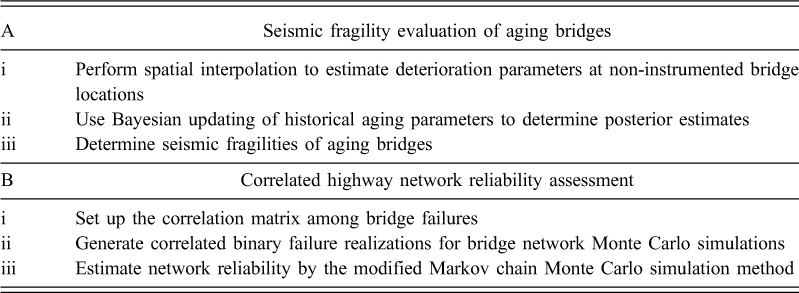
The proposed bridge reliability assessment in networks (BRAN) methodology improves upon the state-of-the-art in two ways: (1) by evaluating seismic fragilities for aging highway bridges in a network after Bayesian updating of spatially interpolated/measured deterioration parameters; and (2) by estimating the network reliability considering correlated bridge failures. This integrated methodology is summarized in Table 1 and is explained and exemplified throughout this two-part paper. Individual bridge failure probabilities are determined in Stage A by a parameterized fragility formulation approach after considering the updated statistical distributions of the deterioration parameters, while bridge network reliability is assessed in Stage B by incorporating the extra correlations among individual bridge failure probabilities. While the presented methodology is generally applicable to evaluate the bridge network reliability with correlated bridge failures, the companion Application paper proposes methods to determine the correlation values when direct estimates are not available. For this purpose, the aggregated effects of several available information sources on the level of correlations among bridge failures are examined and combined to form a correlation structure.

Table 1

The BRAN methodology to assess network reliability, including aging bridge instrumentation data and correlated bridge failures

A	Seismic fragility evaluation of aging bridges
i	Perform spatial interpolation to estimate deterioration parameters at non-instrumented bridge locations
ii	Use Bayesian updating of historical aging parameters to determine posterior estimates
iii	Determine seismic fragilities of aging bridges
B	Correlated highway network reliability assessment
i	Set up the correlation matrix among bridge failures
ii	Generate correlated binary failure realizations for bridge network Monte Carlo simulations
iii	Estimate network reliability by the modified Markov chain Monte Carlo simulation method

The following section explains spatial interpolation using Kriging and subsequent Bayesian updating of field measurable bridge deterioration parameters (Stages A.i and A.ii). This discussion leads to the development of parameterized fragility formulations to express the seismic vulnerability of aging bridges as a function of the seismic intensity and critical bridge parameters (Stage A.iii). Prior to Stage B, the impact of extra correlations on the reliability of bridge networks is discussed through closed-form network reliability calculations to emphasize their potential significance in network reliability evaluations. Stages B.i and B.ii detail the simulation of correlated bridge failures, utilizing their parameterized fragility functions and the estimated extra correlation values. The modified Markov chain Monte Carlo (MCMC) simulation method is then introduced in Stage B.iii to estimate the reliability of bridge networks based on the simulated correlated bridge failures. The final section provides a summary of the BRAN methodology and offers conclusions.

Spatial Interpolation and Bayesian Updating of Deterioration Parameters in Bridge Networks (Stages A.I and A.Ii)

Environmentally dependent deterioration parameters or degrading agents, such as chloride concentration, diffusion coefficient, corrosion rate, etc., are strongly correlated across bridges located within close proximity. Consequently, spatial interpolation techniques can be employed to assess deterioration parameters for non-instrumented highway bridges from sensor monitoring data of a limited number of instrumented bridges within the network. In the absence of instrumentation, aging bridge reliabilities are often computed using historical estimates of the degrading agents available in region-specific databases (Enright and Frangopol 1998, Ghosh and Padgett 2010) or from limited laboratory test data (Choe et al. 2008, 2009). Hence, the field-measured and interpolated deterioration parameters can be used to statistically update available probability distributions of aging parameters and make better predictions of seismic bridge fragilities. The following sections elaborate further on the spatial interpolation and statistical updating techniques of deterioration parameters.

Spatial Interpolation of Deterioration Parameters

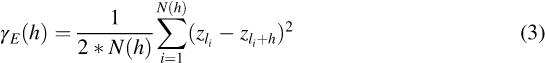
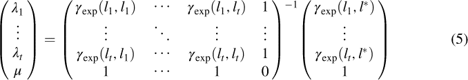
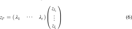
While several interpolation procedures are available in spatial data analysis, this study employs Kriging (Krige 1951), a widely popular method in the field of geostatistics. Although several strategies, such as polynomial fittings, trend surface analysis, etc., exist for spatial interpolation, Kriging has several clear advantages over these methods. First, Kriging incorporates the correlation structure among observations while making predictions at unobserved locations. Second, while such methods as trend surface analysis can be significantly affected by the location of data points and produce extreme fluctuations in predicted estimates in sparse areas, Kriging predictions are more stable over sparsely sampled regions (Mackaness and Beard 1993). However, user discretion is recommended with respect to using Kriging for spatial interpolation when localized effects or other discontinuities are present in the spatial process. Under such circumstances, the Kriging procedure is known to perform poorly and use of alternative spatial interpolation techniques, such as Bayesian partition modeling is recommended. It is assumed in this study that sudden discontinuities are rare for deterioration parameters distributed across a region, and hence, the Kriging procedure is adopted. The Kriging method belongs to the family of linear least squares estimation algorithms and helps to determine the magnitude of influence of neighboring observations when predicting values at unobserved locations (Trauth et al. 2010). Although different Kriging methods exist, the popular ordinary point Kriging method is adopted in this study, owing to its simplicity while retaining the key advantages of the Kriging procedure (Mount et al. 2008, Trauth et al. 2010). While details of this method can be found elsewhere (Cressie 1993, Olea 1999), the main steps involved in this procedure are provided in the context of inferring deterioration parameters across a bridge network.

Step 1: Construct an experimental variogram (called semivariance), which provides an estimate of the squared difference between instrumented values of deterioration parameters relative to their separation distances of the respective monitored bridge locations, as follows:

γ (h) = 0.5 {(z_{l} - z_{l + h})}^{2}

(2)

where γ(h) is the semivariance, and z_l and z_l₊ _h are the instrumented deterioration parameter values at bridge location l and another location separated by distance h (also called “lag interval”) from l.

Step 2: Derive a variogram estimator, γ_E(h), which summarizes the central tendency of observations at different instrumented bridge locations. The form of the variogram estimator is typically given by:

γ_{E} (h) = \frac{1}{2 * N (h)} \sum_{i = 1}^{N (h)} {(z_{l_{i}} - z_{l_{i} + h})}^{2}

(3)

where N(h) is the number of pairs within the lag interval h. Next, a parametric curve called the variogram model is fitted to approximate the variogram estimator with the most appropriate mathematical representation. Due to theoretical constraints, only functions satisfying certain mathematical characteristics can be used as variogram models. The most prevalently used variogram models include the spherical model, exponential model, and linear models (Trauth et al. 2010). Following the goodness-of-fit test results corresponding to these traditionally adopted variogram models, the exponential model with nugget effect is employed in this study. The form of this exponential variogram model is given as:

γ_{\exp} = n_{g} + s (1 - e^{\frac{- 3 h}{a}})

(4)

where, n_g is the nugget, s is the sill, and a is the range. In the variogram model, n_g is the intercept of the variogram and represents the sub-grid scale variations, s equals the total variance of the data set representing the value of the semivariance as lag h goes to infinity, and a controls the degree of correlation between the data points (Cressie 1993, Myers 1997, Reimann 2008).

Step 3: Use the exponential variogram model γ_exp to spatially interpolate deterioration parameters through Kriging, which uses a weighted average of neighboring point observations to estimate values at unobserved locations. The weighting points λ_i‘s required for the interpolations are computed as:

(\begin{matrix} λ_{1} \\ ⋮ \\ λ_{t} \\ μ \end{matrix}) = {(\begin{matrix} γ_{\exp} (l_{1}, l_{1}) & \dots & γ_{\exp} (l_{1}, l_{t}) & 1 \\ ⋮ & ⋱ & ⋮ & ⋮ \\ γ_{\exp} (l_{t}, l_{1}) & \dots & γ_{\exp} (l_{t}, l_{t}) & 1 \\ 1 & \dots & 1 & 0 \end{matrix})}^{- 1} (\begin{matrix} γ_{\exp} (l_{1}, l^{*}) \\ ⋮ \\ γ_{\exp} (l_{t}, l^{*}) \\ 1 \end{matrix})

(5)

where γ_exp(l_i, l_j) represents the exponential variogram estimate between the points l_i and l_j, l* is the non-instrumented bridge location where the interpolation estimates of deterioration parameters are desired, t is the total number of instrumented bridge locations, and μ is the Lagrange multiplier used to minimize the Kriging error and satisfy the unbiasedness condition ∑ _i ₌₁ⁿ λ_i = 1. Computation of λ_i‘s is followed by estimation of the deterioration parameter z_l* at location l* from Equation 6. It is noted that z_l_* denotes the mean of the Kriging estimate for the deterioration parameter at the interpolated non-instrumented bridge location.

z_{l *} = (\begin{matrix} λ_{1} & \dots & λ_{t} \end{matrix}) (\begin{matrix} z_{l_{1}} \\ ⋮ \\ z_{l_{t}} \end{matrix})

(6)

Although not considered in this study, the uncertainty associated with this interpolated estimate can also be quantified using the Kriging variance. The variability about the mean estimate is captured to a certain extent in this study by repeating the Kriging procedure for many samples from the parent distribution of the deterioration parameters at the instrumented bridge locations. While this is demonstrated in the Application paper, it is acknowledged herein that in a strict sense, the Kriging variance should also be incorporated within the proposed framework. Repeating the above steps for all non-instrumented bridge locations l^*, the Kriging methodology helps to determine interpolated estimates of deterioration parameters across the network using the data from a subset of instrumented bridges. Field-measured/interpolated aging parameter estimates are used next to update the historical estimates of deterioration parameters.

Statistical Updating of Deterioration Parameters

Statistical procedures, such as the Bayesian updating method, have emerged in infrastructure engineering as a powerful tool to rationally combine the information available on deterioration parameters from historical databases and new inspection data from field measurements (Enright and Frangopol 1999, Congdon 2006, Straub and Kiureghian 2010). This updating technique preserves previously available information and systematically incorporates new field measurements of deterioration parameters. The general Bayesian updating procedure is presented in Equation 7:

p (φ | κ) = \frac{q (κ | φ) p (φ)}{\int_{- \infty}^{\infty} q (κ | φ) p (φ) d φ}

(7)

where p(ϕ|κ) is the updated posterior distribution of the deterioration parameter based on historical data and new inspection results, p(ϕ) is the prior distribution of the deterioration parameter ϕ ∈ Φ based on historical records from region specific databases (for instance, Federal Highway Administration reports), and q(κ| ϕ) is the likelihood function in which κ ∈ K is a random variable representing a new deterioration parameter information from field instrumentation data or spatial interpolation. The posterior updated probability density functions are then used to determine the extent of structural deterioration of bridge components corresponding to each bridge in the network. Such deterioration-affected structural parameters inform the upcoming parameterized fragility formulations of aging highway bridges.

Parameterized Seismic Fragility Formulation for Aging Bridges (Stage A.Iii)

The vulnerability of highway bridges under seismic shaking can be conveyed through seismic fragility curves. These conditional probabilistic statements were traditionally developed to predict the probability of meeting or exceeding a particular damage state of a bridge component or system given the intensity of ground motions (im), as shown in Equation 8:

F r a g i l i t y = P [D e m a n d > C a p a c i t y | i m]

(8)

A major disadvantage of such single-parameter fragility curves lies in their inability to assess the impact of any deteriorating bridge component on bridge performance during earthquakes, or to incorporate new information on deterioration parameters without the need for costly re-analysis. Hence, these single-parameter fragility curves can only be used to represent the seismic vulnerability of a non-deteriorating bridge or a bridge with an assumed level of deterioration using historical estimates.

Many researchers have recently demonstrated the importance of considering deterioration of critical bridge components such as reinforced concrete (RC) columns and bridge bearings for deriving aging bridge seismic fragility curves (Choe et al. 2009, Ghosh and Padgett 2010, Alipour et al. 2010, Rokneddin et al. 2011). Additionally, Nielson (2005) identified several critical bridge structural modeling parameters for a variety of bridge types within the Central and Southeastern U.S. bridges inventory. Hence, the bridge fragility models derived in Stage A.iii are conditioned on deterioration-affected structural parameters, as well as on the critical structural modeling parameters identified by Nielson (2005). Consequently, Equation 8 is modified to represent bridge fragility as:

F r a g i l i t y = P [D e m a n d > C a p a c i t y | i m, x_{1}, x_{2}, ..., x_{m}]

(9)

where x = {x₁, x₂, …, x_m}, is the set of m critical parameters affecting the seismic performance of the deteriorating bridge components and includes: (1) critical modeling parameters, and (2) parameters affected by deterioration mechanisms. Note that only field measurable parameters (using sensor devices or other practical techniques) are chosen to condition and update the fragility estimates herein. Other parameters that are critical but not field measurable are also considered in the fragility analysis, but are treated as time-invariant random variables to propagate their uncertainty when deriving the fragility models.

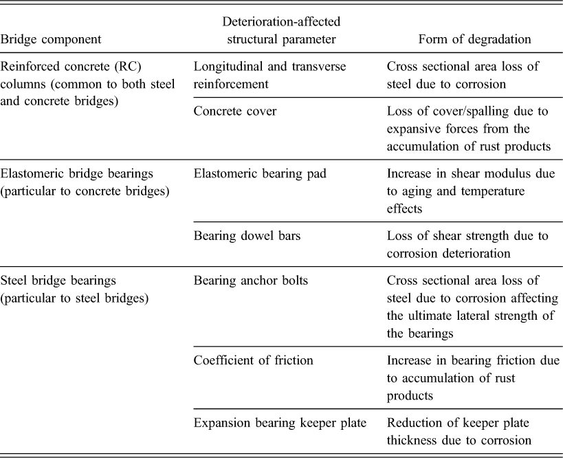
The deterioration-affected structural parameters and forms of degradation corresponding to materially different bridge types are shown in Table 2. The deterioration mechanisms associated with each form of degradation are discussed in further detail in Ghosh and Padgett (2010, 2012). The following subsections elaborate on the approach to construct the new parameterized fragility estimates using the set of conditioned parameters x .

Table 2

Deterioration-affected structural parameters and forms of degradation corresponding to different bridge types

Bridge component	Deterioration-affected structural parameter	Form of degradation
Reinforced concrete (RC) columns (common to both steel and concrete bridges)	Longitudinal and transverse reinforcement	Cross sectional area loss of steel due to corrosion
	Concrete cover	Loss of cover/spalling due to expansive forces from the accumulation of rust products
Elastomeric bridge bearings (particular to concrete bridges)	Elastomeric bearing pad	Increase in shear modulus due to aging and temperature effects
	Bearing dowel bars	Loss of shear strength due to corrosion deterioration
Steel bridge bearings (particular to steel bridges)	Bearing anchor bolts	Cross sectional area loss of steel due to corrosion affecting the ultimate lateral strength of the bearings
	Coefficient of friction	Increase in bearing friction due to accumulation of rust products
	Expansion bearing keeper plate	Reduction of keeper plate thickness due to corrosion

Phase 1: Develop Surrogate Demand Models for Component Responses Using Response Surface Methodology

The computational demands of complex three dimensional finite-element simulations of bridge models subjected to seismic shaking can be prohibitive for probabilistic analysis across a full parameter space. Hence, in order to reduce this computational burden, surrogate models or metamodels can be formulated to provide an analytically sound relationship between the predicted values (such as column curvature ductility, bearing deformation, etc.) and the predictor variables (such as earthquake intensity, reinforcing steel area, bearing pad shear modulus, etc.; Simpson et al. 2001). For the case at hand, the response y_k corresponding to the k^th bridge component (k = 1, 2, …, K, where K is the total number of bridge components) constitute the predicted values, while the predictors are the ground motion intensity (im) and the vector x . Let this joint set of im and x be represented by ψ such that ψ = {im, x}. If the true (but unknown) relationship between the predictors and the predicted variable can be represented as

y_{k} = f (ψ)

(10)

then the function g( ψ ) is said to statistically approximate this “complex and implicit” (Towashiraporn 2004) relationship f ( ψ ) as:

y_{k} = g (ψ) + ε

(11)

where ∊ is the total error resulting from lack-of-fit and is assumed to be a zero mean normal random variable.

Traditionally, development of surrogate models/metamodels from computer simulations primarily consists of three main steps as outlined in Simpson et al. (2001) and summarized here:

Choose an efficient experimental design strategy to generate a sequence of experiments (finite-element simulations) to be performed. Each experimental design run in the sequence is expressed in terms of the factors (predictor variables) set at specified levels. For instance, if the entire sequence of experiments is represented by the matrix X , then, an experimental design run will correspond to a row of X .

Conduct the three dimensional finite-element analysis simulations of bridge models to obtain the data ( y_k ) for component responses (such as column curvature ductility, bearing deformation etc.) corresponding to each experimental design run.

Choose a functional form of the surrogate model g( ψ ) and fit the surrogate model g( ψ ) to the observed data obtained in Step 2.

Pertaining to the experimental design strategy, each of the critical bridge parameters (x_i for i = 1, 2, …, m) is analyzed at five different levels to gain an in-depth understanding of the influence of the interaction between parameter levels that may be experienced throughout a bridge's lifetime on its seismic response. To overcome the curse of dimensionality, a special class of computer aided experimental design called D-Optimal design (Kiefer and Wolfowitz 1959) is adopted which is particularly useful when classical/“non-optimal” design strategies such as fractional factorial design, central composite design, etc., are impractical (Step 1 of surrogate model development). The most significant advantage of the D-Optimal design lies in its ability to maximize the amount of information generated in a limited number of runs besides being more efficient than classical design strategies in exploring the entire sample space of different parameter combinations (Kazmer 2009). This design methodology typically generates experimental designs using numerical optimization techniques and an iterative search algorithm that seeks to minimize the variance of parameter estimates (or maximize the determinant D = X^TX , with X being the design matrix of model terms reflecting the sequence of experiments; Goos and Jones 2011). In this paper, the computer aided D-Optimal design is generated using the row-exchange algorithm in MATLAB (The MathWorks 2004). After generating the experimental design matrix X , nonlinear dynamic analyses of three dimensional bridge models are conducted by pairing each experimental design run (each row of X ) with a ground motion from the synthetic ground motion suites developed by Wen and Wu (2001) and Rix and Fernandez (2004) for the Central and Southeastern United States. In this study, the ground motions are treated as an uncontrollable factor, and their uncertainty is propagated throughout the experimental design matrix by using a total of 96 different ground motions with multiple replications throughout the analysis. Future studies by the authors will further enhance the propagation of ground motion uncertainty in the experimental design by using a subset ensemble of ground motions per experimental design run. The process of generating the experimental design matrix with each row paired with an earthquake record is then followed by nonlinear dynamic time history analysis of finite-element bridge models. This corresponds to Step 2 in the framework for developing the seismic demand metamodel. The present study employs the finite-element package OpenSees for bridge modeling and nonlinear time history analyses (Mazzoni et al. 2009), using the suggestions in Nielson and DesRoches (2007) and Ghosh and Padgett (2010, 2011). The response of the k^th bridge component due to seismic shaking, such as the peak bearing deformation or column curvature ductility demand, constitutes the vector y_k in Equation 11.

In Step 3, the results obtained in the previous step are used to fit a model between each of the dependent predicted variables y_k and the predictors ψ = {im, x } using the polynomial response surface model (Box and Wilson 1951). These surrogate models have been used in studies pertaining to the reliability of structural systems and are recognized for their ability to provide a good approximation of complex finite-element simulation results, particularly when the response functions are not too nonlinear (Bucher and Bourgund 1990, Rajashekhar and Ellingwood 1993, Guan and Melchers 2001, Towashiraporn 2004). The polynomial response surface metamodel uses a multivariate function of the predictor variables to fit the predicted values using a least squares regression approach (Simpson et al. 2001). Simply put, the response surface equation is a polynomial regression approximation to the data set, and the coefficients obtained during the model-fitting process for the predictor variables im and x_i(i = 1, 2, …, m) constitute the functional form of g( ψ ). In this research, the multilinear regression model involving a constant term, linear terms, and interaction terms is adopted as the response surface metamodel (Equation 12). A preliminary study conducted by the authors revealed that inclusion of quadratic terms in the adopted second-order predictive model did not increase the goodness of fit estimates significantly. Hence, the model is restricted to interaction terms only to keep it as simple as possible. Bridge reliability estimates using this metamodel are compared with state-of-the-art fragility development procedures in the companion Application paper.

\begin{matrix} g (ψ) = β_{0} + [β_{i m} i m + β_{1} x_{1} + β_{2} x_{2} + \dots + β_{m} x_{m}] + [β_{i m, 1} i m x_{1} + β_{i m, 2} i m x_{2} + \dots \\ + β_{i m, m} i m x_{m} + β_{1, 2} x_{1} x_{2} + \dots + β_{m - 1, m} x_{m - 1} x_{m}] \end{matrix}

(12)

where β₀ is the constant coefficient, β_im, β₁, …, β_m are the linear coefficients, and β_im,1, β_im,2, …, β_m–1,m are the interaction coefficients. Consequently, regression statistics parameters, such as the adjusted R² and the mean squared error ( ∊ in Equation 11), are estimated after fitting the multilinear response surface metamodel.

Phase 2: Use the Surrogate Demand Models to Develop Bridge Fragilities via Logistic Regression

In this phase, the surrogate demand models are used to develop seismic fragility estimates. It should be noted herein that the seismic demands of the different components are correlated, and such component correlations are considered while drawing component demand samples. The component demand correlations are calculated by computing the pairwise correlations of the seismic response of bridge structural components obtained from the finite-element simulations of bridge models (Nielson and DesRoches 2007, Ghosh and Padgett 2010). These component correlations aid in the construction of the covariance matrix, which is used to establish the joint multivariate normal distribution of component demands. The individual bridge component demands are then sampled from this multivariate normal distribution to derive aging bridge fragility curves. Fragility estimates represent the probability of the demand exceeding the capacity of components or systems given a set of conditioned parameters as evident from Equation 9. Fragility curves are generated in this study via logistic regression using the Monte Carlo simulation approach. In this approach, a large number of demand samples (N_logistic) are first generated using the surrogate demand model y_k for different combinations of elements in ψ for each of the K bridge components after considering component demand correlations. Then, N_logistic component capacity estimates are generated from their distributions corresponding to a specific damage state. In this study, the component capacity distributions are adopted from Nielson and DesRoches (2007), and the damage state chosen is the extensive damage state, which results in closure of the bridge for at least a week following a seismic event (Padgett and DesRoches 2007). After generating component demand and capacity estimates, a binary vector of 0's (survival) and 1's (failures) is simulated, corresponding to whether the demand d exceeds the capacity c or not. Mathematically, the i^th Monte Carlo trial, or in other words, the i^th element of this binary vector bin_k corresponding to the k^th bridge component can be populated as:

b i n_{k, i} = {\begin{array}{l} 1 & i f & d_{k, i} \geq c_{k, i} \\ 0 & i f & d_{k, i} < c_{k, i} \end{array}

(13)

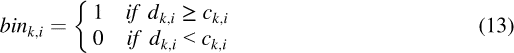
This vector of binary elements is used to develop component-level fragility curves through the logistic regression method which has been used in the past for constructing multi-dimensional fragility surfaces particularly for vector valued earthquake intensity measures (Baker and Cornell 2005, Koutsourelakis 2010). In this study, the concept of logistic regression for fragility modeling is extended to include the ground motion intensity measure and the critical and field measurable bridge parameters. In this case, bin_k represents the dependent binary variable and let the probability that bin_k_, _i = 1 given a set of parameter combinations of im, x₁, x₂, …, x_m for the i^th Monte Carlo trial be represented by p_k. Then, according to the logistic regression formulation the following equation can be derived for the k^th bridge component as:

\log i t (p_{k}) = \log (\frac{p_{k}}{1 - p_{k}}) = θ_{k, 0} + θ_{k, i m} i m + \sum_{j = 1}^{m} θ_{k, j} x_{j}

(14)

where “θ_k_,0, “θ_k_, _im and “θ_{k, j}‘s (j = 1, 2, …m) are the logistic regression coefficients corresponding to the k^th bridge component. The above equation in turn leads to the expression for p_k as:

p_{k | i m, x_{1}, x_{2}, ..., x_{m}} = P [b i n_{k, i} = 1 | i m, x_{1}, x_{2}, ..., x_{m}] = \frac{e^{θ_{k, 0} + θ_{k, m} i m + \sum_{j = 1}^{m} θ_{k, j} x_{j}}}{1 + e^{θ_{k, 0} + θ_{k, m} i m + \sum_{j = 1}^{m} θ_{k, j} x_{j}}}

(15)

Recognizing that bin_k_, _i = 1 is a statement equivalent to Demand > Capacity, it should be noted that the above equation is equivalent to Equation 9 for the fragility estimate at the component level.

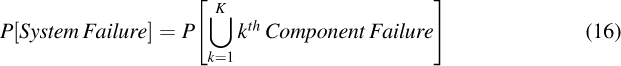
The system-level fragility estimate is obtained using the series system approximation following Nielson and DesRoches (2007) such that failure of one or more of the bridge components represents system-level failure and can be represented as:

P [S y s t e m F a i l u r e] = P [\cup_{K = 1}^{K} k^{t h} C o m p o n e n t F a i l u r e]

(16)

where K was defined earlier as the total number of bridge components. This system-level model enables the construction of a vector of binary elements (survival/failure) for the bridge system from the binary vector of each of the individual components. For instance, the binary vectors from each of the K bridge components can be arranged in matrix form as:

B I N = [\begin{array}{l} ⋮ & ⋮ & ⋮ & ⋮ \\ b i n_{1} & b i n_{2} & \dots & b i n_{K} \\ ⋮ & ⋮ & ⋮ & ⋮ \end{array}]

(17)

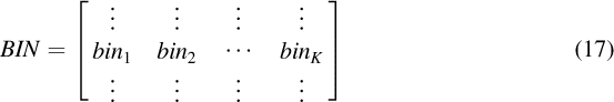
Following the series system assumption, the i^th element of the binary vector of the system (bin_sys) will equal 1 (representing failure) if at least one element in the i^th row of the matrix BIN equals 1. However, if all the elements in the i^th row are 0 (representing survival), then the i^th element of vector bin_sys is also 0. Establishing vector bin_sys is followed by fitting a logistic regression model at bridge system level as:

p_{s y s | i m, x_{1}, x_{2}, ..., x_{m}} = P [b i n_{s y s, i} = 1 | i m, x_{1,} x_{2}, ..., x_{m}] = \frac{e^{θ_{s y s, 0} + θ_{s y s, i m} i m + \sum_{j = 1}^{m} θ_{s y s, j} x_{j}}}{1 + e^{θ_{s y s, 0} + θ_{s y s, i m} i m + \sum_{j = 1}^{m} θ_{s y s, j} x_{j}}}

(18)

where “θ_sys_,0, “θ_sys_, _im , and “θ_sys_, _j ‘s are the logistic regression coefficients at the system level. The logistic regression model fitted to binary survival-failure vector at the system level helps to assess the system probability of failure conditioned on the ground motion intensity im and the parameter vector x . The impact of each of the conditioned parameters in the above equation can be assessed by considering “slices” of the multi-dimensional fragility model. Additionally, uni-dimensional bridge system seismic fragility curves conditioned only on im can be determined after integrating over the entire domain of the historically estimated or Bayesian updated probability density functions corresponding to each parameter in x (Equation 19). The elements within the parameter vector x are carefully chosen in this study such that they are statistically independent of each other (demonstrated in the Application paper). This assumption permits the multi-dimensional integration over the parameter specific distributions without the need to construct the joint distribution.

p_{s y s | i m} = \int_{x_{1}} \int_{x_{2}} \dots \int_{x_{m}} \frac{e^{θ_{s y s, 0} + θ_{s y s, i m} i m + \sum_{j = 1}^{m} θ_{s y s, j} x_{j}}}{1 + e^{θ_{s y s, 0} + θ_{s y s, i m} i m + \sum_{j = 1}^{m} θ_{s y s, j} x_{j}}} f (x_{1}) ... f (x_{m}) d x_{1} ... d x_{m}

(19)

Bridge failure probabilities are evaluated as point estimates of individual aging bridge fragility curves for corresponding seismic intensity levels and are employed to estimate the network-level reliability, that constitutes Stage B of the BRAN methodology.

Impact of Extra Correlations on Network Reliability Assessments

The reliability assessment of bridge networks integrates the evaluated bridge failure probabilities from Stage A with estimated correlations stemming from the extra correlation sources. While the subsequent sections elaborate on the steps in Stage B for network reliability evaluation, this section demonstrates the positive or negative impacts of accounting for extra correlations on network reliability estimates prior to implementing a quantitative network reliability assessment by Monte Carlo simulations.

Although other many failure criteria are available in the literature, the adopted network failure definition in this study is the failure to retain connectivity between a predefined set of origin and destination (O-D) nodes in the network, also known as connectivity reliability. The destinations nodes are typically the densely populated, critically important parts of the bridge network, which benefit from relief operations and emergency assistance, or require access. The origin nodes can be supply points or the designated regions in the network from which resources deploy. Retaining connectivity among origin and destination nodes in a seismic event is the minimum necessary condition to fulfill the objectives of a transportation network, as discussed in the literature (Chen et al. 2002, Rokneddin et al. 2011). This section demonstrates that the connectivity reliability of bridge networks depends on the bridge failure probabilities, the correlation structure among failures, and the topology of the network, which defines the paths from the origin to the destination.

To illustrate the correlation effects, first consider a network consisting of merely two nodes where both nodes must survive for the network to remain functional. The network probability of failure may be written as:

P_{f} = P (F_{1} \cup F_{2}) = P (F_{1}) +P (F_{2}) -P (F_{1} \cap F_{2})

(20)

where F₁ and F₂ denotes the failure event of nodes 1 and 2 respectively. A positive correlation between the two failure events has a favorable effect on network reliability as it results in an increase in P(F₁ ∩ F₂), and therefore, reduces the network failure probability. A negative correlation, on the other hand, increases the vulnerability of the network. Before expanding the problem, consider the following two equalities on two given events A and B:

P (\bar{A \cap B}) = 1 - P (A \cap B)

(21)

P (\bar{A \cup B}) = 1 - P (A \cup B)

(22)

It is readily inferred that a positive correlation among Events A and B increases the probability of their joint occurrence, which in turn induces a decrease in the left-hand side of Equation 21 and a decrease in the left-hand side of Equation 22 by the same amount. Now, let's consider the simple network presented in Figure 1. The network failure probability may be expressed by mutually exclusive collectively exhaustive events as in Equation 31:

P_{f} = P (F_{1} \cup F_{4}) + P (\bar{F_{1} \cup F_{4}}) P (F_{2} \cap F_{3})

(23)

Figure 1.

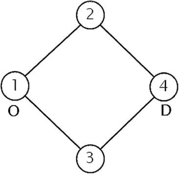
Simple example of network topology for performance and correlation assessment.

Equation 23 may be derived, or bounded for large networks, by a recursive decomposition algorithm, similar to that presented in Liu and Li (2012). Based on Equations 21–23, the network reliability in Figure 1 is favorably affected by a positive correlation between Events F₁ and F₄, and a negative correlation between F₂ and F₃. The first term in the right-hand side decreases and the increase in P(F₁ ∪ F₄) is weighted by P(F₂ ∩ F₃) (which decreases itself); thus inducing an overall reduction in P_f . Accordingly, the worst correlation scenario for the example network happens when negative correlations exist between F₁ and F₄ besides positively correlated F₂ and F₃ events.

These arguments may be expanded to more complicated networks. The network connectivity reliability is favorably affected by negative correlations among nodes on a cut-set (e.g., Nodes 2 and 3 in Figure 1), as well as positive correlations among nodes on a chain (where nodes are in series), which may include the origin and destination nodes. In small networks, where full network decomposition can be carried out to identify all cut-sets and shortest paths in the network, the impact of correlations on the network reliability may be qualitatively assessed by examining correlations among nodes on cut-sets or chains. In actual bridge networks with hundreds or thousands of nodes, a full decomposition may not be practical, but simulations-based methods can still quantify the impact of correlations, as presented in a case study in the companion Application paper. For quantitative assessments, realizations of bridge failures consistent with their correlation values are simulated and used in Monte Carlo simulations. This process is discussed in Stages B.i and B.ii of the BRAN methodology, which is elaborated on in the following section.

Generating Realizations of Correlated Bridge Failures (Stages B.I and B.Ii)

The extra correlations are represented by a correlation matrix among bridge failure probabilities whose entries present the correlation ratios. The bridge failure probabilities and the correlation matrix combine into a probability matrix describing joint bridge failure probabilities, which is in turn used to generate realizations of correlated bridge failures for Monte Carlo simulations to evaluate the network connectivity reliability.

The extra correlations must ideally be estimated from sufficient number of detailed post-earthquake reconnaissance reports that offer correlations among bridge failures based on similarities in factors such as maintenance and retrofit schedule, construction methods, and traffic loads. However, unlike correlations among seismic intensities for probabilistic seismic hazard analysis, extra correlations are often overlooked in the literature of transportation network reliability, and data-driven estimates are not currently available due to a lack of data. Therefore, and without the loss of generality, this study exploits three sources of information to estimate extra correlations in the form of bridge condition ratings, the functional level of roads in the network, and the topological information from the layout of the network. The companion Application paper explains how the three sources represent factors affecting the structural vulnerability of bridges. The rest of this section assumes that an estimated correlation matrix is already formed.

Generating realizations of correlated bridge failures is equivalent to simulating samples from an n-dimensional (n being the number of bridges in the network) binary random variable, as the state of each bridge takes a value of 0 for survival and 1 for failure. The expected value of the n-dimensional binary random variable, therefore, is also the vector of marginal probabilities (bridge failure probabilities from Stage A) while its covariance matrix can be established from a correlation matrix ( R ) informed by extra correlations. Among the different established methods in the literature to simulate samples from binary random variables (e.g., Emrich and Piedmonte 1991, Park et al. 1996, Lunn and Davies 1998), this research adopts an algorithm based on the general dichotomized Gaussian method (DGM). The DGM is preferred over other methods for its general applicability, especially when negative correlations exist.

The DGM procedure forms an associated n-dimensional normal random variable from the binary random variable. The covariance matrix ( S ) of the associated normal random variable is derived from the marginal probabilities and the correlation matrix for the binary random variable ( R ). To generate samples from the original binary random variable, simulated samples from the normal random variable are dichotomized based on their signs. The details of DGM may be found in Emrich and Piedmonte (1991) and Bocchini and Frangopol (2011).

Prior to applying DGM or any method of choice to simulate samples from the multidimensional binary random variable, the correlation matrix R must be compatible with the marginal probabilities. However, the estimated correlation ratios among bridge failure probabilities often do not strictly comply with the requirements originating from bridge failure probabilities themselves. The compatibility conditions arise from basic rules of probabilities and limit the range of admissible values for the correlation ratio between pairs of marginal probabilities. Equations 24 and 25 state the necessary compatibility conditions among probabilities of failure:

\max (0, P_{i} + P_{j} - 1) \leq P_{i j} \leq \min (P_{i}, P_{j}), i \neq j

(24)

P_{i} + P_{j} + P_{k} - P_{i j} - P_{i k} - P_{j k} \leq 1, i \neq j \neq k

(25)

where P_i is bridge i‘s probability of failure, and P_ij is the joint probability of failure between bridges i and j. In order to check for compatibility conditions, the probability matrix P _n×n maybe established from the marginal probabilities and correlation matrix R in which the diagonal entries are the marginal probabilities and off-diagonal entries are the joint probabilities computed from Equation 26:

P_{i j} = P_{i} P_{j} + R_{i j} \sqrt{P_{i} (1 - P_{i}) P_{j} (1 - P_{j})}

(26)

where R_ij is the correlation ratio between the failure probabilities of bridges i and j. Equation 26 is derived from the definition of the correlation ratio between two binary random variables where the expected values are P_i and P_j and the variances are P_i(1 – P_i) and P_j(1 – P_j), respectively.

If the joint probabilities in the probability matrix do not satisfy the necessary compatibility conditions (Equations 24 and 25), they need to be modified accordingly to be within the admissible range, which is a range of values that comply with the compatibility conditions. Equation 26 may then be used to back-calculate the admissible ranges for the correlation ratios when solved for R_ij. The incompatibility of estimated correlation values with the admissible range has been reported in the literature, for example in Bocchini and Frangopol (2011).

The compatibility modification is performed by mapping the elements of the correlation matrix into their respective admissible range. Two auxiliary matrices, R _min and R _max, store the minimum and maximum allowable correlation ratios, respectively, for all the elements of the correlation matrix. The modification involves linearly mapping the correlation ratios R_ij from their original range to [R_min(i, j), R_max(i, j)]. The modified correlation matrix R ₀^′ is constructed by Equation 27 and is ready to be used in simulating samples from the multidimensional binary random variable:

R_{0}^{'} = R_{\min} + \frac{R_{\max} - R_{\min}}{\max (R) - \min (R)} (R - \min (R) \times 1)

(27)

where min( R ) and max( R ) are the scalar overall minimum and maximum correlation ratios in the correlation matrix, respectively, and 1 _n _× _n denotes a matrix of ones. To investigate the sensitivity of network reliability estimates to the correlation values, the elements of the original correlation matrix are shifted toward either min( R ) or max( R ), resulting in more negative or positive correlation levels, respectively. Since Equation 27 represents a linear mapping, any shift toward the boundaries in the original correlation ratio range results in a proportional shift in the modified correlation matrix toward R _min or R _max, as:

R_{λ}^{'} = {\begin{matrix} R_{0}^{'} + λ (R_{\max} - R_{0}^{'}) & λ \in [0, 1] \\ R_{0}^{'} + λ (R_{0}^{'} - R_{\min}) & λ \in [- 1, 0] \end{matrix}

(28)

where R _λ ^′ is the shifted modified correlation matrix and λ is the level of overall deviations from the original correlation estimates.

Although modifying the correlation matrix to satisfy the compatibility conditions is necessary for its applicability, such modifications may result in deviations from the originally estimated correlation values. The difference in correlation matrix 2-norm before and after the compatibility adjustments offers a metric to quantify the level of modifications. Equation 29 introduces the error metric based on matrix 2-norm:

E = \frac{‖ R - R^{'} ‖}{\max (‖ R - R_{\min} ‖, ‖ R - R_{\max} ‖)}

(29)

where E denotes the normalized change in the 2-norm of the correlation matrix, and R ^′ is the modified correlation matrix, either from the original correlation estimates or the shifted values (Equations 27 or 28, respectively).

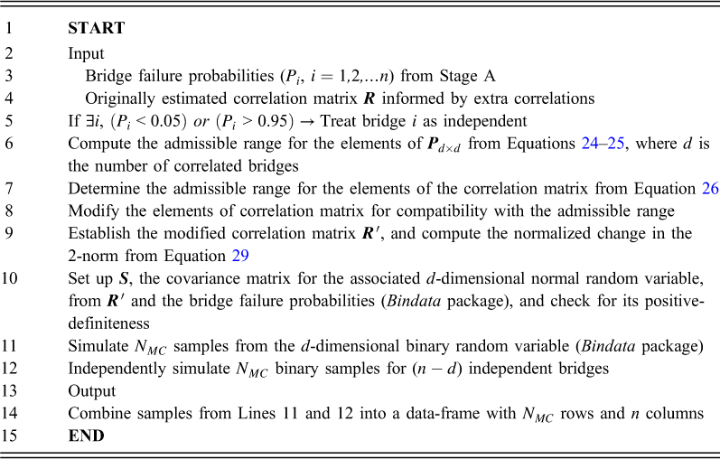
The admissible range for P_ij (and consequently R_ij) can be very tight for extreme probabilities of failure. In particular, the difference between P_ij and P_iP_j becomes negligible in extreme cases and therefore, the binary random variables representing bridges i and j can be treated as independent random variables. Appendix A provides a proof for the rationality of this assumption when the failure probabilities are either very large or very small. Independent treatment of extreme failure probabilities reduces the dimensionality of the binary random variable since the correlated samples only need to be generated for correlated bridge failures. In addition to enhancing the computational efficiency, the reduction of dimensionality prevents numerical errors produced by the narrow admissible ranges in establishing matrix S in DGM. In real bridge networks with large number of bridges, such size reduction may vastly improve the applicability of DGM in terms of the computation time. Finally, matrix S must be checked for positive-definiteness before it can be used in DGM to simulate correlated bridge failures.

Table 3 illustrates the steps to simulate correlated bridge failures. Extreme failure probabilities are considered as values larger than 0.95 or smaller than 0.05. The open source statistical package Bindata (Leisch et al. 1998) written in R (R Development Core Team 2010) is used to simulate samples of correlated binary failures after forming matrix S . The result is N_MC records of realized failures (0 for survival, 1 for failure) for n bridges in the network (a data-frame of N_MC rows and n columns) which are directly applicable for Monte Carlo simulations.

Table 3

Generating realizations of correlated bridge failures for Monte Carlo simulations

1	START
2	Input
3	Bridge failure probabilities (P_i, i = 1,2,...n) from Stage A
4	Originally estimated correlation matrix R informed by extra correlations
5	If ∃i, (P_i < 0.05) or (P_i > 0.95) → Treat bridge i as independent
6	Compute the admissible range for the elements of P _{d x d} from Equations 24-25, where d is the number of correlated bridges
7	Determine the admissible range for the elements of the correlation matrix from Equation 26
8	Modify the elements of correlation matrix for compatibility with the admissible range
9	Establish the modified correlation matrix R ‘, and compute the normalized change in the 2-norm from Equation 29
10	Set up S, the covariance matrix for the associated d-dimensional normal random variable, from R’ and the bridge failure probabilities (Bindata package), and check for its positive-definiteness
11	Simulate N_MC samples from the d-dimensional binary random variable (Bindata package)
12	Independently simulate N_MC binary samples for (n - d) independent bridges
13	Output
14	Combine samples from Lines 11 and 12 into a data-frame with N_MC rows and n columns
15	END

Network-Level Reliability Assessment (Stage B.Iii)

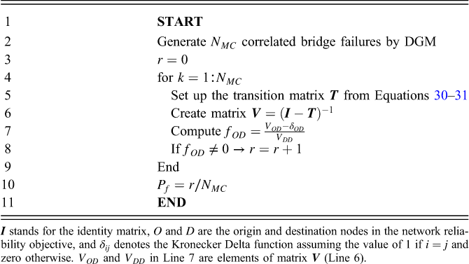
The data-frame of correlated bridge failure samples from Stage B.ii are used to evaluate the network reliability by Monte Carlo simulations. This study evaluates the connectivity reliability of the aging bridge network subjected to seismic loading by the Markov chain Monte Carlo simulation approach (MCMC). The MCMC system reliability method is described in detail in Ross (2007), Ching and Hsu (2007), and Rokneddin et al. (2011), although for independent failures. The bridge network is modeled as a graph where each bridge is a node and the connecting highway segments represent the connecting links. MCMC models the network connectivity reliability by assuming a Markov Chain with transition probability matrix T in which each entry T_ij is the probability that a random walker can move from node i to node j in one step:

T_{i j} = {\begin{array}{l} \frac{1}{k_{i}} \times \max (0, 1 - \frac{w_{j}}{b_{j}}), & n o d e s & i a n d j a r e d i r e c t l y c o n n n e c t e d \\ 0, & i = j, & i a n d j n o t d i r e c t l y c o n n n e c t e d, & o r k_{i} = 0 \end{array}

(30)

where k_i is the out-degree of node i, b_j denotes the reliability (one minus probability of failure) of node j, and w_j is a simulated sample from a uniform distribution in [0, 1]. For each Monte Carlo simulation, connectivity is retained if the random walker has non-zero probability to reach the destination from the origin. The network connectivity reliability is then computed by dividing the number of simulations in which the network remains connected over the total number of simulations.

The original MCMC algorithm requires modification in order to accommodate correlated binary samples simulated by the DGM. The modified algorithm is summarized in Table 4. In particular, simulating w_j in Equation 30 is modified to comply with the correlated failures (note that b_j is directly derived from Stage A and is not impacted by extra correlations):

w_{j} = {\begin{matrix} u_{j} \in [b_{j}, 1], & bridge j fails \\ u_{j} \in [0, b_{j}], & bridge j survives \end{matrix}

(31)

where u_j is a uniform random variable. This modification ensures T_ij = 0 if bridge j fails according to the correlated binary samples generated by DGM and makes the simulations compatible with the derived data-frame of correlated bridge failures from Stage B.ii.

Table 4

Algorithm for MCMC network reliability method with correlated bridge failures

1	START
2	Generate N_MC correlated bridge failures by DGM
3	r = 0
4	for k = 1: N_MC
5	Set up the transition matrix T from Equations 30-31
6	Create matrix $V = {(1 - T)}^{- 1}$
7	Compute $F_{O D} = \frac{V_{O D} - δ_{O D}}{V_{D D}}$
8	If $f_{O D} \neq 0 \to r = r + 1$
9	End
10	$P_{f} = r / N_{M C}$
11	END

I stands for the identity matrix, O and D are the origin and destination nodes in the network reliability objective, and δ_ij denotes the Kronecker Delta function assuming the value of 1 if i = j and zero otherwise. V_OD and V_DD in Line 7 are elements of matrix V (Line 6).

Network connectivity reliability, as described in this section, applies to bridges with binary states (failure and survival), and therefore, bridges in extensive damage state and beyond are considered out of service, as described in Stage A.iii. However, multi-state bridges (partially functional) can be considered with other types of network reliability analysis, for example, if the network limit state is defined based on the overall travel time throughout the network instead of connectivity between (O-D) pairs. Examples of network reliability analysis with multi-state bridges exist in the literature (e.g., Lee and Kiremidjian 2007).

The network probability of failure (P_f in Table 4) represents the outcome of applying the BRAN methodology and help stakeholders of the transportation system to assess risks to the functionality of the network in the event of a strong ground motion. The network reliability method with correlated failures also enables ranking the criticality of bridges for preventive measures and disaster relief (Rokneddin et al., 2011). Assessing such criticalities enables owners to make more informed decisions when allocating funds for necessary maintenance and seismic retrofitting actions.

Conclusions

This paper proposes a two-stage bridge reliability assessment in networks (BRAN) methodology to allow the incorporation of data available from field instrumentation of bridges and different sources affecting simultaneous bridge failures in assessing the seismic reliability of aging bridge networks. In Stage A, the seismic fragilities of aging bridges within a bridge network are evaluated using parameterized fragility models and field instrumentation data. Since it is impractical to instrument every bridge in the network, Kriging, a spatial interpolation procedure, is implemented to determine the values of aging parameters at non-instrumented bridge locations from a limited number of instrumented bridges. The updated posterior estimates of the deterioration parameters are obtained by Bayesian updating of historical estimates of deterioration parameters with the interpolated values. The updated values are then used to determine bridge specific failure probabilities through the parameterized fragility models. However, such factors as the structural conditions of bridges, type of the roads they carry, traffic, and topological implications of the bridge network impose extra correlations among the failure probabilities that are often impractical to include in the analytical bridge modeling, particularly on a structure-by-structure basis. Nevertheless, the impact of extra correlations on network reliability estimates may be significant, depending on specific correlation ratio signs and the topology of the network. Therefore, extra correlations are included in Stage B, which estimates the connectivity reliability of the bridge network between critical origin and destination nodes. This paper shows that the favorable or adverse impact of accounting for the extra correlations on network reliability may be identified trend-wise by studying cut-sets and paths from the origin to the destination, even without a simulation-based network reliability assessment. The more realistic network reliability estimates achieved by enhanced fragility evaluations of aging bridges and by considering extra correlations may also influence the prioritization of bridges for maintenance and seismic retrofitting.

To facilitate the inclusion of extra correlations in future studies, a practical approach based on the general dichotomized Gaussian method (DGM) is used in Stage B to simulate correlated bridge failures, which become the input for the modified Markov chain Monte Carlo (MCMC) reliability method to assess network-level performance. Regardless of the approach to evaluate pairwise correlations among bridge failure probabilities, the established correlation matrix needs modifications to comply with the necessary conditions which impose an admissible range for the correlation ratios based on bridge failure probabilities. Accordingly, the elements of the correlation matrix are modified to comply with their respective admissible ranges. Such modifications may result in deviations from the originally estimated correlation values, especially in large networks.

The companion Application paper demonstrates the BRAN methodology applied to an existing large aging transportation network in the state of South Carolina, consisting of structurally different bridge types with varying aging mechanisms. The fragility estimates corresponding to each of these bridges are evaluated for a scenario earthquake, and the construction of the extra correlations matrix from available data sources is discussed. The network reliability is assessed for a range of correlation values—including the values established from the available data sources—to study the impact of extra correlations. The correlated network reliability estimates are also compared to the reliability estimates for the same network without accounting for correlations to highlight the impact of such extra correlations and their relevance in decision support for distributed systems.

Footnotes

Acknowledgements

This research was partially supported by the National Science Foundation under Grant No. CMMI-0923493. Any opinions, findings, and conclusions or recommendations expressed in this material are those of the authors and do not necessarily reflect the views of the National Science Foundation.

Appendix A

Please refer to the Electronic Supplement in the online edition of this paper.

References

American Society of Civil Engineers (ASCE), 2013. ASCE | 2013 Report Card for America's Infrastructure | Bridges: Conditions & Capacity, available at http://www.infrastructurereportcard.org/a/#p/bridges/conditions-and-capacity (last accessed 15 May 2014).

Alipour

, Shafei

, and Shinozuka

, 2011. Performance evaluation of deteriorating highway bridges located in high seismic areas, Journal of Bridge Engineering 16, 597–611.

Baker

J. W.

, and Cornell

C. A.

, 2005. A vector-valued ground motion intensity measure consisting of spectral acceleration and epsilon, Earthquake Engineering & Structural Dynamics 34, 1193–1217.

Bocchini

, and Frangopol

D. M.

, 2011. Generalized bridge network performance analysis with correlation and time-variant reliability, Structural Safety 33, 155–164.

Box

G. E. P.

, and Wilson

K. B.

, 1951. On the experimental attainment of optimum conditions, Journal of the Royal Statistical Society, Ser. B 13, 1–45.

Bucher

C. G.

, and Bourgund

, 1990. A fast and efficient response surface approach for structural reliability problems, Structural Safety 7, 57–66.

Choe

D.-E.

, Gardoni

Paolo

, Rosowsky

, and Haukaas

, 2008. Probabilistic capacity models and seismic fragility estimates for RC columns subject to corrosion, Reliability Engineering & System Safety 93, 383–393.

Choe

D.-E.

, Gardoni

Paolo

, Rosowsky

, and Haukaas

, 2009. Seismic fragility estimates for reinforced concrete bridges subject to corrosion, Structural Safety 31, 275–283.

Congdon

, 2007. Bayesian Statistical Modelling, John Wiley & Sons, New York, 596 pp.

10.

Cressie

N. A. C.

, 1993. Statistics for Spatial Data, John Wiley & Sons, New York, 928 pp.

11.

Emrich

L. J.

, and Piedmonte

M. R.

, 1991. A method for generating high-dimensional multivariate binary variates, The American Statistician 45, 302–304.

12.

Enright

M. P.

, and Frangopol

D. M.

, 1998. Probabilistic analysis of resistance degradation of reinforced concrete bridge beams under corrosion, Engineering Structures 20, 960–971.

13.

Enright

M. P.

, and Frangopol

D. M.

, 1999. Condition prediction of deteriorating concrete bridges using Bayesian updating, Journal of Structural Engineering 125, 1118–1125.

14.

Gassman

S. L.

, and Tawhed

W. F.

, 2004. Nondestructive assessment of damage in concrete bridge decks, Journal of Performance of Constructed Facilities 18, 220–231.

15.

Ghosh

, and Padgett

J. E.

, 2010. Aging considerations in the development of time-dependent seismic fragility curves, Journal of Structural Engineering 136, 1497–1511.

16.

Ghosh

, and Padgett

J. E.

, 2012. Impact of multiple component deterioration and exposure conditions on seismic vulnerability of concrete bridges, Earthquakes and Structures, in press.

17.

Goos

, and Jones

, 2011. Optimal Design of Experiments: A Case Study Approach, John Wiley & Sons, New York, 304 pp.

18.

Guan

X. L.

, and Melchers

R. E.

, 2001. Effect of response surface parameter variation on structural reliability estimates, Structural Safety 23, 429–444.

19.

Huang

, Gardoni

Paolo

, and Hurlebaus

, 2009. Probabilistic capacity models and fragility estimates for reinforced concrete columns incorporating NDT data, Journal of Engineering Mechanics 135, 1384–1392.

20.

Jayaram

, and Baker

J. W.

, 2009. Correlation model for spatially distributed ground-motion intensities, Earthquake Engineering & Structural Dynamics 38, 1687–1708.

21.

Jayaram

, and Baker

J. W.

, 2010. Efficient sampling and data reduction techniques for probabilistic seismic lifeline risk assessment, Earthquake Engineering & Structural Dynamics 39, 1109–1131.

22.

Kang

W.-H.

, Song

, and Gardoni

, 2008. Matrix-based system reliability method and applications to bridge networks, Reliability Engineering and System Safety 93, 1584–1593.

23.

Kazmer

D. O.

, 2009. Plastics Manufacturing Systems Engineering, Hanser Publishers, Cincinnati, OH, 502 pp.

24.

Kiefer

, and Wolfowitz

, 1959. Optimum designs in regression problems, The Annals of Mathematical Statistics 30, 271–294.

25.

Kiremidjian

, Stergiou

, and Lee

, 2007. Issues in seismic risk assessment of transportation networks, Earthquake Geotechnical Engineering 6, 461–480.

26.

Koutsourelakis

P. S.

, 2010. Assessing structural vulnerability against earthquakes using multidimensional fragility surfaces: A Bayesian framework, Probabilistic Engineering Mechanics 25, 49–60.

27.

Krige

D. G.

, 1951. A Statistical Approach to Some Mine Valuation and Allied Problems on the Witwatersrand, University of the Witwatersrand, 272 pp.

28.

Lee

, and Kiremidjian

A. S.

, 2007. Uncertainty and correlation for loss assessment of spatially distributed systems, Earthquake Spectra 23, 753–770.

29.

Leisch

, Weingessel

, and Hornik

, 1998. On the generation of correlated artificial binary data, Working Paper No. 13, Vienna University of Economics and Business Administration, Vienna, Austria.

30.

Liu

, and Li

, 2012. An improved cut-based recursive decomposition algorithm for reliability analysis of networks, Earthquake Engineering and Engineering Vibration 11, 1–10.

31.

Lunn

A. D.

, and Davies

S. J.

, 1998. A note on generating correlated binary variables, Biometrika 85, 487–490.

32.

Mackaness

, and Beard

, 1993. Visualization of interpolation accuracy, in Proceedings, Auto Carto, 228–237.

33.

Marsh

P. S.

, and Frangopol

D. M.

, 2008. Reinforced concrete bridge deck reliability model incorporating temporal and spatial variations of probabilistic corrosion rate sensor data, Reliability Engineering & System Safety 93, 394–409.

34.

Mazzoni

, McKenna

, Scott

M. H.

, and Fenves

G. L.

, 2009. OpenSees Command Language Manual, Command Language Manual, University of California, Berkeley.

35.

Moncmanová

, 2007. Environmental Deterioration of Materials, WIT Press, Southampton, UK.

36.

Mount

, Aplin

, and Priestnall

, 2008. Representing, Modeling, and Visualizing the Natural Environment, CRC Press, Boca Raton, FL, 416 pp.

37.

Myers

J. C.

, 1997. Geostatistical Error Management: Quantifying Uncertainty for Environmental Sampling and Mapping, John Wiley & Sons, New York, 571 pp.

38.

Nielson

B. G.

, 2005. Analytical Fragility Curves for Highway Bridges in Moderate Seismic Zones, Ph.D. Thesis, Georgia Institute of Technology, Atlanta, GA.

39.

Nielson

B. G.

, and DesRoches

, 2007. Analytical Seismic Fragility Curves for Typical Bridges in the Central and Southeastern United States, Earthquake Spectra 23, 615–633.

40.

Olea

R. A.

, 1999. Geostatistics for Engineers and Earth Scientists, Springer, New York, 303 pp.

41.

Padgett

J. E.

, and DesRoches

, 2007. Bridge Functionality Relationships for Improved Seismic Risk Assessment of Transportation Networks, Earthquake Spectra 23, 115–130.

42.

Park

C. G.

, Park

, and Shin

D. W.

, 1996. A simple method for generating correlated binary variates, The American Statistician 50, 306–310.

43.

R Development Core Team, 2010. The R Project for Statistical Computing, available at http://www.r-project.org/ (last accessed 30 December 2011).

44.

Rajashekhar

M. R.

, and Ellingwood

B. R.

, 1993. A new look at the response surface approach for reliability analysis, Structural Safety 12, 205–220.

45.

Reimann

, 2008. Statistical Data Analysis Explained: Applied Environmental Statistics with R, John Wiley & Sons, New York, 362 pp.

46.

Rix

G. J.

, and Fernandez

J. A.

, 2004. Earthquake Ground Motion Simulation, available at http://www.ce.gatech.edu/research/mae_ground_motion/ (last accessed 19 October 2009).

47.

Rokneddin

, Ghosh

Jayadipta

, Dueñas-Osorio

, and Padgett

, 2011. Bridge retrofit prioritization for aging transportation networks subject to seismic hazards, Structure and Infrastructure Engineering, in press.

48.

Simpson

T. W.

, Poplinski

J. D.

, Koch

P. N.

, and Allen

J. K.

, 2001. Metamodels for computer-based engineering design: Survey and recommendations, Engineering With Computers 17, 129–150.

49.

Stewart

M. G.

, 2004. Spatial variability of pitting corrosion and its influence on structural fragility and reliability of RC beams in flexure, Structural Safety 26, 453–470.

50.

Stewart

M. G.

, and Suo

, 2009. Extent of spatially variable corrosion damage as an indicator of strength and time-dependent reliability of RC beams, Engineering Structures 31, 198–207.

51.

Straub

, and Armen Der Kiureghian

, 2010. Bayesian network enhanced with structural reliability methods: Methodology, Journal of Engineering Mechanics 136, 1248–1258.

52.

Strauss

, Frangopol

D. M.

, and Kim

, 2008. Use of monitoring extreme data for the performance prediction of structures: Bayesian updating, Engineering Structures 30, 3654–3666.

53.

The MathWorks, 2004. MATLAB, The MathWorks, Inc., Natick, MA.

54.

Towashiraporn

, 2004. Building Seismic Fragilities Using Response Surface Metamodels, Ph.D. Thesis, Georgia Institute of Technology, Atlanta, GA.

55.

Trauth

M. H.

, Gebbers

R. (CON)

, and Marwan

N. (CON)

, 2010. MATLAB® Recipes for Earth Sciences, Springer, New York.

56.

Wen

Y. K.

, and Wu

C. L.

, 2001. Uniform hazard ground motions for Mid-America cities, Earthquake Spectra 17, 359–384.

57.

Wesson

R. L.

, Perkins

D. M.

, Luco

, and Karaca

, 2009. Direct calculation of the probability distribution for earthquake losses to a portfolio, Earthquake Spectra 25, 687–706.

58.

Wesson

R. L.

, and Perkins

D. M.

, 2001. Spatial correlation of probabilistic earthquake ground motion and loss, Bulletin of the Seismological Society of America 91, 1498–1515.

Supplementary Material

Please find the following supplemental material available below.

For Open Access articles published under a Creative Commons License, all supplemental material carries the same license as the article it is associated with.

For non-Open Access articles published, all supplemental material carries a non-exclusive license, and permission requests for re-use of supplemental material or any part of supplemental material shall be sent directly to the copyright owner as specified in the copyright notice associated with the article.

0.00 MB

0.03 MB