A Framework for Post-Earthquake Response Planning in Emerging Seismic Regions: An Oklahoma Case Study

Abstract

This paper presents a framework for establishing post-earthquake response protocols in regions facing emerging seismic hazards through a case study of Oklahoma bridges. First, it establishes the need for new attenuation models for the Oklahoma area because of the poor fit of current attenuation models. Then, two methods are established to inspect bridges after an earthquake: smart inspection radii and ShakeCast. The smart radii use a modified version of the Campbell (2003) attenuation model to determine seismic demand and a trigger S₁ value to represent bridge capacity. This trigger S₁ value is validated by calculating slight HAZUS fragility curves for past earthquakes. ShakeCast is an online resource from USGS that uses real-time ground motion data (i.e., a ShakeMap) as seismic demand and modified HAZUS fragility curves to represent bridge capacity. Because of better-informed data on the ground shaking levels, ShakeCast recommends significantly fewer inspections than inspection radii, translating to cost savings for the Oklahoma Department of Transportation.

Introduction

The seismicity of places such as California and the New Madrid seismic zone is well established. However, new areas are emerging, such as Oklahoma, Kansas, and Texas, that are experiencing induced seismicity (Petersen et al. 2017). Induced seismicity effects are not only limited to the United States, but also other countries, including Canada, China, and the United Kingdom (McGarr et al. 2015). The induced seismicity is not as well documented as naturally occurring seismicity. This study focuses on Oklahoma, but the framework proposed here is applicable to other emerging seismic regions.

Seismicity in Oklahoma

Since 2009, there has been a dramatic increase in the number of earthquakes in Oklahoma. Oklahoma and the surrounding region have not historically experienced earthquakes at the rate currently observed (McGarr et al. 2015; Figure 1). Studies, such as that by Keranen et al. (2013), have linked the increased rate of seismic activity since 2009 to waste-water injection in disposal wells. The only identified source of natural (tectonic) earthquakes in this region is the Meer's fault in southwest Oklahoma, as reflected in the U.S. Geological Survey (USGS) national seismic hazard maps (Petersen et al. 2014) and, accordingly, the mapped design ground motion data provided by the 2009 AASHTO Guide Specifications for LRFD Seismic Bridge Design (AASHTO 2009). In 2016, the USGS made an effort to incorporate non-tectonic earthquakes (or “induced seismicity”) into the national seismic hazard model (Petersen et al. 2016), but these are not reflected in seismic design provisions. Therefore, concern has arisen about how Oklahoma's infrastructure will handle the increased seismic demand. In particular, the Oklahoma Department of Transportation (ODOT) is concerned about bridge response to earthquakes and the potential for damage.

Figure 1.

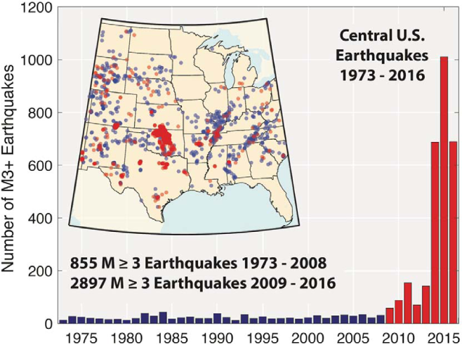
Annual Central U.S. earthquakes 1973–2016 (USGS 2017).

At 12:02:44 Coordinated Universal Time (UTC) on 3 September 2016, a magnitude (M) 5.8 earthquake struck 15 km northwest of Pawnee, Oklahoma. The event was triggered by strike-slip faulting within the interior of the North America plate (USGS 2016d), at a focal depth of 5.6 km and is the largest recorded event in Oklahoma to date. Over the decade prior to this event, Oklahoma experienced nearly 80 other M4.0 or larger events, including two larger than M5.0: the 6 November 2011 M5.7 earthquake near Prague, Oklahoma (USGS 2016c) and the 13 February 2016 M5.1 earthquake near Fairview, Oklahoma (USGS 2016b). A fourth large event (M5.0) occurred on 7 November 2016 near Cushing, Oklahoma (USGS 2016a). These M5.0 and larger events were felt in the surrounding states, caused damage to residential structures, and resulted in minor injuries. The extent of damage to highway bridges has been limited to minor spalling of concrete at one bridge (GEER 2016) and the need to reset a roller bearing on another bridge (W. L. Peters, pers. comm., 20 October 2016) following the M5.8 Pawnee event.

History of Odot'S Post-Earthquake Inspection Protocol

When the earthquake activity began to increase, ODOT had to determine when and how to inspect their bridges after an earthquake. Their initial response was to inspect after every earthquake with a magnitude greater than 3.0. However, as time went on, they found this to be overly conservative.

On 23 January 2015, ODOT revised the protocol to dictate that bridges must be inspected within a 5-mile radius for earthquakes with magnitudes from 4.0 to 4.9, within a 25-mile radius for earthquakes with magnitudes from 5.0 to 5.5, and within a 50-mile radius for earthquakes with magnitudes greater than 5.5. If damage was found within those radii, the inspection radius was expanded by 5 miles (W. L. Peters, pers. comm., February 2017).

This inspection protocol resulted in over 30 inspections in 2015, yet no earthquake-related damage to the bridges was found. ODOT felt that even this was too much and wanted to establish an evidence-based, rigorous procedure. In 2015, they hired a team of consultants led by Infrastructure Engineers, Inc. to revise their post-earthquake bridge inspection protocol. This contract consisted of two phases: Phase I, which would establish an interim post-earthquake bridge inspection protocol, and Phase II, which would develop and implement ShakeCast for Oklahoma. On 1 April 2016, the interim protocol was implemented. Shake-Cast became operational in August 2017.

Evaluation of Current Attenuation Models

The 2008 USGS seismic hazard map groups Oklahoma with the New Madrid seismic zone (Petersen et al. 2008). This zone uses a weighted attenuation model that is a combination of seven different attenuation models. The weights are based on the different types of models (Petersen et al. 2008). Frankel et al. (1996) and Toro et al. (1997) are single-corner finite fault models with weight = 0.1 and 0.2, respectively; Silva et al. (2002) is a single-corner point-source model with weight = 0.1; Atkinson and Boore (2006) is a dynamic-corner frequency source model with weight = 0.1 for both 140 and 200 bar stress drops; Campbell (2003) and Tavakoli and Pezeshk (2005) are hybrid models, each with weight = 0.1; and Somerville et al. (2001) is an extended-source model with weight = 0.2.

Acceleration time histories from seismic stations were acquired for 80 earthquakes that had a magnitude of at least 4.0 occurring between 27 February 2010 and 21 March 2017, using Standing Order for Data (SOD; Owens et al. 2004). Both velocity and acceleration sensor data were collected, but if a station had both sets of data, only the acceleration sensors were used so the station would not be double counted. Stations with only one direction of data recorded were not included. Additionally, each acceleration time history was screened for obvious problems, such as clipping, missing data, noise spikes, etc., which were removed from this study, resulting in a total of 1,286 bidirectional ground motions. These bidirectional ground motions records were processed using standard PEER procedure and used to calculate the spectral response accelerations for each ground motion. In particular, the spectral accelerations reported are the geometric mean of the two horizontal components. Of interest to this work are the 1-s and 0.3-s spectral accelerations (S₁ and S_0.3, respectively).

The calculated S₁ for each station were compiled and compared with predictions made with the attenuation models. Figure 2 compares the station data with the eight attenuation models and the weighted model from the 2008 USGS Seismic Hazard Map for all magnitude 4.0, 4.2, 5.7, and 5.8 Oklahoma earthquakes. For the weighted model, the Frankel et al. (1996) tables do not calculate values for S₁ at epicentral distances less than 9 km or for magnitudes less than 4.4. Therefore, the weighted model was adjusted to not include Frankel for these situations (the weights were divided by 0.9 to redistribute the 0.1 originally for Frankel et al. 1996). Epicentral distance was used instead of hypocentral distance because epicentral distance is used by a majority of the attenuation models. For the models that use hypocentral distances, a depth of 5 km was assumed. Figure 2 shows that most of the attenuation models tend to over predict Oklahoma ground motions, especially at moderate to long distances (20–120 km). Some responses at close distances (<20 km), which contribute the most to the seismic hazard, exceed the predicted values, indicating faster attenuation (Atkinson 2015). Similar trends have been shown for other Central and Eastern U.S. attenuation models (Gupta et al. 2017), such as the model (Shahjouei and Pezeshk 2016) developed as part of the the NGA-East research project (Goulet et al. 2015).

Figure 2.

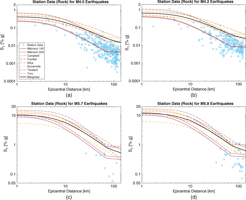
Station data compared with the eight attenuation models and the weighted model from the 2008 USGS Seismic Hazard Map: (a) 360 M4.0 earthquakes, (b) 258 M4.2 earthquakes, (c) the 11 November 2011 M5.7 Prague earthquake, and (d) the 3 September 2016 M5.8 Pawnee earthquake.

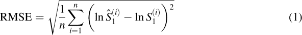
Table 1 shows the root-mean-square error (RMSE) in comparing the station data to each model, namely (Zwillinger 1995):

RMSE = \sqrt{\frac{1}{n} \sum_{i = 1}^{n} {(\ln {\hat{S}}_{1}^{(i)} - \ln S_{1}^{(i)})}^{2}}

(1)

where n is the number of measurements, and

{\hat{S}}_{_{1}}^{(i)}

and

S_{_{1}}^{(i)}

are the ith predicted and measured 1-s spectral accelerations, respectively.

Table 1

The root-mean-square error (RMSE) in comparing the station data to each model and the weighted model for M4.0-M5.8 earthquakes and the RMSE in the model compared to all earthquakes (total). Bold and italics indicate the lowest and highest RMSE, respectively, for a given magnitude

Mag.	Atkinson 140	Atkinson 200	Campbell	Frankel	Silva	Somerville	Tavakoli	Toro	Weighted	n ^*
4.0	0.793	0.806	2.036	n/a	1.303	1.730	1.672	2.357	1.770	360
4.1	0.898	0.899	1.874	n/a	1.253	1.557	1.598	2.166	1.626	227
4.2	0.751	0.750	1.746	n/a	1.140	1.409	1.479	2.052	1.497	258
4.3	0.698	0.695	1.616	n/a	1.012	1.231	1.414	1.874	1.354	110
4.4	1.005	0.993	1.636	1.266	1.166	1.302	1.473	1.880	1.424	151(145)
4.5	0.738	0.730	1.474	0.981	0.924	1.022	1.346	1.718	1.124	16(15)
4.7	0.336	0.299	1.219	0.905	0.785	0.802	1.079	1.541	0.983	50(50)
4.8	0.804	0.778	1.302	1.108	0.899	0.922	1.211	1.551	1.096	23(23)
4.9	0.952	0.902	1.091	0.915	0.903	0.807	1.152	1.238	0.940	11(11)
5.0	0.664	0.680	1.292	1.150	0.912	0.796	1.323	1.466	1.074	23(19)
5.1	0.490	0.621	1.603	1.533	1.034	0.981	1.567	1.775	1.330	17(17)
5.7	0.893	1.036	1.672	1.757	1.438	1.189	1.730	1.882	1.521	10(10)
5.8	0.767	0.906	1.481	1.575	1.173	0.951	1.555	1.612	1.304	30(30)
Total	0.808	0.814	1.787	1.245	1.180	1.452	1.532	2.073	1.542	1286(1275)

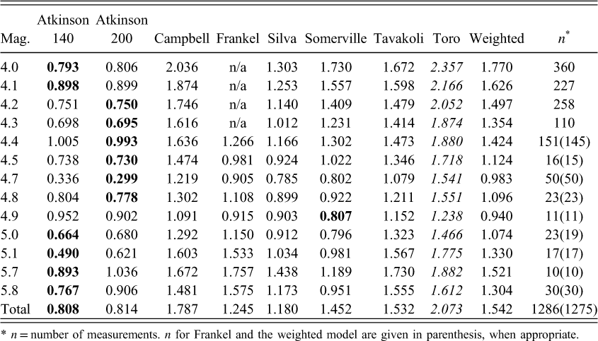
n = number of measurements. n for Frankel and the weighted model are given in parenthesis, when appropriate.

Because of the previously mentioned limitations of Frankel et al. (1996), it cannot be compared to all of the station data, so the incomparable points were omitted when computing RMSE. The RMSE values as well as the figures show that, of the attenuation models considered, Atkinson and Boore (2006) with 140 and 200 bar stress drops best predict ground motions for Oklahoma earthquakes, while Campbell (2003) and Toro et al. (1997) do the worst.

These results show that current attenuation models applied to Oklahoma ground motions display a large degree of variability with differing degrees of accuracy in predicting spectral accelerations needed to establish Oklahoma's response protocol. In the development of an earthquake response protocol, having accurate representation of the ground-motion attenuation is vital. The following section looks at modifying an existing attenuation model in the process of developing an interim protocol for ODOT. In addition, an accurate representation of the vulnerability (fragility) of Oklahoma bridges is sought to enhance the protocol.

Developing Interim Protocol

To revise ODOT's inspection radii, both the capacity of and demand on Oklahoma bridges were considered. Bridge capacity was modeled with fragility functions. The seismic demand was quantified by ground-motion intensity, which was predicted using a ground-motion attenuation model adjusted for soil amplification and calibrated with measured acceleration records from seismic stations in Oklahoma.

Determining Trigger S₁ Value

In order to determine inspection radii, a trigger S₁ value, below which damage is unlikely to be found, must first be established. The probability that a bridge reaches or exceeds the slight (lowest) damage state (DS) for a given S₁ is given by the fragility function

F_{slight} (S_{1}) \equiv P [D S \geq slight | S_{1}] = Φ [\frac{1}{β} \ln (\frac{S_{1}}{{\tilde{S}}_{1}})]

(2)

where Φ[·] is the standard normal cumulative distribution function, β is the logarithmic standard deviation, and S~₁ is the median S₁. Based on the HAZUS fragility function (FEMA 2003), β is taken to be 0.6 hereinafter. Determination of S~₁ involves modifying tabulated median S₁ values, denoted S~₁. For some bridge classes, S~₁ is simply taken as the tabulated S~₁, whereas other bridge classes require modification of the tabulated S~₁ by the factor K_shape (i.e., S~₁ = K_shapeS~₁). However, K_shape cannot be calculated a priori because it requires actual (measured) ground motion data:

K_{s h a p e} = \min [2.5 S_{1} / s_{0.3}, 1]

(3)

The 2.5 in Equation 3 is the ratio between S_0.3 and S₁ for the standard code-based spectral shape for which the HAZUS fragility functions were derived (Basöz and Mander 1999).

Because the slight HAZUS fragility function cannot be calculated a priori for all bridge classes, Caltrans uses a trigger S₁ value of 0.10 g instead of a fragility function for slight damage. This value comes from their experience of not seeing damage on bridges that experience an S₁ less than 0.10 g (L. Turner, pers. comm., 2015). ODOT, however, has not had Caltrans’ experience to determine if an S₁ of 0.10 g is also valid in Oklahoma. Therefore, the tabulated S~₁ values for the slight damage state in HAZUS were examined and compared for California (CA) and non-California (non-CA) bridges. There were four instances where the same bridge had a different value for a CA bridge versus a non-CA bridge. All four cases were conventionally designed, simply supported bridges with multi-column bents, which were distinguished by the main span material and length: concrete (HWB5/HWB6), pre-stressed concrete (HWB17/HWB18), and steel (length ≥20 m, HWB12/HWB13; length <20 m, HWB24/HWB25). Each of these instances gave the CA bridges and the non-CA bridges an S~₁ of 0.30 and 0.25 g, respectively (FEMA 2003). Using this information, the ratio between the two bridges (0.25 ÷ 0.30) was applied to the S₁ value of 0.10 g from Caltrans to give an S₁ value of 0.0833 g for Oklahoma. Note that here “conventionally designed” refers to non-CA bridges built before 1990 or CA bridges built before 1975. Bridges built after these dates are designated “seismically designed” because they were designed in accordance with the AASHTO seismic provisions or satisfactory seismic provisions, respectively (Basöz and Mander 1999).

To ensure a greater level of confidence, the value of 0.0833 g for Oklahoma was treated as the median S₁ for a base fragility function (Figure 3). Trigger S₁ values for a chosen probability P of slight damage are determined from the following equation:

S_{1}^{trigger} (P) = {\tilde{S}}_{1} \exp (β Φ^{- 1} [P])

(4)

where S~₁ = 0.0833 g and β = 0.6. The trigger S₁ values for 10%, 25%, 33%, and 50% probability of being in the slight damage state were found to be 0.0386, 0.0556, 0.0643, and 0.0833 g, respectively. ODOT chose 25% probability of being in the slight damage state as the value they felt most comfortable with, so 0.0556 g was chosen as the trigger value.

Figure 3.

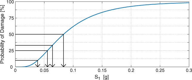
Base fragility curve used for Oklahoma bridges. Note β = 0.6.

Trigger Value Validation: Computing Slight Fragility Curve

Ground motion data (S₁, S_0.3) from past earthquakes can be extracted from seismic stations and ShakeMap to determine whether or not the proposed trigger value is conservative.

Validation Using Seismic Station Data

Using the same set of data as used in Evaluation of Current Attenuation Models, the S₁/S_0.3 ratio was computed for each station from each earthquake. These values were then plotted against station distance from epicenter (Figure 4a) and earthquake magnitude (Figure 4b). No correlation is observed between magnitude or distance and S₁/S_0.3 ratio. Therefore, K_shape can be assumed to be independent of magnitude and distance for Oklahoma.

Figure 4.

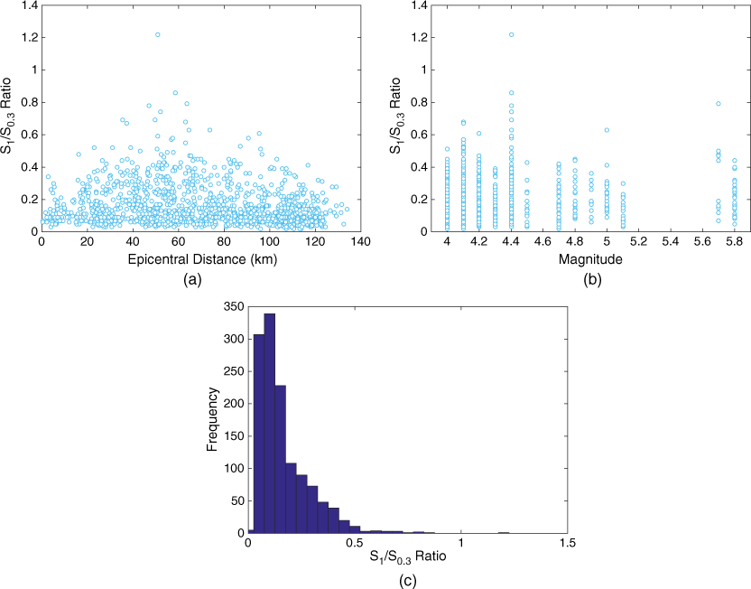
S₁/S_0.3 ratios computed at each station plotted against (a) epicentral distance, (b) earthquake magnitude, and (c) frequency of occurrence.

Figure 4c shows a histogram of all the recorded ratios. The mean and median of this data is 0.16 and 0.12, respectively. The fact that most of the S₁/S_0.3 ratios are less than 0.4 (= 1 ÷ 2.5) indicates that Oklahoma earthquakes tend to have higher frequency content than the code-based spectral shape used to derive the HAZUS fragility functions. This, in turn, means K_shape is less than unity (Equation 3), resulting in reduced slight fragility curve medians (i.e., more vulnerable than the “standard bridge”).

The variability in the ratio S₁/S_0.3 translates to uncertainty in the median S₁ through K_shape (Equation 3). The uncertainty in S~₁ can be accounted for in the estimate of the probability of observing slight damage, for a given ground motion intensity S₁, by marginalizing over the distribution of S~₁, denoted f (S~₁):

P [DS \geq slight | S_{1}] = \int_{0}^{\infty} P [DS \geq slight | S_{1}, {\tilde{S}}_{1}] f ({\tilde{S}}_{1}) d {\tilde{S}}_{1}

(5)

where P[DS ≥ slight | S₁, S~₁] is the slight fragility curve given by Equation 2 with uncertain S~₁. This integral can be calculated using Monte Carlo integration (Robert and Casella 2004). Equation 5 is approximated by the empirical average,

P [D S \geq slight | S_{1}] \approx \frac{1}{N} \sum_{j = 1}^{N} P [D S \geq slight | S_{1}, {\tilde{S}}_{1}^{(j)}]

(6)

where

{\tilde{S}}_{1}^{(j)} (j = 1, \dots, N)

(j = 1,…, N) are independent and identically distributed (i.i.d.) samples generated from the density f, taken to be

{\tilde{S}}_{1}^{(j)} = K_{s h a p e}^{(j)} {\tilde{s}}_{1}

where the

K_{s h a p e}^{(j)}

are determined from the measured S₁/S_0.3 values (Figure 4c). The tabulated S~₁ is based on the bridge class being considered.

According to the HAZUS manual (FEMA 2003), the lowest tabulated (unmodified) median S₁ for slight damage for non-CA bridges that include K_shape is 0.60 g, which was for concrete (HWB10) and prestressed concrete (HWB22) conventionally designed, continuous bridges. Evaluating Equation 6 at the trigger S₁ value of 0.0556 g assuming this tabulated median S₁ (0.6 g), the probability is determined to be 9%, which is below the 25% used in establishing the trigger value. This indicates that the base fragility curve is conservative relative to the HAZUS slight fragility curve for these bridge classes.

For bridges that do not require modification by K_shape, S~₁ is a non-random variable (i.e., deterministic) and Equation 2 can be applied directly. For these bridges, the lowest tabulated median S₁ for slight damage is 0.25 g for concrete (HWB5), prestressed concrete (HWB17), and steel (length ≥20 m, HWB12; length <20 m, HWB24) conventionally designed (non-CA), simply supported bridges with multi-column bents. This corresponds to a 0.6% probability of slight damage at the trigger S₁ value of 0.0556 g, which would indicate that bridges with K_shape are more at risk than those without. However, the bridges damaged during the M5.8 Pawnee earthquake were both HWB12, which do not require K_shape modification.

Validation Using ShakeMap Grid Data

Due to a relatively sparse seismograph network in Oklahoma, station data tends to be far from the earthquake epicenter (>10 km), corresponding to measured shaking levels that produce low probabilities of damage. Therefore, ShakeMap grid S₁ and S_0.3 values (USGS 2015b) were also used to calculate probabilities of slight damage assuming the lowest tabulated median value for bridges with K_shape modification (i.e., S~₁ = 0.6 g) and without K_shape modification (i.e., S~₁ = S~₁ = 0.25 g). Contours of probability of slight damage for these two bridge classes are shown in Figures 5 and 6 for the 3 September 2016 M5.8 Pawnee earthquake and the 6 November 2011 M5.7 Prague earthquake, respectively. Note that the Sha-keMaps for these earthquakes (event IDs us10006jxs-9 and 20111106035310-1) utilized the attenuation models Atkinson and Boore (2006) and Campbell (2003), respectively, with magnitude biases fit according to Worden et al. (2010).

Figure 5.

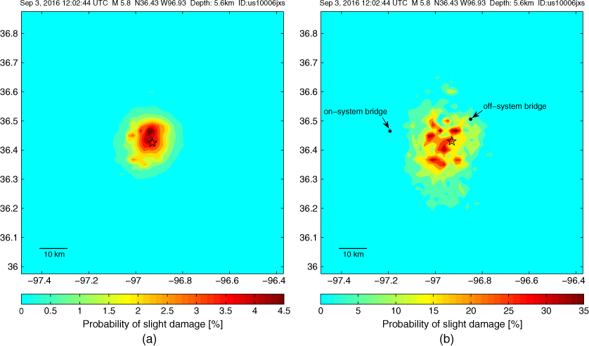
Contours of probability of slight damage for the 3 September 2016 M5.8 Pawnee earthquake based on the HAZUS fragility functions with a median S₁ of (a) 0.6 g modified by K_shape and (b) 0.25 g. The dots indicate the two bridges that experienced slight damage.

Figure 6.

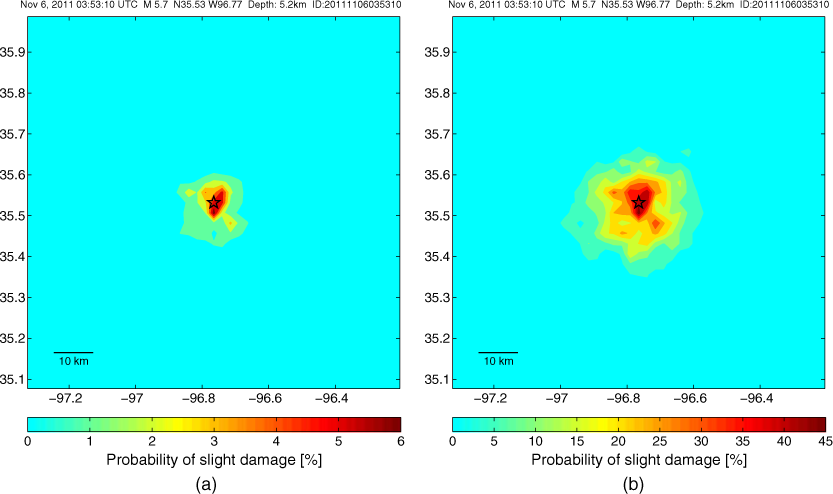
Contours of probability of slight damage for the 6 November 2011 M5.7 Prague earthquake based on the HAZUS fragility functions with a median S₁ of (a) 0.6 g modified by K_shape and (b) 0.25 g

For the M5.8 Pawnee earthquake, the highest probabilities of damage were 4.8% (Figure 5a) and 37.5% (Figure 5b) for bridge classes with and without K_shape modification, respectively. For the M5.7 Prague earthquake, the highest probabilities of damage were 6.4% (Figure 6a) and 47.6% (Figure 6b) for bridge classes with and without K_shape modification, respectively. For both earthquakes, the probability of damage is significantly higher for the bridge classes that do not include K_shape modification. This is due to the relatively high S₁/S_0.3 ratios according to ShakeMap. The average S₁/S_0.3 ratio for the M5.8 Pawnee and M5.7 Prague earthquakes are 0.39 and 0.85, respectively, which are significantly higher than the seismic station data (Figure 4). This results in (modified) median S₁ values of 0.58 and 0.60 g, which are considerably higher than the median S₁ for bridges without K_shape modification (0.25 g).

As previously noted, the two bridges that were damaged during the M5.8 Pawnee earthquake were both HWB12, which do not require K_shape modification. The locations of these bridges are indicated in Figure 5b. The “on-system” bridge (on-system bridges are those on state-owned routes and highway systems, not including locally-owned bridges) was located 24 km from the epicenter and had a roller bearing that came dislodged (W. L. Peters, pers. comm., 2016); the ShakeMap determined S₁ at the bridge site was 0.074 g, which corresponds to a 2% probability of slight damage based on the HAZUS fragility functions. The “off-system” bridge was located 11 km from the epicenter and had spalling of cover concrete at the abutments (GEER 2016); the ShakeMap determined S₁ at the bridge site was 0.103 g, which corresponds to a 7% probability of slight damage. While these probabilities of damage are low, it is worth noting that both bridges experienced shaking in excess of the trigger value (0.0556 g), which would have triggered an inspection. Given that damage was observed at such low expected probabilities of damage, the HAZUS fragility functions may be nonconservative for Oklahoma bridges. However, note that there was one on-system HWB12 bridge that was 15.45 km from the epicenter and experienced a ShakeMap determined S₁ of 0.128 g, but did not receive damage. Also, there were five on-system HWB17 bridges and two on-system HWB5 bridges that experienced S₁ in excess of 0.075 g, but were not damaged. Finally, it is worth noting that the two bridges that were damaged are quite old (built in 1952 and 1927, respectively).

Application to other Emerging Seismic Regions

In the Determining Trigger S₁ Value section, a procedure was described to determine the trigger value for the inspection radii, which was validated based on seismic station data and ShakeMap grid data. An alternative approach that other Departments of Transportation (DOTs) may use is presented here, which adjusts for local ground-motion characteristics (namely, S₁/S_0.3 ratios) to find probabilities of damage based on HAZUS fragility functions. The DOT would choose a probability P of damage that they are comfortable with (e.g., P = 25%). Then, the trigger value level of shaking that produces this probability of damage can be back-calculated from Equation 4 taking the median S₁ to be

\begin{array}{l} {\tilde{S}}_{1} = \min [0.25 g, {\bar{K}}_{shape} 0.6 g] & (non - CA bridges) \end{array}

(7)

where K _shape is the mean K_shape for the region based on recorded S₁/S_0.3 ratios (e.g., 0.39 for Oklahoma). Following this procedure, the trigger S₁ value for Oklahoma assuming a 25% probability of slight damage would have been 0.156 g. Note that this value exceeds the levels of shaking that produced damage to the two bridges in the M5.8 Pawnee earthquake, so it is not conservative. Additional conservatism can be built in by selecting a lower target probability of damage; e.g., a value of P = 2% would have been required to reach a trigger S₁ of 0.074 g (i.e., the ShakeMap determined S₁ at the on-system bridge damaged during the M5.8 Pawnee earthquake). The degree of conservatism strongly depends on the validity of the HAZUS fragility functions for the local bridge inventory; if the fragility functions are nonconservative, then a very low target probability is needed to give a conservative

S_{1}^{t r i g g e r}

Modifying Campbell (2003) Attenuation Model

Having determined the levels of shaking deemed necessary to inspect for bridge damage (S₁ = 0.0556 g), the next step was to find an attenuation model (or ground-motion prediction equation) that could predict at what distance from the epicenter these levels of shaking would occur. At the time of development (August 2015), the Campbell (2003) attenuation model was used by USGS for Oklahoma ShakeMaps (USGS 2016e); therefore, for this work, ground-motion predictions were made with Campbell (2003). (The USGS has since switched to using the Atkinson and Boore [2006] attenuation model for Oklahoma ShakeMaps.) However, as shown in Evaluation of Current Attenuation Models, Campbell (2003) tends to over predict ground-motion intensities because the model was developed for earthquakes with magnitudes between 5.0 and 8.2, and is based on Eastern North America (ENA) hard rock. Therefore, the model needed to be adjusted for the smaller earthquakes in Oklahoma considering actual site conditions.

An approach similar to that of ShakeMap (Worden et al. 2010) was adopted to calibrate Campbell (2003) to actual seismic station data in and around Oklahoma. ShakeMap uses a bias factor to adjust the magnitude of an earthquake such that the magnitude of the earthquake plus the bias factor yields the best fit to the station data. This best fit is found by minimizing the L₁ norm using station data from the stations within 120 km of the epicenter of the earthquake (Worden et al. 2010):

L_{1} = \sum_{i = 1}^{n} | \ln (S_{1}^{(i)}) - \ln ({\hat{S}}_{1}^{(i)}) |

(8)

where n is the number of stations,

S_{1}^{(i)}

is the spectral acceleration at 1.0 s calculated using the measured acceleration time history at the ith station and

{\hat{S}}_{1}^{(i)}

is the spectral acceleration 1.0 s predicted by Campbell (2003) with the magnitude bias adjustment.

Fitting the bias factor requires measured ground-motion acceleration time histories from previous earthquakes. Ground motions from seismic stations were acquired for 41 earthquakes that had a magnitude of at least 4.0 occurring between 27 February 2010 and 20 June 2015 (USGS 2015b). A bias factor was calculated for each of the 41 earthquakes by using the stations’ longitude, latitude, and horizontal components of S₁ and each earthquake's magnitude, depth, and epicenter (longitude and latitude). Only stations within a 120-km radius of the earthquake were used to calibrate the bias factor. Finding the bias factor for each earthquake that minimizes Equation 8 requires a comparison between the measured and predicted values of S₁. Recall that Campbell (2003) predicts the geometric mean of the horizontal components of S₁ for hard rock sites. To be consistent in the comparison between the station data and the values predicted by Campbell (2003), the geometric mean of the two horizontal components of S₁ was calculated from each seismic station's data, and the station S₁ values were converted from the mapped Site Class (C or D) to Site Class B. The latter was done by dividing the S₁ value for each station by the station's site amplification factor (BSSC 2009): 1.7 for Site Class C and 2.4 for Site Class D.

Figure 7 shows the calculated bias factors. Bias factors were retained only for events with six or more seismic stations (Worden et al. 2010). Analyzing the bias factors for all of the earthquakes with magnitudes between 4.0 and 5.6 gave a maximum of −0.05, a minimum of −1.17, a mean of −0.5803, and a standard deviation of 0.2256. Conservatively, a bias factor of −0.35 (approximately the mean plus one standard deviation) was chosen, instead of the mean, to represent all Oklahoma earthquakes of magnitude 4.5 and below. At the time of development, there was only one event with a magnitude of 5.0 or greater. There was not enough data from which to determine an average bias factor, so a bias factor of 0 was chosen for earthquakes with a magnitude of 5.0 or greater. Between magnitudes 4.5 and 5.0, the bias factor is linearly interpolated. A magnitude of 4.5 was chosen because most of the data are for magnitudes below 4.5. The proposed bias factor curve is shown in Figure 7.

Figure 7.

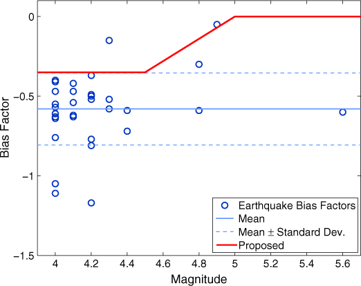
Distribution of calculated bias factors with mean and standard deviation indicated. The proposed bias factor curve is also indicated.

Figure 8 shows all of the station data for magnitude 4.0 and 4.2 Oklahoma earthquakes from 27 February 2010 to 20 June 2015 compared with predictions using Campbell (2003) with no bias, with the mean bias factor, and with the mean bias factor ± the standard deviation of the bias factors. Note that for magnitude 4.0 and 4.2 Oklahoma earthquakes, the mean bias factor plus one standard deviation is the proposed value. This figure also shows that even though the bias factors were fit to individual events, the mean of the bias factor still does a good job of fitting the data from all of the stations for a given magnitude. However, the figure also illustrates the considerable spread in the data. The biased model does not capture this amount of spread, so this model both underpredicts and overpredicts the extreme points. ShakeMap, however, is better able to reflect this spread because it analyzes real-time station data and includes these numbers in its S₁ calculations.

Figure 8.

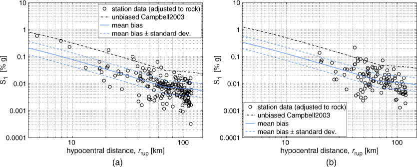
All station data for all earthquakes of magnitude (a) 4.0 and (b) 4.2 compared with predictions using Campbell (2003) with and without bias. Mean bias = −0.5803 and standard deviation = 0.2256.

Smart Inspection Radii

The spectral response accelerations predicted by the calibrated attenuation model presented in the preceding section represent the geometric mean of the horizontal components of S₁, not the maximum response in the horizontal plane, for hard rock (Site Class B) sites. For the purpose of determining inspection radii, the spectral accelerations computed from the biased Campbell (2003) model are first scaled by a factor of 1.30 to increase the motions to the maximum response (ASCE 2010, Beyer and Bommer 2006). Then, a site amplification factor was used to correct the model for Oklahoma soil. The average shear-velocity down to 30 m ( $V_{s}^{30}$ ) is a standard metric used to classify site conditions. A USGS custom $V_{s}^{30}$ map of Oklahoma and the surrounding area showed that only Site Class C and D are present in Oklahoma (USGS 2010). To ensure the inspection radii were independent of the location of the earthquake, Site Class D (stiff soil) was used to represent all of Oklahoma because it is more conservative than Site Class C. (Note that Site Class D is the default site class per the ASCE 7–10 building code where “the soil properties are not known in sufficient detail” [ASCE 2010 11.4.2].) The Site Class soil amplification factors found in NEHRP Recommended Seismic Provisions (Building Seismic Safety Council 2009) were used. In summary, the following formula was used to calculated adjusted S₁ values for inspection radii:

S_{D 1} = 2.4 \times 1.3 \times S_{1}

(9)

where S₁ is the geometric-mean spectral acceleration at 1.0 s for Site Class B and S_D1 is the maximum spectral acceleration at 1.0 s adjusted for site class effects (Site Class D).

Figure 9 shows the proposed attenuation relation for five magnitudes, assuming a depth of 5 km when calculating the hypocentral distance. This depth was selected because it is the average depth of Oklahoma earthquakes. These curves are then used to find an inspection radius for each magnitude based on the S₁ values selected from the base fragility curve (Figure 3). For each magnitude between 4.0 and 6.5, the largest radius at which the trigger S₁ (i.e., 0.0556 g) is expected to be exceeded was found. Figure 9a gives an example of this process: for an M5.0 earthquake, the proposed attenuation model shows that the inspection radius for a 25% probability of being in the slight damage state (S_D1 = 0.0556 g) is 13.1 km. Figure 9b shows the required inspection radii based on the biased Campbell (2003) model for magnitudes 4.5–6.5. To put the data in a format best suited for inspectors to use, the resulting radii were further grouped into “Smart Radii,” as shown in Figure 9b and presented in Table 2. The radii were converted from km to miles for inspection ease.

Figure 9.

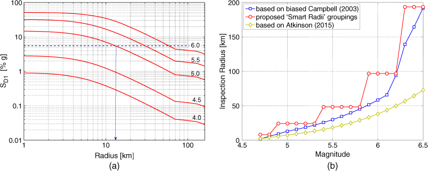
(a) Proposed attenuation model for magnitudes 4.0, 4.5, 5.0, 5.5, and 6.0, and selection of inspection radius for magnitude 5.0. (b) Comparison of magnitude-based inspection radii at which S₁ exceeds 0.0556 g.

Table 2

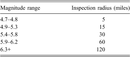
Proposed “Smart Radii” groupings

Magnitude range	Inspection radius (miles)
4.7–4.8	5
4.9–5.3	15
5.4–5.8	30
5.9–6.2	60
6.3+	120

Inspection Radii Validation

As noted in the Evaluation of Current Attenuation Models section, shallow small-to-moderate earthquakes may produce larger ground-motion amplitudes at short distances (Hough 2014, Gupta et al. 2017). Due to faster attenuation, the proposed model may under-predict the response at close distances, as shown in Figure 8a. To ensure that the proposed inspection radii are appropriate, they are compared with inspection radii determined from a recently proposed, improved attenuation model for induced-seismicity hazards (Atkinson 2015). The radii predicted by Atkinson (2015) are shown in Figure 9b. The minimum magnitude to produce a ground-motion amplitude of S₁ = 0.0556 g is M4.7 for both models. The inspection radii based on the proposed model are conservative (larger) compared with those based on Atkinson (2015) for all magnitudes except for M4.7 (1.6 and 2.0 km, respectively), but the “Smart Radii” grouping is conservative in this case (8.1 km). Therefore, the proposed inspection radii are appropriate.

As further validation of the proposed radii, the two bridges that were damaged during the M5.8 Pawnee earthquake were 24 and 11 km from the epicenter, which are both within the 30-mile (48.4-km) smart radius for a M5.8 earthquake (Table 2).

Interim Protocol

While the values presented in Table 2 were recommended to ODOT, they implemented a more conservative version of these radii. They changed the magnitude range to 4.4–4.7 for the five-mile inspection radius and to 4.8–5.3 for the 15-mile inspection radius, with all the other ranges remaining the same. DOTs are responsible for the safety of the traveling public, so an additional degree of conservatism was desired by the Department.

Application to other Emerging Seismic Regions

After developing a trigger value as previously recommended, other DOTs may apply this framework by (a) selecting an attenuation model for their area, (b) modifying the attenuation model to fit measured seismic data, and (c) combining the attenuation model and trigger value to determine inspection radii. This procedure is appropriate for those DOTs desiring to quickly establish a preliminary starting point for inspections. ShakeCast, described in the following section, offers a more refined inspection process, but requires additional setup and annual maintenance.

Developing Shakecast

The preceding development of the interim radius-based protocol is a preliminary approach to establishing a response plan in emerging seismic regions, but additional refinement is possible. This section takes the trigger value established for the development of the smart radii and uses it as a starting point for ShakeCast (Wald et al. 2008). ShakeCast (short for ShakeMap Broadcast) is a situational awareness application that automatically retrieves a ShakeMap from USGS, compares shaking intensities against users’ facilities’ fragility curves (Biasi et al. 2017), and sends email notifications of potential damage levels to responsible parties within 10–20 minutes. ShakeCast has the benefit of using real-time data to offer better ground motion estimates than using only an attenuation model. This helps overcome the limitations of current attenuation models (see Evaluation of Current Attenuation Models). However, the default attenuation model used for Oklahoma ShakeMaps (Atkinson and Boore 2006) does not account for differences in attenuation for induced earthquakes.

To create a ShakeCast instance, the recommended practices found in the Cloud Installation Guide were followed (USGS 2015a). Then, modifications of the standard fragility curves were made to better match Oklahoma's inventory, and these modified fragilities were used to populate the instance. Finally, the savings afforded by ShakeCast in terms of department of transportation resources are quantified through a few scenarios, in which ShakeCast is compared with the previous ODOT inspection radii and the smart radii.

Populating the Shakecast Database

In order to populate a ShakeCast instance, the files must be uploaded with information about the bridges and who should receive notifications about these bridges. The order in which the files are uploaded to ShakeCast is critical because notifications will not be sent if they are uploaded in the incorrect order. The order of these is Facility Inventory, User Groups, and, finally, User Inventory. The standard procedure, as outlined in the ShakeCast User Guide (USGS 2015c), was followed with a few modifications to meet ODOT's needs. One of these modifications was to create new facility types for each of ODOT's divisions (e.g., DIV1–DIV8). Another was the modification of the standard HAZUS fragility curves, as described in the next section. These fragility values, as well as other relevant bridge data, were automatically computed from ODOT's National Bridge Inventory (NBI) data and assigned to the Facility Inventory CSV (comma-separated values) file. The User Groups and User Inventory XML (Extensible Markup Language) files were generated by the ShakeCast Workbook (Q.-W. Lin, pers. comm., October 2016).

Fragility Curve Modifications

When calculating the fragility curves for ODOT's bridges, the standard HAZUS fragility curves were not appropriate in all cases. As previously mentioned, the slight fragility curve cannot be calculated prior to an earthquake. Because ShakeCast bridge inventories are uploaded prior to an earthquake, a trigger value is used instead. The same trigger value as previously described (i.e., a 1-s spectral acceleration of 0.0556 g) was assigned for the low (green) inspection priority threshold for every bridge in the inventory. In general, the moderate (yellow), moderate-high (orange), and high (red) inspection priority thresholds were set to the S₁ value corresponding to a 50% probability of moderate, extensive, and compete damage, respectively, per the HAZUS fragility curves. It is worth noting that there are certain bridge classes that are not represented in HAZUS, for example, masonry bridges and bridges with a variable skew angle. Therefore, to be conservative, the moderate, extensive, and complete median S₁ fragility values for these bridges were assigned to be 0.15, 0.20, and 0.25 g, which correspond to the lowest median fragility values calculated for ODOT bridges represented in HAZUS.

Another concern with the standard HAZUS fragility curves was that they do not take into account a bridge's actual condition at the present time. To account for this and be more conservative, two additional bridge properties were examined: (a) whether or not a bridge was fracture critical and (b) whether or not a bridge's superstructure or substructure were structurally deficient. The former is indicative of a bridge having at least one tension member whose failure will most likely cause a part of or the entire bridge to collapse and is identified by NBI item number 92A (FHWA 1995). The latter are identified by NBI item numbers 59 and 60, and for this study, an NBI rating of four or less in either category was deemed structurally deficient. For fracture critical and structurally deficient bridges, the moderate, moderate-high, and high inspection priority thresholds were set to the S₁ value corresponding to a 25% probability of damage from the HAZUS fragility curves. The purpose of this was to reduce the threshold values for these damage states so the threshold would be exceeded for lower levels of shaking.

Running Scenarios

To test ShakeCast and ensure that it was working properly, earthquake scenarios were run. The scenarios used were from previous Oklahoma earthquakes. Only two of the earthquakes Oklahoma has experienced to date (24 April 2017) had shaking levels high enough to trigger email notifications: the 6 November 2011 M5.7 Prague earthquake and the 3 September 2016 M5.8 Pawnee earthquake.

After a scenario has been triggered, one email is received per division affected. Each email has two parts: the body and an attached PDF. The body of the email includes a ShakeMap of the earthquake and a list of all affected bridges in the division. The PDF includes a map with the affected bridge locations from all divisions and a list of these bridges (Figure 10). This list included more detailed information about the bridges than in the email body. The information from these emails can be copied and pasted into Excel to be sorted such that division engineers can best organize a route to inspect bridges (a request of ODOT).

Figure 10.

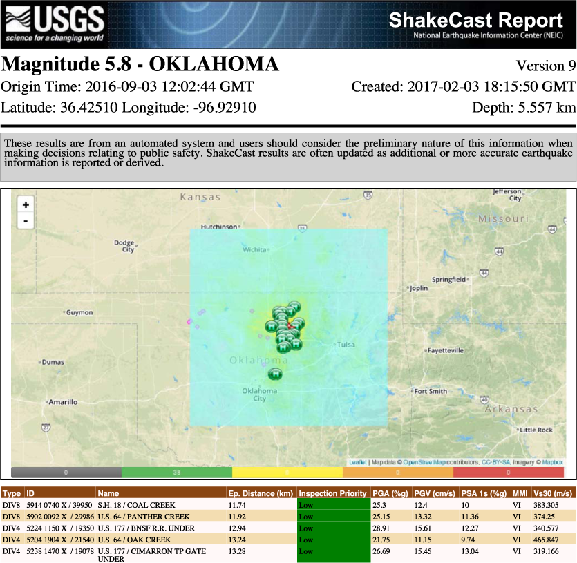
A screenshot from the emailed ShakeCast PDF.

Shakecast and Radii Comparison

By implementing ShakeCast, ODOT will be able to save money by reducing the number of bridges inspected. Figure 11 shows the number of bridges inspected using the old radii, the interim protocol, and ShakeCast for the M5.7 Prague and M5.8 Pawnee earthquakes. The average cost to inspect a bridge is $55 (W. L. Peters, pers. comm., 2016). This means that, using the interim protocol, about $32,000 would have been saved on the M5.7 Prague earthquake and about $11,000 was saved for the M5.8 Pawnee earthquake. Using Shakecast would have saved ODOT an additional $5,600 and $7,100 for each of the earthquakes, respectively. Additionally, ODOT will save money by inspecting for fewer earthquakes. For instance, in the year after the interim protocol was implemented (1 April 2016–31 March 2017), there were 13 earthquakes that would have required bridge inspections using the old protocol, four using the interim protocol (ODOT currently [24 April 2017] uses a modified version of the proposed smart inspection radii, which lowers the inspection threshold from M4.7 to M4.4), and only one using ShakeCast. This resulted in ODOT saving $15,700. Implementing ShakeCast over the same period would have saved an additional $8,800. In addition to the monetary savings afforded by the interim protocol and ShakeCast, the reduction in required inspections has raised the morale of inspection personnel that were experiencing fatigue due to the high number and frequency of unnecessary inspections.

Figure 11.

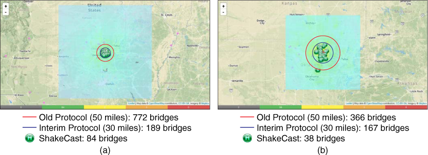
Comparison of the number of bridges to be inspected using the old radii, interim protocol, and ShakeCast for (a) the M5.7 Prague earthquake and (b) the M5.8 Pawnee earthquake.

Summary and Conclusions

Since 2009, there has been a dramatic increase in the number of earthquakes in Oklahoma. Therefore, concern has arisen about how Oklahoma's infrastructure will handle the increased seismic demand. In particular, ODOT is concerned about their bridges’ response to earthquakes and the potential for damage. To improve their earthquake response, ODOT implemented an interim protocol and then implemented ShakeCast. The first part of this study examined Oklahoma ground motions. Comparison of Oklahoma station data to the attenuation models found in the 2008 USGS seismic hazard map shows that most of the attenuation models overpredict Oklahoma ground motions; however, the Atkinson and Boore (2006) model has the best fit.

The smart inspection radii incorporated both the demand on and capacity of Oklahoma bridges. Demand was quantified by the ground-motion intensity, in this case spectral acceleration at a period of 1.0 s (S₁). Predictions of S₁ were made using the Campbell (2003) ground-motion attenuation model calibrated with a bias factor correlated to actual seismic station data in Oklahoma. These predictions were adjusted by a site amplification factor (Site Class D). Inspection radii were set to be the largest distance from the epicenter at which demand (S₁) exceeds capacity characterized by fragility curves of bridges. For the slight fragility curve, this capacity was set as a trigger value of 0.0556 g. Examining slight fragility curve values calculated for previous Oklahoma earthquakes showed that this trigger value is conservative.

The final step in preparing ODOT for the emerging seismic threat was the development of ShakeCast. To develop ShakeCast, HAZUS fragility curves were used with additional reductions for fracture critical, structurally deficient, and variable skew bridges. After populating the instance and running two scenarios, it was shown that ShakeCast recommends significantly fewer inspections than the inspection radii because it has better data on the ground shaking levels.

Other DOTs in emerging seismic regions may use this framework to help establish their own post-earthquake bridge inspection protocols. The level of desired conservatism can be established when determining the trigger value level of shaking. Then, the number of bridges to inspect can either be determined through inspection radii or ShakeCast, depending on the desired level of refinement.

Footnotes

Acknowledgments

This work was supported by the Oklahoma Department of Transportation (ODOT) under ODOT Engineering Contract EC-1609. Opinions, findings, and conclusions expressed in this paper are those of the authors and do not necessarily reflect those of the sponsoring organizations. The authors also acknowledge the technical advice of the ODOT Seismic Committee, in particular Steven Jacobi (ODOT), Walter L. Peters (ODOT), Gregg A. Hostetler (Infrastructure Engineers, Inc.), Karthik Radhakrishnan (Kleinfelder), and Zia Zafir (Kleinfelder).

References

American Association of State Highway and Transportation Officials (AASHTO), 2009. Guide Specifications for LRFD Seismic Bridge Design, Washington, D.C.

American Society of Civil Engineers (ASCE), 2010. Minimum Design Loads for Buildings and Other Structures, ASCE/SEI 7-2010, Reston, Virginia.

Atkinson

G. M.

2015. Ground-motion prediction equation for small-to-moderate events at short hypocentral distances, with application to induced-seismicity hazards, Bulletin of the Seismological Society of America 105, 981–992. doi:10.1785/0120140142.

Atkinson

G. M.

and Boore

D. M.

2006. Earthquake ground-motion predition equations for Eastern North America, Bulletin of the Seismological Society of America 96, 2181–2205. doi:10.1785/0120050245.

Basöz

and Mander

J. B.

1999. Enhancement of the Highway Transportation Lifeline Module in HAZUS. Tech. rep., National Institute of Building Sciences.

Beyer

and Bommer

J. J.

2006. Relationships between median values and between aleatory variabilities for different definitions of the horizontal component of motion, Bulletin of the Seismological Society of America 96, 1512–1522. doi:10.1785/0120050210.

Biasi

Mohammed

M. S.

and Sanders

D. H.

2017. Earthquake damage estimations: ShakeCast case study on Nevada bridges, Earthquake Spectra 33, 45–62. doi:10.1193/121815EQS185M.

Building Seismic Safety Council (BSSC), 2009. NEHRP Recommended Provisions for Seismic Regulations for New Buildings and Other Structures. FEMA

Washington, D.C.

Campbell

K. W.

2003. Prediction of strong ground motion using the hybrid empirical methods and its use in the development of ground-motion (attenuation) relations in eastern North America, Bulletin of the Seismological Society of America 93, 1012–1033. doi:10.1785/0120020002.

10.

Federal Emergency Management Agency (FEMA), 2003. Multi-hazard loss estimation method: Earthquake model: HAZUS MR4 technical manual. Washington, D.C.

11.

Federal Highway Administration (FHWA), 1995. Recording and coding guide for the structure inventory and appraisal of the nation's bridges. Office of Engineering Bridge Division FHWA-PD-96-001 edn.

12.

Frankel

A. D.

Mueller

Barnhard

Perkins

Leyendecker

Dickman

Hanson

and Hooper

1996. National Seismic-Hazard Maps: Documentation. Tech. Rep. 96-532, U.S. Department of the Interior, U.S. Geological Survey.

13.

Geotechnical Extreme Events Reconnaissance (GEER), 2016. The Geotechnical Aspects of the September 3, 2016 M5.8 Pawnee, Oklahoma Earthquake. Tech. rep.

14.

Gupta

Baker

J. W.

and Ellsworth

W. L.

2017. Assessing ground-motion amplitudes and attenuation for small-to-moderate induced and tectonic carthquakes in the central and eastern United States. Seismological Research Letters. doi:10.1785/0220160199. In press.

15.

Hough

S. E.

2014. Shaking from injection-induced earthquakes in the central and eastern United States, Bulletin of the Seismological Society of America 104, 2619–2626. doi:10.1785/0120140099.

16.

Keranen

K. M.

Savage

H. M.

Abers

G. A.

and Cochran

E. S.

2013. Potentially induced earthquakes in Oklahoma, USA: links between wastewater injection and the 2011 Mw 5.7 earthquake, Geology 41, 699–702. doi:10.1130/G34045.1.

17.

McGarr

Bekins

Burkardt

Dewey

J. P.

Earle

W. E.

Hickman

Holland

A. E.

Majer

J. R.

and Sheehan

2015. Coping with earthquakes induced by fluid injection, Science 347, 830–831. doi:10.1126/science.aaa0494.

18.

Owens

T. J.

Crotwell

H. P.

Groves

and Oliver-Paul

2004. SOD: standing order for data, Seismological Research Letters 75, 515–520. doi:10.1785/gssrl.75.4.515-a.

19.

Pacific Earthquake Engineering Research Center (PEER), 2015. NGA-East: Median Ground-Motion Models for the Central and Eastern North America Region. Tech. Rep. 2015/04, University of California, Berkeley, CA.

20.

Petersen

Moschetti

Powers

Mueller

Haller

Frankel

Zeng

Rezaeian

Harmsen

Boyd

Field

Chen

Rukstales

Luco

Wheeler

Williams

and Olsen

2014. Documentation for the 2014 update of the United States national seismic hazard maps. Tech. Rep. Open-File Report 2014-1091, U.S. Geological Survey.

21.

Petersen

M. D.

Frankel

A. D.

Harmsen

S. C.

and Mueler

C. S.

et al., 2008. Documentation for the 2008 Update of the United States National Seismic Hazard Maps. Tech. Rep. Open-File Report 2008-1128, U.S. Geological Survey.

22.

Petersen

M. D.

Mueller

C. S.

Moschetti

M. P.

Hoover

S. M.

Rubinstein

J. L.

Llenos

A. L.

Michael

A. J.

Ellsworth

W. L.

McGarr

A. F.

Holland

A. A.

and Anderson

J. G.

2016. 2016 One-Year Seismic Hazard Forecast for the Central and Eastern United States from Induced and Natural Earthquakes. Tech. Rep. Open-File Report 2016-1035, U. S. Geological Survey.

23.

Petersen

M. D.

Mueller

C. S.

Moschetti

M. P.

Hoover

S. M.

Shumway

A. M.

McNamara

D. E.

Williams

R. A.

Llenos

A. L.

Ellsworth

W. L.

Michael

A. J.

Rubinstein

J. L.

McGarr

A. F.

and Rukstales

K. S.

2017. 2017 one-year seismic-hazard forecast for the central and eastern United States from induced and natural earthquakes, Seismological Research Letters 88. doi:10.1785/0220170005.

24.

Robert

C. P.

and Casella

2004. Monte Carlo Statistical Methods. 2nd ed. Springer New York, NY.

25.

Shahjouei

and Pezeshk

2016. Alternative hybrid empirical ground-motion model for central and eastern North America using hybrid simulations and NGA-West2 models, Bulletin of the Seismological Society of America 106, 734–754. doi:10.1785/0120140367.

26.

Silva

Gregor

and Darragh

2002. Development of Regional Hard Rock Attenuation Relations for Central and Eastern North America. Tech. Rep. ML042310569, Pacific Engineering and Analysis, El Cerrito, CA.

27.

Somerville

Collins

Abrahamson

Graves

and Saikia

2001. Ground Motoin Attenuation Relations for the Central and Eastern United States. Tech. Rep. Award No. 99HQGR0098, U.S. Geological Survey.

28.

Tavakoli

and Pezeshk

2005. Empirical-stochastic ground-motion prediction for eastern North America, Bulletin of the Seismological Society of America 95, 2283–2296. doi:10.1785/0120050030.

29.

Toro

G. R.

Abrahamson

N. A.

and Schneider

J. F.

1997. Model of strong ground motions from earthquakes in the central and eastern North America: best estimates and uncertainties, Seismological Research Letters 68, 41–57. doi:10.1785/gssrl.68.1.41.

30.

U.S. Geological Survey (USGS), 2010. Custom

V_{s}^{30}

Mapping. Earthquake Hazards Program, archived version available at https://web.archive.org/web/20150518094331/http://earthquake.usgs.gov:80/hazards/apps/vs30/ (last accessed 18 June 2015).

31.

U.S. Geological Survey (USGS), 2015a. Cloud Installation Guide. ShakeCast V3.0, available at https://my.usgs.gov/confluence/display/ShakeCast/ShakeCast+V3.0 (last accessed 26 October 2015.

32.

U.S. Geological Survey (USGS), 2015b. Search Earthquake Catalogue. Earthquake Hazards Program, available at http://earthquake.usgs.gov/earthquakes/search/ (last accessed 30 June 2015).

33.

U.S. Geological Survey (USGS), 2015c. ShakeCast V3 User Guide. ShakeCast V3.0, available at https://my.usgs.gov/confluence/display/ShakeCast/ShakeCast+V3.0 (last accessed 10 November 2015).

34.

U.S. Geological Survey (USGS), 2016a. M 5.0 - 3km W of Cushing, Oklahoma. Earthquake Hazards Program, available at http://earthquake.usgs.gov/earthquakes/eventpage/us100075y8#executive (last accessed 22 December 2016).

35.

U.S. Geological Survey (USGS), 2016b. M 5.1 - 31km NW of Fairview, Oklahoma. Earthquake Hazards Program, available at http://earthquake.usgs.gov/earthquakes/eventpage/us20004zy8#executive (last accessed 28 November 2016).

36.

U.S. Geological Survey (USGS), 2016c. M 5.7 - Oklahoma. Earthquake Hazards Program, available at http://earthquake.usgs.gov/earthquakes/eventpage/usp000jadn#executive (last accessed 28 November 2016).

37.

U.S. Geological Survey (USGS), 2016d. M 5.8 - 14km NW of Pawnee, Oklahoma. Earthquake Hazards Program, available at http://earthquake.usgs.gov/earthquakes/eventpage/us10006jxs#executive (last accessed 28 November 2016).

38.

U.S. Geological Survey (USGS), 2016e. ShakeMap. Earthquake Hazards Program, available at https://earthquake.usgs.gov/data/shakemap/ (last accessed November 10, 2016).

39.

U.S. Geological Survey (USGS), 2017. Induced Earthquakes. Earthquake Hazards Program, available at https://earthquake.usgs.gov/research/induced/overview.php (last accessed 17 February 2017).

40.

Wald

D. J.

Lin

K.-W.

Porter

and Turner

2008. ShakeCast: automating and improving the use of ShakeMap for post-earthquake decision-making and response, Earthquake Spectra 24, 533–553. doi:10.1193/1.2923924.

41.

Worden

B. C.

Wald

D. J.

Allen

T. I.

Lin

Garcia

and Cua

2010. A revised ground-motion and intensity and interpolation scheme for ShakeMap, Bulletin of the Seimological Society of America 100, 3083–3096. doi:10.1785/0120100101.

42.

Zwillinger

1995. CRC Standard Matematical Tables and Formulae. CRC Press Boca Raton, FL.

A Framework for Post-Earthquake Response Planning in Emerging Seismic Regions: An Oklahoma Case Study

Abstract

Introduction

Seismicity in Oklahoma

History of Odot'S Post-Earthquake Inspection Protocol

Evaluation of Current Attenuation Models

Developing Interim Protocol

Determining Trigger S1 Value

Trigger Value Validation: Computing Slight Fragility Curve

Validation Using Seismic Station Data

Validation Using ShakeMap Grid Data

Application to other Emerging Seismic Regions

Modifying Campbell (2003) Attenuation Model

Smart Inspection Radii

Inspection Radii Validation

Interim Protocol

Application to other Emerging Seismic Regions

Developing Shakecast

Populating the Shakecast Database

Fragility Curve Modifications

Running Scenarios

Shakecast and Radii Comparison

Summary and Conclusions

Footnotes

Acknowledgments

References

Determining Trigger S₁ Value