
Abstract
This paper represents the third part of a series of four publications on response history analysis for new buildings. Three real-building examples designed to a prior version of the building code are chosen, having a range of target spectrum characteristics, tectonic settings, and structural systems to test the new procedure and document its appropriate implementation. This paper describes the process of determining both MCER spectra and scenario spectra for all three examples. It explores selection of appropriate recorded ground motions and the procedure for scaling and spectrally matching to a maximum direction spectrum. Global results such as drift and treatment of unacceptable response, and local results such as force-and deformation-controlled acceptance criteria checks, are shown for each example. Practical guidance is given on implementing response history analysis for engineers employing the new Chapter 16.
Introduction
Substantial changes to response history analysis in the NEHRP Provisions (FEMA 2015) have been completed, and are now under consideration for ASCE 7 Chapter 16, to incorporate an updated philosophy based on current research, consensus documents and expert opinion. This paper represents Part III of a series of four publications describing this development process. Greater detail of the new provisions can be found in Part I and Part II (Haselton et al. 2017a, 2017b) while a study of assumptions made in the provisions’ development can be found in Part IV (Jarrett et al. 2017). The issue team tasked with revising ASCE 7 Chapter 16, hereafter referred to simply as Chapter 16, sought to test the procedure using three example buildings. These buildings were analyzed by practicing structural engineers familiar with response history analysis. The purpose for these examples is to:
Test the procedure. The end users of Chapter 16 are ultimately practicing structural engineers, many of whom perform response history analysis using other documents such as PEER TBI, ASCE 41 and ASCE 7-10 (PEER 2010, ASCE 2006, ASCE 2010). It is therefore imperative that the new chapter be useable to practicing structural engineers and incorporate current best practice without discouraging the application of response history analysis. Identify unclear or ambiguous requirements. The shortcomings of new code language often surface only after a methodology is adopted. Testing the proposed provisions during the code development stage can expose issues early in the process and allow revisions to be made before the language is finalized. Benchmark and identify parameters requiring further study. Since all the example buildings are designed to a prior version of the building code, any discordant results between the proposed provisions and previous code benchmarks would expose either unintended conservatism or lack of conservatism. Such discrepancies could then be studied to help technically justify or refute the proposed changes. Establish a standard of practice. Response history analysis, more than other analysis procedures, requires a large degree of engineering judgment. As a result, a wide range of assumptions exist in all steps of the process, from ground motion selection to nonlinear modeling. Those unfamiliar with response history analysis will therefore find these examples a solid introduction, while those who regularly implement response history analysis will find them instructive on the new Chapter 16 methodology.
This paper steps through each example in a way similar to the process in which a real design would be undertaken; the building is designed through elastic analysis and acceptable behavior is then verified through nonlinear response history analysis. The elastic analysis step is required by Chapter 16 and is assumed to be satisfied for these examples by design to a prior version of the building code. The next steps of the process include taking site properties and modal characteristics of the structure and determining the seismic hazard, developing target response spectra, and selecting and modifying ground motions. Next or concurrently, an analytical model is constructed in software capable of representing nonlinear behavior using state-of-the-practice modeling techniques. The proposed acceptance criteria procedures of Chapter 16 are then applied to local and global results. Iteration is typically required in the actual design process when analyzed building behavior is unacceptable, or to search for an optimized solution, but is not employed as part of this study.
Example Buildings Overview
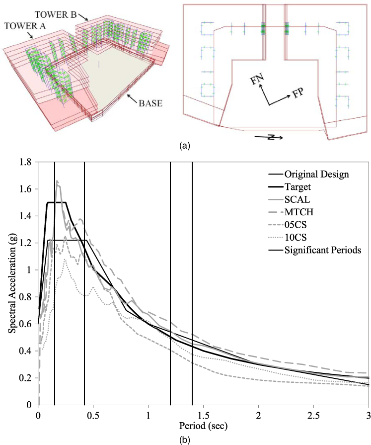
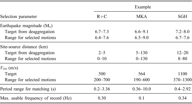
To implement the proposed procedure of Chapter 16, three example buildings are selected. The buildings are selected to represent a range of target spectrum characteristics, tectonic settings, structural systems and analytical software employed. Table 1 presents the formal selection criteria and defining characteristics for each example. The characteristics of the selected buildings intentionally span the range of parameters for which response history analysis using Chapter 16 is expected. Each team, comprising the authors from Rutherford + Chekene (R+C), Magnusson Klemencic Associates (MKA) or Simpson Gumpertz & Heger (SGH), respectively, create an example building based on a structure recently designed by their firm using elastic analysis techniques.
Example building selection criteria
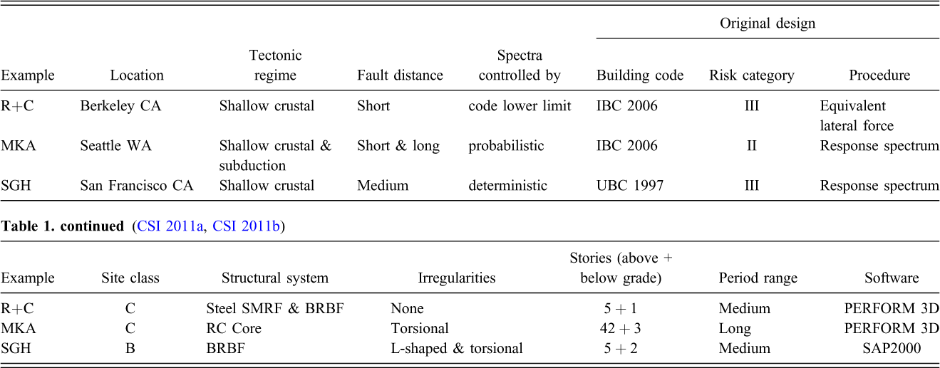
The first example, referred to as the R+C example, is located very close to the Hayward Fault in Berkeley, CA. Its site is thus subjected to both high seismicity and near-fault effects. Originally designed to the 2006 International Building Code (ICC 2006) as Occupancy Category III using the equivalent lateral force procedure, it employs a steel special moment-resisting frame (SMRF) in the longitudinal direction and buckling-restrained brace frame (BRBF) in the transverse direction as shown in Figure 1a. One story below grade relies on reinforced concrete perimeter walls with the remaining five stories of SMRF and BRBF appearing above grade level. The fault-normal and fault-parallel components of ground motion approximately align with the SMRF and BRBF directions, respectively, due to the north-south orientation of the Hayward fault. The R+C example is analyzed in PERFORM 3D (CSI 2011b).
(a) 3-D and plan views and (b) response spectra of R+C example.
Although Chapter 16 only requires one target spectrum and one suite of ground motions, or a minimum of two spectra and two suites when using the scenario spectra approach, multiple spectra and suites are analyzed for the examples presented in this paper. This provides a comparison between scaled versus spectrally matched motions and between uniform risk versus scenario spectrum procedures. Note that the original design spectrum of the R+C example is based on ASCE 7-05 (ASCE 2005) and closely matches the site-specific MCER target spectrum calculated for use in Chapter 16 (see Figure 1b). Figure 1b also shows the suite mean maximum direction spectrum for the SCAL, MTCH, 05CS, and 20CS suites, corresponding to ground motions either scaled to the uniform risk spectrum, spectrally matched to the uniform risk spectrum, scaled to a 0.5 s conditional spectrum, or scaled to a 2.0 s conditional spectrum, respectively. Suite mean is defined in this study as the arithmetic mean of a specified parameter over all ground motions within a suite. First and second mode periods in the SMRF direction are 1.7 s and 0.57 s with 72% and 10% mass participation factors, respectively, while in the BRBF direction the periods are 1.1 and 0.35 s with 71% and 13% mass participation factors, respectively. Mass participation factors include the mass of the ground floor.
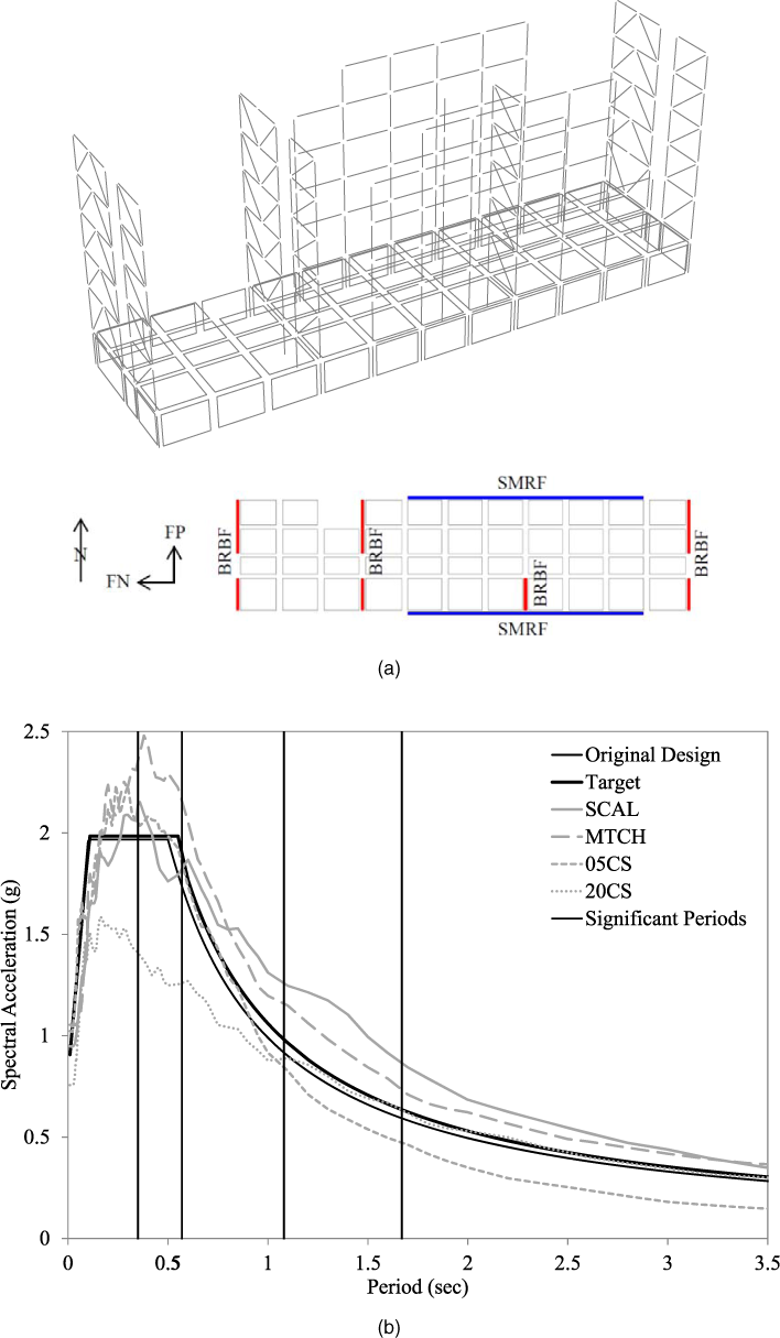
The MKA example, located in Seattle, WA, has significant contributions from both close/crustal and far/subduction-zone events while the seismic hazard for the site is probabilistically governed. The building was originally designed using the response spectrum procedure under the 2006 International Building Code (ICC 2006) as Occupancy Category II and rises 42 stories above grade with an additional three below. Its lateral system in the upper stories is composed of a core of reinforced concrete shear walls with some walls terminating at Level 33. Additional shear walls occur below Level 9 and perimeter basement walls exist below grade. The MKA example is analyzed in PERFORM 3D (CSI 2011b).
Figure 2b shows the site-specific MCER target spectrum developed for use in the Chapter 16 provisions along with the suite mean maximum direction spectrum for each of four suites: SCAL, MTCH, 10CS and 50CS. These correspond to ground motion suites scaled to the uniform risk spectrum, spectrally matched to the uniform risk spectrum, scaled to a 1.0 s conditional spectrum, or scaled to a 5.0 s conditional spectrum, respectively. First and second mode periods in the north-south direction are 3.9 s and 1.0 s with 59% and 17% mass participation factors, respectively, while in the east-west direction they are 4.6 s and 0.93 s with 58% and 21% mass participation factors, respectively. Due to the narrow concrete core, the building is torsionally irregular.
(a) 3-D and plan views and (b) response spectra of MKA example.
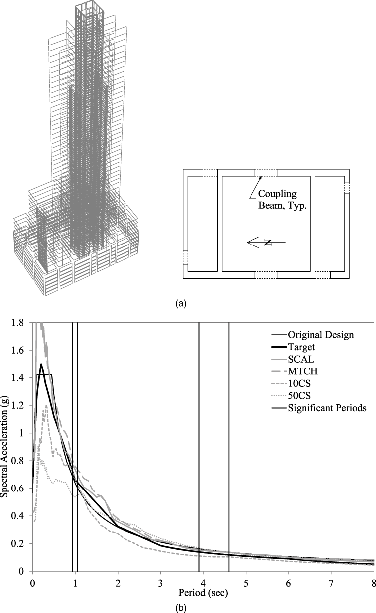
Lastly, the SGH example is located in San Francisco, CA. It was originally designed using the response spectrum procedure supplemented by limited linear response history analysis under the 1997 Uniform Building Code (ICBO 1997) for Occupancy Category III. Two torsionally irregular L-shaped, five-story towers of BRBFs sit atop a two-story podium supported by reinforced concrete walls, as shown in Figure 3a. Unlike the other two examples, the SGH example is analyzed in SAP2000 (CSI 2011a) to demonstrate that the Chapter 16 procedure is possible in multiple software platforms.
(a) 3-D and plan views and (b) response spectra of SGH example.
Figure 3b shows the suite mean maximum direction spectrum for the SCAL, MTCH, 05CS and 10CS suites, corresponding to ground motions either scaled to the uniform risk spectrum, spectrally matched to the uniform risk spectrum, scaled to a 0.5 s conditional spectrum, or scaled to a 1.0 s conditional spectrum, respectively. The significant modes of the torsionally irregular towers and base are at approximately 1.4 s, 1.2 s, 0.42 s, and 0.15 s with multiple modes of slightly different periods clustering around each period indicated. Due to the tower's irregular shape, translational and torsional modes are coupled. Mass participation factors, including the mass of the building's base level, are approximately 10% and 6%, 36% and 42%, 10% and 9%, and 24% and 19% in the north-south and east-west directions, respectively.
MceR Target Spectra
The MCER target spectra are developed based on the site characteristics for each example. MCER target spectra fall under Method 1 of Chapter 16. Although site-specific response spectrum procedures are not required, they are employed here to obtain a more accurate representation of the seismic hazard and ensure consistency between the two record selection methods considered. The following steps illustrate the method of ASCE 7 Chapter 21 (ASCE 2010) including consideration of deterministic and probabilistic hazard, adjustment for risk targeting, and treatment of maximum direction spectra. The procedure is illustrated in Figure 4 for the R+C example (other examples follow a similar process but with different values).
Step 1: Determine Probabilistic Spectra
Compute site-specific geometric mean uniform hazard spectrum (UHS): This is obtained from the USGS deaggregation tool (USGS 2008) based on site location, VS30 and a return period of 2,475 years or, equivalently, a 2% probability of exceedance in 50 years. Adjust geometric mean to maximum direction UHS: The geometric mean spectrum of Step 1a is multiplied by the period-dependent maximum direction scale factors of ASCE 7 Section 21.2 (ASCE 2010). Note that this step may be omitted if a maximum direction UHS is computed directly. Adjust UHS to uniform risk spectrum (URS): The maximum direction uniform hazard spectrum of Step 1b is multiplied by the period-dependent risk coefficients of ASCE 7 Section 21.2.1.1 (ASCE 2010). Note that one could also adjust from UHS to URS through iterative integration of the hazard curve with a collapse fragility curve per ASCE 7 Section 21.2.1.2.
Step 2: Determine Deterministic Spectra
Compute site-specific maximum direction deterministic spectrum: This is constructed based on the 84th percentile spectral values for the controlling fault. If the ground motion prediction equations used to compute the 84th percentile values for the controlling fault predict geometric mean, then the resulting spectrum must be adjusted by the maximum direction scale factors (e.g., see Step 1b above). Adjustment for risk-targeting (i.e., Step 1c above) does not apply to deterministic spectra. Compute transition spectrum: This is constructed based on a code-shape spectrum having S
s
of 1.5, S1 of 0.6 and corresponding site amplification factors, F
a
and F
v
. It is often referred to as the transition spectrum since it tends to geographically transition between deterministically-controlled and probabilistically-controlled sites. Define deterministic spectrum: The deterministic spectrum is the larger of the spectrum from Steps 2a and 2b.
Step 3: Determine Lower Limit Spectrum
Compute lower limit spectrum: The MCER spectrum constructed per ASCE 7 Section 11.4.5 and 11.4.6 (ASCE 2010) for the site is multiplied by 80% to define a lower limit on the site-specific values.
Step 4: Determine Target Spectrum
Define MCE
R
target spectrum - The MCER target spectrum used in design is taken as the period-by-period minimum of the probabilistic (Step 1c) and the deterministic (Step 2c) but not less than the lower limit (Step 3).
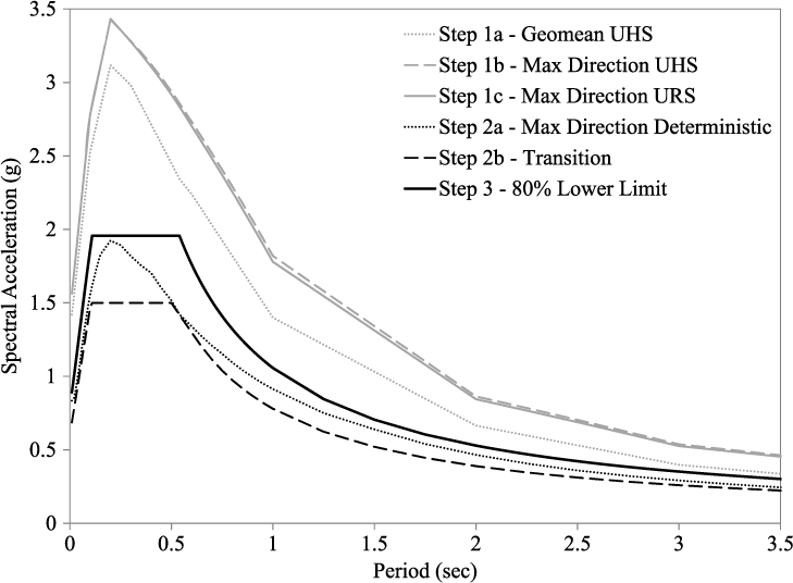
Example creation process of site-specific MCER target spectrum of the R+C example.
For the R+C example, it is clear from Figure 4 that the site's seismic hazard is deterministically governed. This is expected due to the structure's close proximity to a fault capable of large magnitude earthquakes. The MCER target spectrum at all periods ends up being controlled by the lower limit of 80% of the ASCE 7 Chapter 11 spectrum (i.e., Step 3 controls). In contrast, the MCER target spectrum for the MKA example is probabilistically governed for almost the entire period range (i.e., Step 1c controls). Additionally, the MCER target spectrum for the SGH example is set by the transition spectrum (i.e., Step 2b controls) for most periods but is also governed by the probabilistic (i.e., Step 1c controls) between periods of approximately 0.25 s and 0.75 s.
Scenario Target Spectra
In addition to MCER target spectra, scenario target spectra for each of the examples are developed. Scenario spectra recognize the fact that a uniform hazard spectrum is controlled by different earthquake “scenarios” at different periods. Scenario spectra therefore intend to reduce conservatism by quantitatively deconstructing uniform hazard spectrum into a finite number of scenario spectra. The scenario spectra in this study are developed in accordance with the requirements of Chapter 16 Method 2 using the conditional mean spectrum (CMS) approach (Baker 2011).
To start, two or more conditioning periods for each structure are identified by observing the structural modes with the most significant mass participation. Then a CMS is constructed such that the spectral ordinate at all other periods represents the expected value given that the value at the conditioning period matches the MCER. Since the R+C example is for a deterministically governed site, the conditional spectra are determined manually using the controlling magnitude and distance, and computing the 84th percentile spectral acceleration for that event at the conditioning period. For the other sites, the USGS CMS tool (USGS 2008, Lin et al. 2013) is used to find a CMS with spectral amplitude closest to the target MCER at the conditioning period. Some minor scaling of the resulting spectrum is then performed to provide an exact match to the MCER at the conditioning period.
Per Chapter 16, the envelope of the scenario spectra must exceed 75%of the target MCER for all periods within the period range of interest. In these examples, the 75% floor tended to be reached near the extreme ends of the period range of interest and thus it was deemed preferable to increase the controlling scenario spectrum at those periods, rather than add scenario spectra, to satisfy this requirement. Figure 5 illustrates this for the R+C example. If the range of periods over which the 75% floor controlled became more significant, it may be necessary to add an additional scenario spectrum. Figure 5 shows the 05CS and 20CS conditional spectra suites developed using the above outlined approach for the R+C example. The 05CS and 20CS target spectra have conditioning periods of 0.5 s and 2.0 s to capture first and second modes of response, respectively. Note that although the 20CS target spectrum falls below the 75% floor at the lower end of the period range of interest, it does not need to be increased because the 05CS target spectrum exceeds the 75% floor.
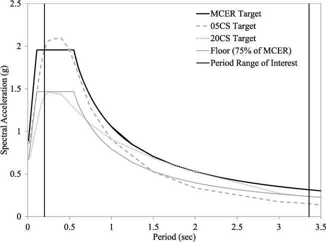
Example scenario target spectra for the R+C example.
It should be noted that this methodology illustrates one way to satisfy the Chapter 16 Method 2 requirements. However, it is by no means the only acceptable approach. Another alternative would be to compute median spectra for the dominant magnitude/distance scenario associated with the MCER spectrum at each conditioning period, and then scale those spectra to the MCER amplitude. Similar guidance appears in nuclear industry documents (U.S. Nuclear Regulatory Commission 1997).
If the CMS is the chosen basis for development of scenario spectra, several tools are currently available to facilitate the calculations (USGS 2008, EZ-FRISK, PEER n.d.). It is anticipated that additional applications will automate large portions of this process by the time Chapter 16 becomes an enforced standard.
Ground Motion Selection and Modification
Regardless of whether the target spectra are MCER or scenario based, eleven ground motion time histories are selected for each spectrum and grouped to form a suite. Each motion is chosen for consistency with the target spectrum as described below. Both horizontal ground acceleration components, represented in the fault-normal and fault-parallel orientations, are used. Vertical ground acceleration is not considered in this study.
The PEER (Chiou et al. 2008) and KiK-Net (Okada et al. 2004) ground motion databases are screened for each example independently based on several criteria. Table 2 summarizes the target values and chosen ranges. The criteria to select ground motions are shown below. Greater detail on the justification for each criterion can be found in the Part I companion paper (Haselton et al. 2017a). Note that not all the criteria below are strict requirements of Chapter 16 but generally represent either the authors’ opinion on best practice or current approaches in use.
Tectonic environment and rupture mechanism. Ground motions are taken from the tectonic environment in which the example's site is located. The R+C and SGH examples occur in shallow crustal regions, so ground motions from subduction zone events are excluded from their suites. Since the MKA example is exposed to both shallow crustal and subduction zone events, ground motions from both tectonic environments are included. Within a tectonic environment, all rupture mechanisms (e.g., strike-slip, normal, reverse, etc.) are permitted.
Magnitude and distance. The controlling magnitude and distance are taken from the hazard deaggregation for each site. Records with magnitude and distance within a range around these controlling values are permitted in order to obtain a sufficient number of potential ground motions.
Site class. Soil conditions are known for each example's site from geotechnical investigations. Ground motions recorded where soil conditions are more than one site classification away from the actual example's site are excluded. For example, the R+C example is located in Site Class C so only Site Class B, C and D ground motions are permitted.
Scale factor. Ground motions are not allowed to be scaled by less than 0.25 or more than 4 from their as-recorded amplitudes. This criterion is relaxed for subduction zone motions for the MKA example in order to obtain a sufficient number of ground motions.
Number of recordings per event. No more than three recordings from any one earthquake event are used in any ground motion suite. This criterion is again relaxed for the subduction zone events. When more than one recording is taken from a single event, it is recommended to check for uniqueness by observing their location relative to another and to the fault, and the similarity of their acceleration time series.
Pulse characteristics. Each suite for the R+C example (near-fault site) is checked to ensure several ground motions with pulse characteristics are included. A similar check is performed for the shallow crustal records for the MKA example while no such check is made for the SGH example.
Ground motion selection criteria. Note that the presented ranges envelope the ranges of all suites considered for the given example (e.g., SCAL,05CS, etc.). These ranges can be much tighter for individual ground motion suites
Each potential ground motion is scaled to match the target spectrum on average over the period range of interest (see Figure 6a). The sum of squared errors between the logarithm of the target spectrum and logarithm of the scaled motion's spectrum over the period range of interest is then computed. The eleven motions which fulfill all of the selection criteria with the smallest sum of the squared errors are chosen as a ground motion suite. It is also checked whether the suite mean spectrum exceeds 90% of the target spectrum at all periods. Note that the target spectra in Chapter 16 are maximum direction. The ground motion spectra must therefore also be maximum direction to ensure a meaningful scaling procedure. All maximum direction ground motion spectra for these examples are calculated directly from the acceleration time histories.
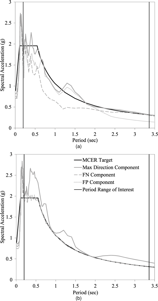
Response spectra for the same ground motion (a) scaled to the MCER and (b) spectrally matched to the MCER.
The above procedure is applied to produce suites where the ground motions are scaled to the target spectrum; these suites are denoted SCAL in this paper when the target is the MCER spectrum and CS when the target is a scenario spectrum. Chapter 16 also permits spectrally matched suites under certain, more restrictive conditions. To create these suites (e.g., MTCH suites), the individual ground motion components from the SCAL suite were spectrally matched to the target spectrum (Hancock et al. 2006). Note that since both components are being spectrally matched to the target spectrum, the resulting maximum direction spectrum will always meet or exceed the target (see Figure 6b). This intentionally places a penalty on the use of spectral matching under Chapter 16. Further detail on the penalty applied to spectral matching can be found in the companion papers (Haselton et al. 2017a, Jarrett et al. 2017). The resulting scaled and spectrally matched suite mean spectra for each example can be found in Figures 1b, 2b, and 3b. While it is recognized that free-field, as-recorded ground motions are independent of the structure being analyzed, the dynamic characteristics of the structure are important (via the period range of interest) in selection and modification to meet the target spectrum.
R+C Analysis & Results
Analytical Model
A three-dimensional (3-D) analytical model of the R+C example is constructed in PERFORM 3D (CSI 2011b) taking into account building geometry, expected gravity loading, suitable restraint conditions, P-Delta effects, inherent viscous damping, and appropriate element stiffness for such phenomena as concrete cracking and steel panel zone flexibility. While the upper floors are constrained as a rigid diaphragm, the first-floor diaphragm flexibility is modeled explicitly as required by Chapter 16 because of the significant change in story stiffness between the frames above and concrete walls below. Structures with vertical discontinuities and horizontal irregularities may also require such diaphragm modeling. The ground motions are applied at the lowest level of the R+C example and direct modeling of soil-structure interaction (SSI) is not employed. At the time of this writing, accidental torsion is not included in the nonlinear response history analysis step of Chapter 16 and is therefore neglected for the R+C Example.
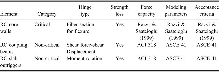
Component actions for each structural member are categorized based on their ability to reliably accommodate ductility demand (deformation-controlled) or inability to do so (force-controlled). Furthermore, both deformation- and force-controlled actions are divided into subgroups based on the consequence of exceeding a deformation or force level, respectively. These subgroups, listed in order of decreasing consequence of exceedance, are entitled critical, ordinary and non-critical. Table 3 presents a summary of the element modeling and component action designations for the deformation-controlled structural members of the R+C example.
Deformation-controlled component modeling for R+C example
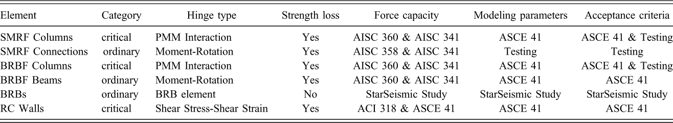
Chapter 16 does not intend to define plastic displacement limits or hinge models for every type of deformation-controlled structural component and material but rather takes the approach of providing a framework through which test data or other resource documents can be interpreted. For example, the hinge model for BRBF beams for the R+C example is taken from ASCE 41 (ASCE 2006) and the acceptance criteria are translated from ASCE 41 terminology into an appropriate value for use in Chapter 16. It must be emphasized that nonlinear response history analysis models and results should be extensively verified through elastic analysis, subassembly models and other simplified methods to ensure intended versus actual model behavior.
Global Results
In terms of global criteria, Chapter 16 contains two provisions. The first involves a process of identifying and accounting for an unacceptable response. Depending on the risk category of a structure and the type of ground motion suite selected (i.e., scaled versus spectrally matched), one unacceptable response may be permitted. Although an unacceptable response is not allowed by Chapter 16 for the R+C example because it is Risk Category III, the procedure for addressing an unacceptable response is presented here for demonstration purposes.
In Figure 7, a single ground motion from the 05CS suite produces drift significantly larger than the rest of the suite. It can be classified as an unacceptable response per Chapter 16 based on the fact that the steel moment frame hinges have exceeded their valid range of modeling. Applying the procedure for the occurrence of an unacceptable response results in the suite “mean” story drift being redefined as the larger of the mean of the remaining ten motions or 1.2 times the median of the full suite. If no unacceptable response had occurred, the suite mean story drift would have been simply the mean of the full suite. A similar calculation would need to be performed on local responses of deformation- and force-controlled components. Note that even though the unacceptable response is flagged as excessive drift in the SMRF direction, all results including those in the BRBF direction are affected. For example, suite mean story drifts in the BRBF direction must also be taken as the larger of the mean of the remaining ten or 1.2 times the median of the full suite despite the fact that the unacceptable response occurred in the SMRF direction.
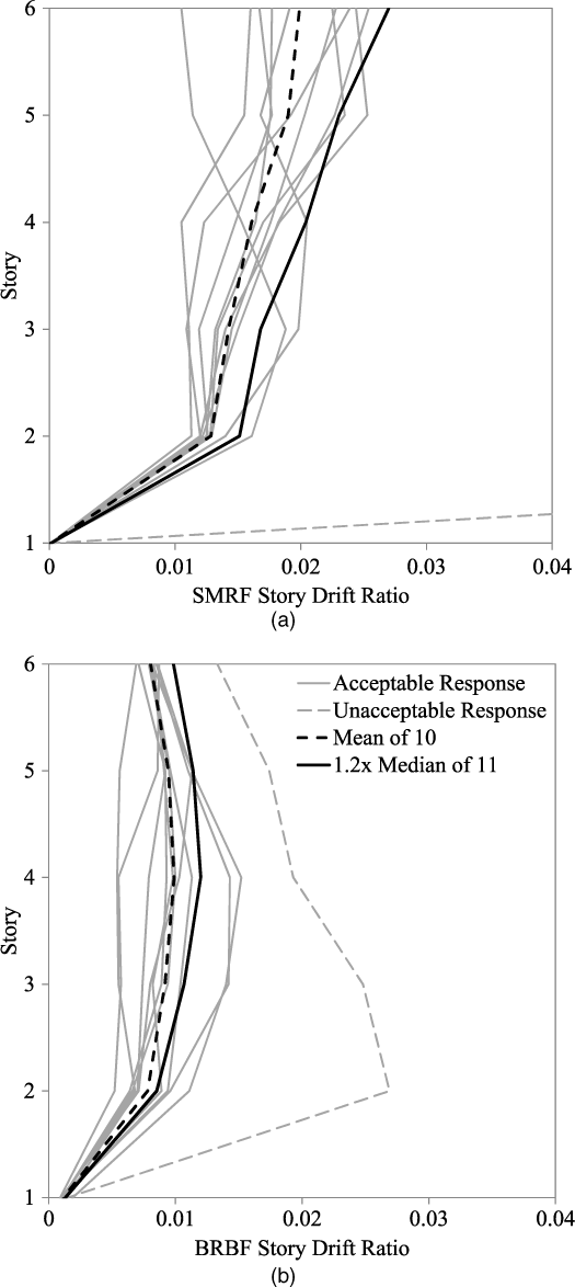
Story drift ratios of 05CS suite for (a) SMRF and (b) BRBF direction of R+C example showing how to handle case of one unacceptable response. Note that the unacceptable response motion produces drift ratios exceeding the plotted limits in (a).
The second global criteria in Chapter 16 concerns story drift. Chapter 16 modifies the drift limits in ASCE 7 Chapter 12 (ASCE 2010) to adjust for both maximum considered, rather than design basis, earthquake shaking and for an average ratio of response modification coefficient to deflection amplification factor (R/Cd). These adjustments have been substantiated fully in previous research (Uang and Maarouf 1994). Figure 8 shows the suite mean story drift ratios for the R+C example with results for the 05CS suite modified due to the unacceptable motion. Although provisions are under consideration in Chapter 16 for monitoring drift at the extreme edges of the building, all drifts for the R+C Example are computed at the building's center of mass. In general, the story drift profile is one indicative of a combination of first and second mode response. Note that the first story drift ratio is very small due to the large stiffness of the first story concrete walls compared to the SMRFs and BRBFs above. The first story drift ratio is greater in the BRBF direction due to both less concrete wall length and the contribution of diaphragm deflection. The conditional spectra suites (05CS and 20CS) tend to predict smaller drift ratios than either the SCAL or MTCH suites. This follows logically from the difference in fundamental approach between a MCER and a scenario target spectrum, namely that the scenario target spectrum approach does not require full combination of demand from all modes simultaneously. Keep in mind, though, that both the 05CS and 20CS suites must independently satisfy the Chapter 16 checks for a structure to be deemed compliant. Also important is the disparity between the SCAL and MTCH suites. The SCAL suite mean tends to exceed the MTCH suite mean in the SMRF direction and vice versa for the BRBF direction. This issue, which affects near-fault sites, is discussed in greater depth in Part IV (Jarrett et al. 2017).
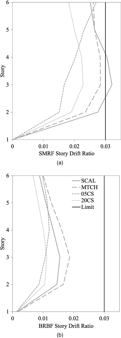
Suite mean (including unacceptable response provision) story drift ratios for (a) SMRF and (b) BRBF direction of R+C example. Drift limits also shown.
Local Results
Crucial to the definition of acceptance criteria for deformation-controlled actions in Chapter 16 is identification of the point at which a structural member is no longer capable of supporting its gravity load. Once this value is established (i.e., from test data or other resource documents) and the categorization of the structural member is completed (e.g., critical, ordinary, or non-critical), the Chapter 16 procedure defines a limiting displacement limit. As an example, the acceptance limit for a steel column would correspond to the plastic rotation at which gravity load could no longer be maintained. The ratio of the plastic rotation demand to the plastic rotation acceptance limit therefore becomes something of a demand-limit ratio (DLR), analogous to demand-capacity ratios used in linear procedures.
Figure 9 plots the percentage of deformation-controlled elements with a DLR meeting or exceeding a specified DLR versus that specified DLR for each of the four suites explored in the R+C example. Note that similar to results for story drift ratio, the 05CS and 20CS suites produce DLRs lower than the SCAL and MTCH suites. BRBF beams and columns and SMRF columns tend to be quite far from exceeding their acceptance limits, with one notable SMRF column under the SCAL suite at a DLR of approximately 1.0, while SMRF beams and buckling-restrained braces (BRBs) are slightly closer. Collectively, however, all local acceptance criteria are met for every suite.
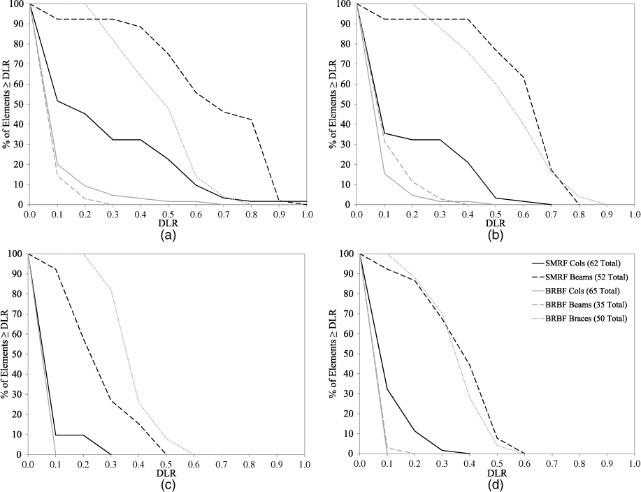
Suite mean (including unacceptable response provision) demand-limit ratios (DLRs) for deformation-controlled elements of (a) SCAL (b) MTCH (c) 05CS and (d) 20CS suites of R+C example. Reinforced concrete wall checks not shown.
Force-controlled element checks are not presented in detail in this study, however, portions of the lateral force-resisting system such as BRB gusset connections, panel zones of SMRF columns, etc. are checked as force-controlled actions using the plastic mechanism exception in Chapter 16. This exception allows actions which are limited by a well-defined mechanism (e.g., not shear in a reinforced concrete wall) to be designed for the forces corresponding to that mechanism rather than from the response history analysis.
Mka Analysis & Results
Analytical Model
A three-dimensional analytical model of the MKA example is constructed in PERFORM 3D (CSI 2011b) taking into account building geometry, expected gravity loading, suitable restraint conditions, P-Delta effects, inherent viscous damping, and appropriate element stiffness. Since the first several stories of the MKA example include perimeter reinforced concrete (RC) walls in addition to the building's central core of reinforced concrete walls, explicit modeling of diaphragms at these levels is necessary to meet the Chapter 16 provisions. All other floors have a rigid diaphragm constraint applied. To capture the outrigger action provided by the slab between the RC core walls and the exterior columns, representative concrete columns and effective slab widths are included. The ground motions are applied at the lowest level of the structure and direct modeling of soil-structure interaction (SSI) is not employed. Accidental torsion is also neglected.
Table 4 presents the deformation-controlled structural members for the MKA example. Force-controlled element actions include shear in diaphragms, shear in reinforced concrete walls and shear in reinforced concrete gravity columns.
Deformation component modeling for MKA example
Global Results
No unacceptable responses occur for the MKA example and the story drift ratios computed at the building's center of mass are less than the limits imposed by Chapter 16. In general, the story drift ratios increase with height, indicative of a flexure-type global response that is characteristic for shear walls (see Figure 10). Note that the story drift ratios grow more dramatically at Level 33 due to inelastic action. Even though the MKA example complies with ASCE 7 Chapter 12 (ASCE 2005) procedures, hinging occurs not only at the base, but also in upper stories because concrete compressive strength decreases, wall thicknesses are reduced, and several walls terminate at Level 33.
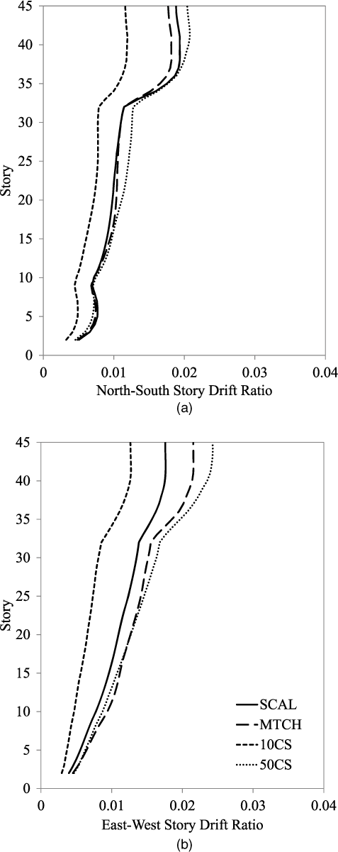
Suite mean story drift ratios in the (a) north-south direction and (b) east-west direction of the MKA example. Drift ratio limit of 0.04 not shown for clarity.
In contrast to the R+C example, one of the scenario spectrum suites (i.e., 50CS) generally produces story drift ratios which exceed the SCAL and MTCH suites. This is most evident in the east-west direction between the 50CS and SCAL suite mean story drift ratios and is likely a result of slight differences in the suite mean spectra near the fundamental mode period. The 10CS suite mean drift ratios are quite low since these motions do not excite the fundamental mode of the structure. Additionally, and likely owing to the fact that Chapter 16 imposes an intentional penalty on spectral matching, the MTCH suite mean story drift ratios tend to meet or exceed those of the SCAL suite.
Local Results
Local result conclusions for the MKA example mimic those for global results, namely that the demand-limit ratio (DLR) for deformation-controlled components is small. Although coupling beam rotation is also monitored, only compressive and tensile strains in the core walls are presented in Figure 11 for brevity. The inelastic action above Level 33 is especially evident. Also note that the qualitative differences in suite mean between ground motion suites for compressive and tensile strain are comparable to those for story drift ratio with the 50CS suite exceeding the others. Force-controlled element checks are not presented in detail in this study.
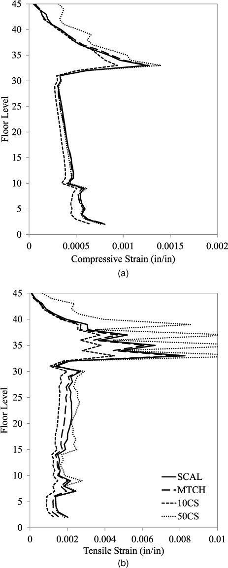
Suite mean strain in core wall in (a) compression and (b) tension for the MKA example. Strain limit of 0.003 (concrete in compression) and 0.05 (steel in tension) not shown for clarity. Note that the zig-zag behavior in the tensile strain diagram is a result of the strain monitoring method employed.
Sgh Analysis & Results
Analytical Model
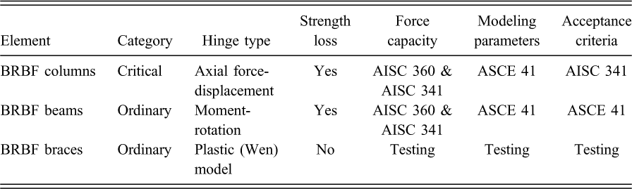
A three-dimensional analytical model of the SGH example is constructed in SAP2000 (CSI 2011a) using similar modeling techniques as for the R+C example except as noted below. Most notably, the BRBF columns were modeled with inelastic axial hinges. Although the preferred method would be to include axial-moment-moment (PMM) interaction hinges similar to those used for the R+C example, several of the authors have experienced difficulty with convergence when using PMM interaction in SAP2000. The intent of AISC 341 (AISC 2010b) for lateral force-resisting columns, however, permits the exclusion of axial-moment interaction for loading including amplified seismic loads. Note that if such a modeling technique is employed per AISC 341, as is done for the SGH example, columns are treated as deformation-controlled in tension and as force-controlled in compression. This is achieved by modeling axial behavior as inelastic with high ductility in tension and very low ductility in compression.
Since the force-controlled provisions of Chapter 16 are not applicable to inelastically modeled actions, the unacceptable response provisions instead define the acceptance criteria for columns in compression (whereby compressive inelastic axial behavior in a column is deemed unacceptable). Another approach, which was not explored in this example, is to model the columns as inelastic in tension but elastic in compression and use the deformation and force-controlled acceptance criteria, respectively, of Chapter 16. Table 5 displays the deformation-controlled components and their acceptance criteria for the SGH example.
Deformation-controlled component modeling for SGH example. Note that BRBF Columns are force-controlled in compression and deformation-controlled in tension. (
Global Results
In order to conform to the requirements of Chapter 16 as a Risk Category III structure, the SGH example is not permitted to have any ground motion produce an unacceptable response. However, one, zero, two and one unacceptable responses were observed for the SCAL, MTCH, 05CS and 10CS suites, respectively. A greater number of unacceptable responses for the SGH example as compared to the other examples is explained by the inclusion of inelasticity for force-controlled actions in BRBF columns. Inelastic compressive behavior in a column represents the point at which the compressive force demand exceeds its capacity, marking a point at which the column can no longer support axial load. With gravity loads explicitly included and only the lateral force-resisting elements modeled, instability occurs because a path for gravity load redistribution cannot be found analytically. This demonstrates an example of when the force-controlled component acceptance criteria in Chapter 16 shifts from the force-controlled provisions to the unacceptable response provisions.
Story drift ratios for the SGH example, computed at the extreme corners of each tower's diaphragm, are shown in Figure 12 and fall below the maximum target drift permitted by Chapter 16. This is expected for BRBFs which are typically strength, rather than drift, controlled. Similar to the R+C example, the scenario spectra suites (05CS and 10CS) produce smaller story drift ratios in both directions than the SCAL suite. Note that the MTCH suite exceeds the SCAL suite owing to the intentional penalty Chapter 16 imposes on spectrally matched ground motions.
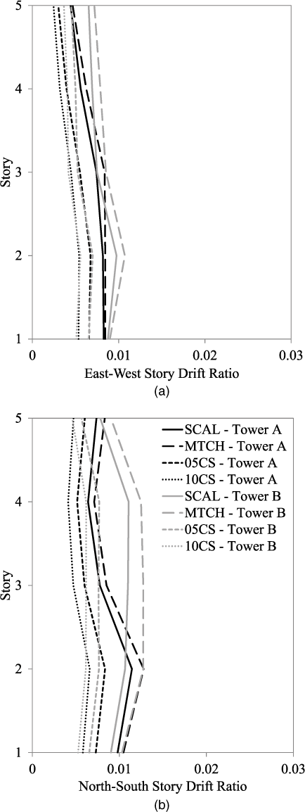
Suite mean (including unacceptable response provisions) story drift ratio for (a) east-west direction and (b) north-south direction of the SGH example. Although the 05CS suite resulted in two unacceptable responses, which is not permitted by Chapter 16, the unacceptable response provisions were applied to this suite anyway. Drift ratio limit of 0.03 not shown for clarity.
Local Results
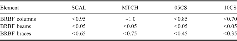
The deformation-controlled element demand-limit ratios (DLRs) for the SGH example are shown in Table 6. The relative DLRs for each structural member type between ground motion suites mimic the story drift ratios. In general, the MTCH suite results exceed the SCAL suite results and the scenario spectrum suites exhibit lower DLRs than either the SCAL or MTCH suites. Note that the DLR presented for the BRBF columns is only for axial tension. Axial compression is checked as force-controlled as described previously. Force-controlled element checks are not presented in detail in this study.
Deformation-controlled element demand-limit ratios (including unacceptable response provision) of SGH example. Although the 05CS suite resulted in two unacceptable responses, which is not permitted by Chapter 16, the unacceptable response provisions were applied to this suite anyway
Conclusions
The study of the three real-building examples during the revision of the NEHRP provisions (FEMA 2015) and ASCE 7 Chapter 16 helped produce provisions which are more consistent and implementable, and have been benchmarked against the current state-of-practice. In addition, these examples motivated several important changes which were incorporated during the Chapter 16 revision process:
Scenario spectra lower limit of 75% of MCE
R
: There was general agreement that the scenario target spectra should not fall below a certain percentage of the MCER target spectrum within the period range of interest, and it was through these examples that a practical limit was devised that balanced the requirement for more scenarios with the desire to not allow the scenario target spectra envelope to drop too low at any period. Spectral matching provisions: The examples generally verified that the Chapter 16 provisions impose a penalty on the use of spectral matching in terms of elastic response spectra, albeit in some cases (e.g., near-fault sites or when a scaled suite's suite mean exceeds the target due to record selection) this penalty is reduced or nonexistent. Furthermore, this penalty on the elastic response spectra does not translate linearly to global and local results. Period range of interest: Commentary was added to clarify that the 90% mass participation requirement in determining the lower bound of the period range of interest need not include the mass of stiff substructures. Unacceptable response provisions: The procedure for computing the suite mean response when an unacceptable response occurred was tested to ensure that it could not be “gamed” by arbitrary selection of an unacceptable motion. Story drift limits: Although the conversion from linear drift limits at the design-basis earthquake to nonlinear drift limits at the MCER has been previously documented in the literature (Uang and Maarouf 1994), the examples provided a technical basis on which the provisions could be founded.
Nonlinear response history analysis requires special expertise in all aspects of the process, from ground motions to analytical modeling to results interpretation. By illustrating the state-of-the-practice, these examples are intended to be instructive to practicing engineers on implementing the Chapter 16 methodology, and on benefitting from the insights nonlinear response history analysis can provide.
Footnotes
Acknowledgments
The work in this paper was completed in a subgroup of Issue Team Four, which was formed by the Building Seismic Safety Council's (BSSC) Provisions Update Committee. Travel and meeting expenses for Issue Team Four were partially funded by the Federal Emergency Management Agency (FEMA) of the Department of Homeland Security (DHS) through the BSSC. Additionally, the authors would like to recognize the financial and technical support of their respective firms: Rutherford + Chekene, Magnusson Klemencic Associates, and Simpson Gumpertz & Heger.