Hazard Disaggregation and Record Selection for Fragility Analysis and Earthquake Loss Estimation

Abstract

Economic losses and collapse probability are critical measures for evaluating the earthquake risk of existing buildings. In this context, this study sheds light on several problems and limitations in current practice of hazard-consistent ground-motion selection and fragility analysis, focusing on the impact that (commonly assumed) approximations in disaggregation outputs have on the aforementioned risk metrics, as opposed to an exact solution. These issues are investigated for several building classes, seismicity models and ground motion prediction equations (GMPE), for a site in the city of Lisbon (Portugal). It is observed that only an exact (i.e., rupture-by-rupture) disaggregation can lead to satisfactory results in terms of accuracy, when limit state criteria are not structure-specific. On the other hand, an approximate method is proposed, which still leads to statistically valid results regardless of the chosen structural class, seismicity model or GMPE.

Introduction

Earthquake-induced collapse and economic losses are critical measures for evaluating the earthquake risk of existing buildings, as well as assessing the effectiveness of risk reduction schemes (Liel 2008). As a result, such metrics must be as accurate as possible, appropriately reflecting the various sources of uncertainty associated with the evaluation of seismic risk. Otherwise, biased, unreliable or inadequate results may be achieved, resulting in ill-informed decisions.

With respect to seismic fragility and vulnerability, the largest source of uncertainty lies in the characterization of the input earthquake ground motion (Liel et al. 2009). Given a particular level of seismic intensity, these uncertainties are associated with several ground motion attributes that influence the designated “record-to-record” variability. Therefore, in this study we focus on the appropriate treatment of record-to-record variability in the context of fragility and vulnerability evaluation. In particular, we investigate what is the impact on earthquake loss estimations, when different degrees of accuracy are considered in the hazard-compatible ground motion selection for non-linear response history analysis.

A rigorous record selection approach requires both the determination of a “target” to compare the appropriateness of different ground motions, as well as an objective method for the selection, simulation and/or modification of ground motions to “match” this “target” (Bradley 2010). Several methodologies have recently been proposed in the literature, providing alternatives that allow the direct link between ground motion properties and PSHA. Among many studies, the conditional spectrum (CS), initially proposed by Baker and Cornell (2006) and further developed by Jayaram et al. (2011), provides the mean and variance of spectral ordinates conditioned on the occurrence of a specific value of a single spectral acceleration, as determined by PSHA. This method has its fundamental basis in the assumption that spectral accelerations follow a multivariate lognormal distribution. As hypothesized by Bradley (2010), this is not restricted to spectral accelerations, and can be extended to any arbitrary vector of ground motion intensity measures of interest (IM). As a result, the proposed general conditional intensity measure approach (GCIM) establishes that, for a given earthquake rupture (or scenario) discretized in the source model used in PSHA, a conditional vector IM has also a multivariate lognormal distribution.

According to the GCIM approach, considered in this study, an exact estimation of the “target” distributions of several intensity measures used for record selection and scaling shall be obtained as the contribution of all the possible (independent) ruptures influencing the hazard at a given site. As such, the contribution of each rupture conditioned on a particular level (of a given intensity measure) can be defined by seismic hazard disaggregation (Bazzurro and Cornell 1999). Because this “rupture-by-rupture” disaggregation is computationally demanding, it is not available as a standard output of most PSHA tools. Therefore, the simplification commonly used consists in grouping individual ruptures into “rupture scenarios” usually defined by a pair of causal magnitude (M)/distance (R). This approach is adopted in virtually all hazard disaggregation platforms. However, the impact of considering the hazard contribution of “rupture scenarios” (e.g., M/R intervals) in the computation of “targets” for record selection (e.g., Lin et al. 2013), as opposite to an exact “rupture-by-rupture” disaggregation, has been subject of limited scrutiny. More specifically, the level of error introduced by considering this approach instead of a more robust “rupture-by-rupture” disaggregation is still not clear.

In this study, the fragility, vulnerability, and loss assessment of nine distinct structural typologies is performed, using sets of ground motion records selected according to the GCIM approach. Target distributions are computed based on rupture contributions determined by seismic hazard disaggregation for Lisbon, Portugal; and several degrees of approximation are used, ranging from: (1) the exact consideration of all the possible ruptures contributing to hazard; to (2) a commonly used approach in which more coarse rupture scenarios are grouped into magnitude/distance bins. With respect to the latter, different M/R intervals are considered, in order to determine the level of error introduced by different approximations, as well as possible suitable levels of approximation recommended to be used by the research and practitioner communities. Furthermore, in this framework, distinct source models and ground motion prediction equations (GMPE) are considered, in order to assess how sensible the probabilistic loss estimation results are to the aforementioned approximations, when different GMPEs and seismicity models are used.

Structural Models

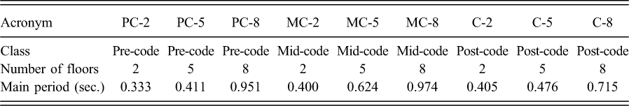
The numerical models considered herein correspond to the most typical class of buildings constructed in Portugal at different time periods: reinforced concrete (RC) structures with masonry infills. Drawing upon the study by Silva et al. (2014), in which material and geometrical properties of Portuguese building classes were characterized, statistical distributions of such properties have been used to create synthetic sets of 100 structures per building class; from which the numerical model corresponding to the median capacity has been selected, for each class. To account for the evolution of seismic design and its effect on seismic response, three different classes have been defined: pre-code, mid-code, and post-code. The first refers to buildings constructed before 1958 (i.e., previous to the publication of the first simplified seismic design code); mid-code buildings have been designed between 1958 and 1983 with a more rigorous code; and the last category includes structures built after 1983, time at which the modern seismic regulations were enforced in Portugal. In addition, three building heights per code class have been considered (two, five, and eight floors), leading to a total of nine different building classes (Table 1). Dynamic properties are characterized by the fundamental periods of vibration of the median structures obtained from random generation of 100 assets with varying geometrical and material properties. These have been found to range from 0.333 to 0.974 seconds, as presented in Table 1.

Table 1

Considered building classes and corresponding fundamental periods of vibration

Acronym	PC-2	PC-5	PC-8	MC-2	MC-5	MC-8	C-2	C-5	C-8
Class	Pre-code	Pre-code	Pre-code	Mid-code	Mid-code	Mid-code	Post-code	Post-code	Post-code
Number of floors	2	5	8	2	5	8	2	5	8
Main period (sec.)	0.333	0.411	0.951	0.400	0.624	0.974	0.405	0.476	0.715

To maintain the computational effort at a reasonable level, each structure is modeled as a single infilled moment frame with three bays. Each frame was modeled in a two-dimensional (2-D) environment using the open-source software OpenSees (2000), with force-based distributed plasticity beam-column elements. For the sake of synthesis, readers are referred to the aforementioned work by Silva et al. (2014) for details on the numerical considerations adopted with regards to the cross-sectional discretization and integration points of the elements, the material constitutive relationships, P-delta effects, the infill panel modeling, and applicable design provisions.

Methodology

The methodology implemented in this study consists of: (1) seismic hazard and disaggregation for the site of interest – Lisbon, Portugal; (2) record selection following the GCIM framework, compatible with the disaggregation results appraised in (1); (3) non-linear response history analysis (NLRHA) for the nine building models (one per building class) subjected to each set of records selected in (2); (4) fragility assessment for each building class and set of ground motion records resulting from distinct discretization methods used in disaggregation; and (5) seismic vulnerability and probabilistic loss estimation for each fragility model defined in (4).

Description of the Probabilistic Seismic Hazard Analysis Models

In order to account for the epistemic uncertainty associated with the definition of the seismicity in the area of interest, PSHA is performed based on four distinct source models. The first (referred herein as VF-model) has been obtained from the study of Vilanova and Fonseca (2007), in which the Portuguese seismic catalogue has been reviewed in order to define a new seismic zonation; whilst the remaining three have been developed within the FP7 SHARE project (Woessner et al. 2015). The latter includes an area source model (AS-model) based on the definition of areal sources for which earthquake activity is defined individually; a kernel-smoothed zonation-free stochastic earthquake rate model (Hiemer et al. 2014) that considers seismicity and accumulated fault moment (SEIFA-model); and a fault source/background seismicity model (FSBG-model), based on the identification of large seismogenic sources using tectonic and geophysical evidence (Haller and Basili 2011).

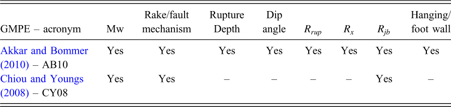
For consistency with the aforementioned studies, hazard and disaggregation calculations have been performed using the ground motion prediction equations (GMPE) of Akkar and Bommer (2010) and Chiou and Youngs (2008), separately, for each source model. These equations correspond to GMPEs to which the experts involved in the SHARE initiative attribute higher degree of confidence for application in the two tectonic environments applicable to Portugal: Active Shallow and Stable Continental Crust (Delavaud et al. 2012). The Authors acknowledge that the consideration of only two ground motion prediction equations is not sufficient to capture the effect of epistemic uncertainty in this region. However, the present objectives are: (1) to verify the impact of different attenuation relationships and corresponding set of rupture defining parameters in the computation of hazard-consistent fragility, for a given seismicity model; and (2) assess the influence of different seismicity models on the hazard-consistent fragility, when considering GMPEs with different degrees of detail in the definition of rupture properties (Table 2).

Table 2

List of rupture parameters in Akkar and Bommer (2010) and Chiou and Youngs (2008). R_rup is the closest distance to the rupture surface; R_x is the shortest horizontal distance to a line defined by extending the fault trace to infinity in both directions; and R_jb is the Joyner-Boore distance

GMPE – acronym	Mw	Rake/fault mechanism	Rupture Depth	Dip angle	R _rup	R _x	R _jb	Hanging/ foot wall
Akkar and Bommer (2010) – AB10	Yes	Yes	Yes	Yes	Yes	Yes	Yes	Yes
Chiou and Youngs (2008) – CY08	Yes	Yes	–	–	–	–	Yes	–

Seismic Hazard Disaggregation

Probabilistic seismic hazard analysis and disaggregation were performed using the OpenQuake-engine (Silva et al. 2014), in accordance with the theoretical background established by McGuire (2004) and Bazzurro and Cornell (1999), respectively. As a result, hazard disaggregation has been performed for the following rupture discretization approaches:

Rupture-by-rupture, that is, the contribution of all the independent ruptures generated by the earthquake rupture forecast (ERF) is computed, as illustrated in Figure 1.

Scenario ruptures, that is, the ruptures generated by the ERF are classified and grouped according to magnitude (M)/distance bins; assuming Joyner-Boore (R_jb) as the distance measure:

Magnitude interval (ΔM_w) = 0.2/Distance interval (ΔR_jb) = 2 km

ΔM_w = 0.4/ΔR_jb = 4 km

ΔM_w = 0.6/ΔR_jb = 8 km

ΔM_w = 0.8/ΔR_jb = 12 km

ΔM_w = 1.0/ΔR_jb = 20 km

With respect to methods 2a to 2e, one should note that evaluating the relative influence of increasing the interval of magnitude or distance individually is not the objective of this study. Differently, one is interested in determining the impact of using disaggregation methods with increasing approximation levels. As a result, the considered increase in magnitude intervals is proportional to that of distance.

Figure 1.

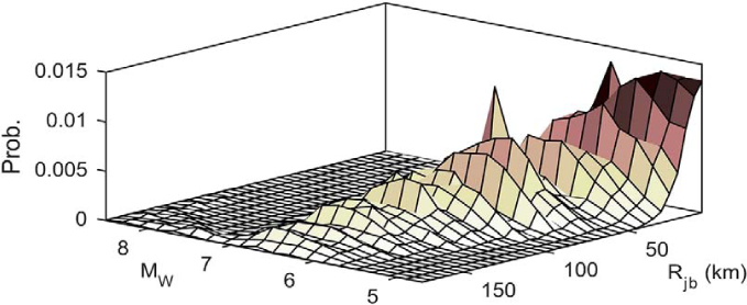
Rupture-by-rupture disaggregation (method 1), using the ERF generated for the FSBG-model, and Sa(T₁) = 0.5 g. Ruptures are grouped with ΔM_w = 0.2 ΔR_jb = 5 km, for visual clarity.

In addition, the parameters necessary for the application of the GMPEs cannot directly be obtained when methods 2a to 2e are used, because various ruptures are identified in each M/R_jb bin. Therefore, for each bin, the considered M and R_jb pair corresponds to the average values in the bin interval; whereas the remaining parameters (see Table 2) have been inferred from the rupture with higher disaggregation contribution to hazard. The OpenQuake-engine does not provide the contributions on a rupture-by-rupture basis. Instead, these are classified and grouped, as presented in 2). However, given the open-source nature of this tool, it was possible to produce the necessary intermediate results for the computation of P_{rup
_i
|
_IMj ^{= imj}} - the probability that the rupture properties are those of a particular rup_i, given that a ground motion (IM_j) has occurred, with an intensity of imj, as defined in Equations 1 and 2:

P_{r u p_{i_{|_{I M_{j} \geq i m j}}}} = \frac{\ln [1 - P_{I M_{j} \geq i m j_{|_{r u p_{i}}}}]}{\sum_{i = 1}^{I} v_{i} * P_{I M_{j} \geq i m j_{| r u p_{i}}}}

(1)

P_{r u p_{i_{|_{I M_{j} = i m j}}}} ≅ \frac{1}{v_{I M_{j} \geq i m j} - v_{I M_{j} \geq i m j + Δ i m j}} [P_{r u p_{i_{|_{I M_{j} \geq i m j}}}} . v_{I M_{j} \geq i m j} - P_{r u p_{i_{|_{I M_{j} \geq i m j + Δ i m j}}}} . v_{I M_{j} \geq i m j + Δ i m j}]

(2)

where I is the total number of ruptures in the ERF; v_i is the rate of occurrence of rup_i; v_{IM ≥ im} is the annual rate of exceedance of a ground motion with an intensity level of imj; and Δimj is a small increment of IM_j, relative to imj. As highlighted by Bradley (2010), Equation 2 becomes exact in the limit as Δimj → 0.

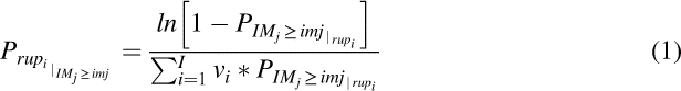
The parameters v_{IM_j ≥ imj} and v_{IM_j ≥ imj + Δimj} can directly be obtained from the standard outputs of the OpenQuake-engine hazard calculators. On the other hand, P_{IM_j ≥ imj_{|rup_i}} - the probability of IM_j being higher than a the level of interest im_j given a specific rupture rup_i – and the associated rate of occurrence v_i, can be retrieved using the “get_poes()” and “iter_rupturs()” functions, respectively. These are publically available on the Open-Quake-engine hazard library, referred to as “hazardlib” (GEM 2017).

Hazard-Consistent Record Selection

The GCIM approach is adopted herein for the purpose of record selection, as it allows the predictability (Kramer and Mitchell 2006) of all the intensity measures of interest. Readers are referred to the work of Bradley (2010) for a detailed description of the theoretical background of the methodology. In brief, the fundamental basis of the GCIM is that any set of ground motion parameters can be assumed to follow a multivariate lognormal distribution; and the conditional distribution given (1) a rupture scenario and (2) the occurrence of a specific value of IM_j, has a univariate lognormal distribution.

Upon definition of the ground motion prediction equation of interest and the correlation between the considered intensity measures, the conditional distribution of a certain intensity measure (IMi) given a level imj of a second intensity parameter (IMj) is given by:

f_{I M i_{_{| I M j = i m j}}} = \sum_{i = 1}^{I} f_{I M i_{| r u p_{i}, I M j = i m j}} . P_{r u p_{i | I M j = i m j}}

(3)

where f_{IMi
_{|IMj = imj}} is the probability density function (pdf) of IMi given IMj = imj; f_{IMi
_{| rup_i,IMj = imj}} is the pdf of IMi given IMj =imj and Rup = rup_i; and P _{rup_i | _{IMj = imj}} is obtained from disaggregation (methods 1 and 2a to 2e).

It shall be noted that, building on the mathematical formulation presented in Appendix E of the study by Baker and Cornell (2005), any of the methods 2a to 2e could potentially be used with little discrepancies in f _{IMi _{| IMj = imj}} (with respect to the exact method 1), provided that certain corrections are performed. More specifically, Equation 3, which accounts for the contribution of all the ruptures in the ERF, is equivalent to Equation 4, which simplifies Equation 3 by determining f _{IMi _{| IMj = imj}} as the weighted contribution of each disaggregation bin:

f_{I M i_{_{| I M j = i m j}}} = \sum_{k = 1}^{K} f_{I M i_{| b i n_{k}, I M j = i m j}} . P_{b i n_{k | I M j = i m j}}

(4)

where K is the total number of disaggregation bins; and f _{IMi _{| bin_k,IMj = imj}} and P _{bin_k _{| IMj} = imj} are determined as follows:

f_{I M i_{_{| b i n_{k}, I M j = i m j}}} = \sum_{j = 1}^{J_{k}} f_{I M i_{| r u p_{k}, I M j = i m j}} . P_{r u p_{j | I M j = i m j}}

(5)

P_{b i n_{k | I M j = i m j}} = \sum_{j = 1}^{J_{k}} P_{r u p_{j}_{| I M j = i m j}}

(6)

and J_k is the number of individual ruptures identified and grouped in bin k.

Knowing that both f _{IMi _{| bin_kIMj} = imj} and f _{IMi _{| rup_j,IMj} = imj} are lognormal probabilistic functions, a satisfactory approximation to the conditional mean and variance of f _{IMi _{| bin_kIMj} = imj} can be obtained by the first-order, second moment (Melchers 1999) method, as follows:

μ_{f}_{{_{I M i}}_{_{| b i n_{k}, I M j = i m j}}} = μ_{f_{I M i | \bar{M}, \bar{R_{J b}}} +} σ_{f_{_{_{I M i | \bar{M}, \bar{R_{J b}}}}}} . ρ_{\ln I M i, \ln I M j} . \bar{ε}

(7)

σ_{f}_{{_{I M i}}_{_{| b i n_{k}, I M j = i m j}}} = σ_{f_{I M i | \bar{M}, \bar{R_{J b}}}} \sqrt{1 - ρ_{\ln I M i, \ln I M j}^{2}}

(8)

where M , R _Jb , ε are the weighted mean of M, R_jb, ε (weights are the disaggregation probabilities of the J_k ruptures identified in the bin of interest – P_{rup_j _{| IMj} = imj}); and μ_{f _{IMi |
M
,
R
_Jb}}, σ_{f _{IMi |
M
,
R
_Jb}} are the mean and variance of f _IMi, respectively, evaluated at M , R _Jb .

Despite the possible advantages of this correction to methods 2a to 2e, a “rupture-by-rupture” disaggregation (method 1) would still have to be performed in order to identify each rupture probability (P_{rup_j _{| IMj} = imj}); therefore defeating the purpose of an approximate solution. For this reason, this approach was not addressed in this work. Differently, the present objective is to determine whether and at which degree of discretization an approximate approach such as 2a to 2e is able to provide accurate results in terms of fragility, vulnerability and loss, when compared with an exact solution (method 1).

“Targets” for Record Selection

The vector of intensity measures considered in this study (i.e., IM) includes intensity parameters (i.e., IMi) of peak ground acceleration (PGA), Housner intensity (HI) and spectral ordinates within the range of periods of 0.05 s to 3.0 s, conditioned on the spectral acceleration (IMj) at the mean fundamental period of vibration of each class – Sa(T₁); as thoroughly justified in Sousa et al. (2016). In the latter study, matters of predictability, efficiency (Shome and Cornell 1999), sufficiency (Luco 2002) and scaling robustness (Tothong and Luco 2007) have been verified when analyzing similar structural models. As recommended by Sousa et al. (2016), a number of 60 ground motion records have been selected and scaled per level of Sa(T₁), with the latter ranging from 0.1 g to 1.0 g, with intervals of 0.1 g.

The probabilistic distribution of the selected IM vector conditioned on a given level of Sa(T₁) is designated henceforth as f _{IM_|Sa(_T₁)=a}; being determined according to the hazard-consistent probabilistic distribution of each IMi given Sa(T₁) = a, as established in Equation 3, and the correlation models (between different intensity measures) enunciated in Sousa et al. (2016). For details regarding the database of natural ground motion records, readers are also referred to the study developed by Sousa et al. (2016). For the sake of illustration, the “target” probabilistic distributions of HI and spectral ordinates of periods ranging between 0.1 and 3.0 seconds are presented in Figure 2.

Figure 2.

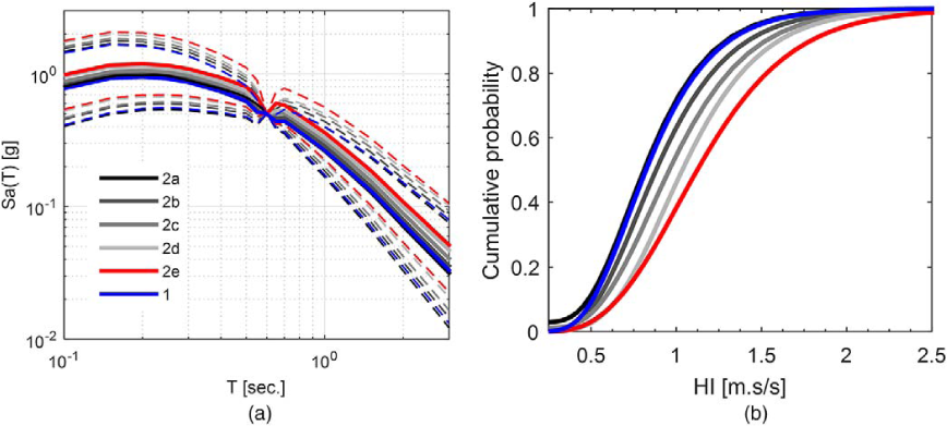
(a) Target spectral ordinates of periods ranging between 0.1 and 3.0 seconds (solid lines correspond to the mean and dashed lines represent 16 and 84 percentiles; i.e., mean +/−1 standard deviation); and (b) target cumulative probabilistic distribution functions of HI. In both cases, the results from disaggregation methods 1 and 2a to 2e (FSBG-model; CY08) are illustrated, considering a mid-code structure of five floors; for a conditional Sa(T₁) = 0.5 g.

In this figure, five-story (mid-code) structures are considered, and probabilistic distributions computed according to methods 1 and 2a to 2e are illustrated, in order to highlight the differences between hazard-consistent record-selection “targets” when different rupture discretization options are considered in hazard disaggregation. As illustrated in Figure 2, in which the FSBG-model and CY08 GMPE have been used, significant differences are verified between the mean of exact and approximate solutions, with discrepancies increasing proportionally to the increase of discretization interval. In other words, the accuracy of predictions decreases (and the bias increases) from method 2a to 2e, with respect to method 1. This increase in bias is associated with the approximation introduced by considering increasing intervals of magnitude and distance. As more thoroughly explained in the “Fragility comparison” section of this manuscript, the relative contribution of different magnitudes and distances “changes” with respect to the exact solution when moving from an exact to an approximate solution. Therefore, the results of approximate methods are biased with respect to exact method 1. In terms of variance, this discrepancy is reflected in the increase of uncertainty from method 2a to 2e, as verified in Figure 2b (i.e., the standard deviation of curve 2a is lower than that of 2e because curve 2a is “more vertical” than 2a). For the sake of synthesis, only a particular set of results are presented in Figure 2. However, similar differences in accuracy have been verified for each source model and GMPE investigated, for all the structures and levels of Sa(T₁).

A possible way to assess how differences in “targets” for ground motion selection propagate to discrepancies in fragility and loss results is to evaluate what is the degree of “similarity” between distributions of IMs in the resulting record sets. Therefore, in order to quantitatively compare conditional “target” distributions of IMs obtained from method 1 and 2a to 2e, a statistical approach was implemented. In this methodology, record sets selected based on approximate “target” distributions (from 2a to 2e) were individually compared with those obtained using method 1. For a given level of Sa(T₁) and building class (and a certain combination of source model/GMPE), one is able to evaluate what is the empirical distribution of each IMi (see the section Record Selection), for each set of records selected using methods 1 and 2a to 2e. Therefore, the null hypothesis that a given approximate empirical distribution follows the same underlying normal distribution as the corresponding exact one (method 1) can be assessed using the two-sample Kolmogorov-Smirnov (KS) test (Ang and Tang 2007).

For illustration, the p-values (Ang and Tang 2007) resulting from comparing the empirical distributions of Sa(T = 0.05 − 3.0 s) conditioned on Sa(0.624 s) = 0.5 g(MC-5) are presented in Figure 3, using the FSBG source model. For each T, the empirical distribution of Sa(T) obtained when records are selected for “targets” computed using methods 2a to 2e are individually compared with the those resulting from ground motions selected using the exact “target” distributions (method 1). In practice, one cannot reject the assumption of an approximate set of results being consistent with the exact method when the appraised p-value is higher than a specified significance level α. Based on these results (which are presented for each approximate method when compared with method 1, for each T), it is possible to recognize that p-values generally decrease from method 2a to 2e. In fact, these are lower than the selected significance level (α = 0.10) for methods 2b, 2c, 2d, and 2e, at least at one T instance, which implies that only in the case of method 2a the approximation is consistent with the exact method 1 (for α = 0.10).

Figure 3.

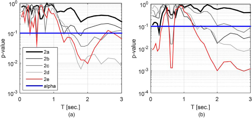
(a) p-values obtained with the KS test, when comparing empirical distributions of Sa(T₁ = 0.5 to 3.0 s) derived from records selected with approximate target distributions (methods 2a to 2e); as opposed to those obtained with the exact method 1. Conditioning Sa(T₁) = 0.5 g (MC-5), FSBG source model and AB10 GMPE. (b) Same as (a), but with CY08 GMPE.

As in the case of Figure 2, only a particular set of results are presented in Figure 3, for the sake of synthesis. Nonetheless, similar results have been attained for each combination of source model/GMPE investigated [as well as all structures and levels of Sa(T₁)]. More specifically, the assessed null hypothesis is systematically rejected for methods 2b, 2c, 2d and 2e; whereas method 2a tend to lead to “target” distributions that can be considered statistically identical to those referring to the exact method 1, at the 10% significance level.

The non-linear response of structures is a complex phenomenon that is influenced by ground motion properties that may not comprehensively be represented by the set of IMs considered herein. Therefore, the results presented in Figure 3, despite providing a valuable insight, care for appropriate validation through NLRHA and corresponding fragility and loss estimates.

Fragility and Loss Assessment

In the study herein, structural response is evaluated in terms of maximum inter-story drift (ISD) and global drift (GD) (i.e., maximum roof drift ratio), considering four damage states: Slight Damage (SD), Moderate Damage (MD), Extensive Damage (ED), and Collapse (Col). GD limits are determined according to the evaluation of structural capacity of each frame through a displacement-based adaptive pushover (Antoniou and Pinho 2004). As a result, displacement thresholds at each limit state are defined for each sampled frame without masonry infills (bare frame) according to the following assumptions:

Slight damage: Global drift at 50% of maximum base shear capacity.

Moderate damage: Global drift when 75% of maximum base shear capacity is achieved.

Extensive damage: Global drift at maximum base shear capacity.

Collapse: Global drift corresponding to a 20% decrease of the base shear with respect to maximum shear capacity, or 75% of the ultimate global drift attained in the pushover analysis, whichever is achieved first.

The influence of infill panels, which translates to a significant decrease of displacement capacity, is accounted for by applying the reduction factors proposed by Bal et al. (2010).

As thoroughly presented by Sousa et al. (2016), a fixed set of ISD values per limit state are defined based on the evaluation of global damage with increasing inter-story drift performed in real structures by Rossetto and Elnashai (2003). In order to adapt the six damage states proposed by the latter Authors with the one being considered in this study, light/slight damage and partial collapse/collapse damage states have been merged, as follows:

Slight damage: 0.08% maximum inter-story drift

Moderate damage: 0.30% maximum inter-story drift

Extensive damage: 1.15% maximum inter-story drift

Collapse: 2.80% or higher maximum inter-story drift

Fragility Comparison

For the purpose of fragility assessment, lognormal cumulative distribution functions have been fitted to the scatter of exceedance probabilities obtained for all the combinations of source model/GMPE. Based on the visual inspection of Figures 4 and 5, it is possible to conclude that, within each combination of source model/GMPE, the differences between approximate methods and method 1 tend to increase proportionally to the decrease of accuracy of the approximation (i.e., method 2a tends to lead to fragility curves that are “closer” to the those obtained with method 1; whereas method 2e is the one for which the differences with respect to method 1 are higher). However, these differences are not consistent across combinations of source model/GMPE; and are in fact exacerbated in the cases of AS and SEIFA source models (irrespective of the GMPE used).

Figure 4.

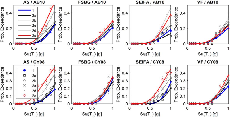
Fragility functions obtained with records selected based on methods 1 and 2a to 2e, for all the combinations of GMPE/source model. Limit state of Collapse using the ISD criteria; C-5 building class.

Figure 5.

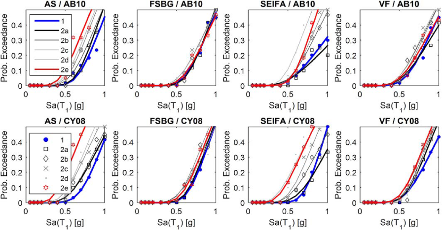
Fragility functions obtained with records selected based on methods 1 and 2a to 2e, for all the combinations of GMPE/source model. Limit state of Collapse (GD criteria); C-5 structural typology.

The degrees of discrepancy between approximate methods and method 1 verified in the case of AS and SEIFA models (versus those of FSBG and VF models) can be explained by the differences in the spatial distribution of possible independent events (and, more specifically, their magnitude), with respect to the site of interest. More specifically, as exemplified in Figure 6 for the case of methods 1 and 2c, it is possible to verify that the exact disaggregation results (method 1) indicate a much more homogeneous contribution across the investigated range of magnitudes and distances, in the case of the FSBG and VF models.

Figure 6.

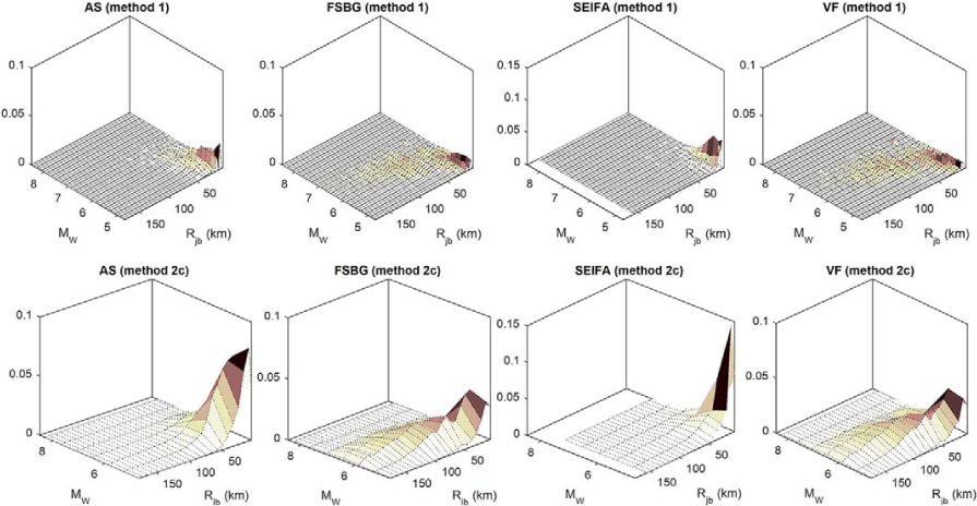
Disaggregation results for methods 1 and 2c, considering AB10 GMPE and the ERF generated for the AS, FSBG, SEIFA, and VF models; for Sa(T₁) = 0.5 g (C-5). Ruptures in the exact method 1 are grouped with ΔM_w = 0.1/ΔR_jb = 1 km, for visual clarity; and, in practice, contribution probabilities of method 2c result from aggregation of those of method 1 into coarser M, R_jb intervals.

On the other hand, the AS and SEIFA models’ disaggregation indicate a much more pronounced contribution of a limited range of small magnitudes and distances. For this reason, when hazard contribution probabilities are aggregated into more coarse M/R_jb intervals (as it happens when moving from method 1 to an approximate solution such as 2c) the distribution of probabilities across the M/R_jb range is altered much more significantly when the exact disaggregation results are clustered in a limited range of magnitude and distance (as in the case of the AS and SEIFA models). In fact, as visually depicted in Figure 6, the distribution of probabilities obtained with method 2c is very similar to that obtained with the exact method 1 for the case of FSBG and VF models. Differently, in the case of AS and SEIFA models, one can verify that the “spike” registered for low magnitudes and distances is much more pronounced in the case of method 2c than in method 1. As a result, as the discretization intervals increase (from methods 2a to 2e), the differences in disaggregation results increase more significantly when considering AS and SEIFA models. Consequently, the discrepancies between approximate and exact fragilities are also more significant in the case of AS and SEIFA models.

It shall additionally be mentioned that, in Figure 6, the C-5 building and Sa(T₁) = 0.5 g are selected for the sake of illustration. However, it has been verified that the trends exhibited here are common for all the structural classes and GMPEs used.

In addition, one might argue that non-negligible differences are also obtained between exact fragilities (method 1) across different combinations of source model/GMPE; which can be explained by the fact that the used intensity measure is not sufficient. In other words, because Sa(T₁) cannot comprehensively reflect all the ground motion properties influencing the seismic response of the assessed structures, fragility results are dependent on the ground motion properties of the selected set of records. Therefore, because different combinations of source model/GMPE provide different “targets” for selection (even for method 1), the exact fragilities are in fact distinct across combinations of source model/GMPE.

Given the wide range of seismic hazard modeling options evaluated, it would not be practical to present the comparison presented in Figures 4 and 5 for all the investigated building classes (and damage states). For this reason, only the results corresponding to the Collapse limit state of post-code five-story building (C-5) are illustrated. Nonetheless, it is noted that the illustrated differences are in fact representative of the results obtained for all the remaining structural typologies. The evaluation of the influence of these discrepancies is subsequently addressed by investigating what is the impact on the corresponding losses.

Vulnerability and Loss Estimation

In this section, vulnerability functions are drawn from the fragility curves presented above, using the consequence model adopted by Sousa et al. (2016) and Silva et al. (2014) in the evaluation of vulnerability of similar structural classes as those studied herein. As a result, damage ratios (ratio between cost to repair and total building value) of 0.1, 0.3, 0.6, and 1.0 are adopted for damage states SD, MD, ED, and Col., respectively. Although not presented for the sake of synthesis, fragility functions for limit states other than Collapse present similar scatter as those presented in Figures 4 and 5, as confirmed in Figure 7.

Figure 7.

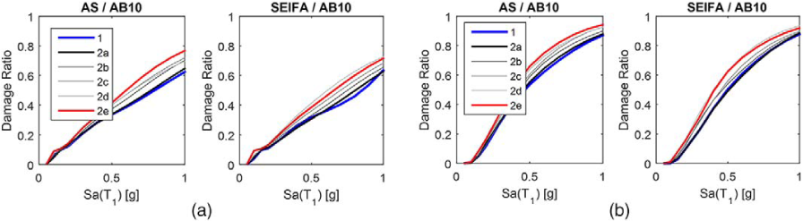
(a) Vulnerability functions obtained with records selected based on methods 1 and 2a to 2e, for AS/AB10 (left) and SEIFA/AB10 (right), combinations. ISD criteria and C-5 structural typology. (b) Same as (a), considering GD criteria.

In order to account for the propagation of uncertainty from fragility to vulnerability, the variability of damage ratios, for a specific level of Sa(T₁), is directly associated with the uncertainty in fragility regression. More specifically, 200 fragility functions are fitted to equal number of synthetic datasets randomly generated by bootstrap sampling with replacement (Wasserman 2004) from the original sets of intensity-specific probabilities. Because the bootstrapping is consistent across limit states (i.e., for a given simulation, the indexes of the probabilities sampled for SD are the same ones used to build the corresponding samples of MD, ED, and Col. probabilities), it is possible to compute a distinct vulnerability function for each bootstrapped fragility (Figure 8). As a result, loss exceedance curves are also computed for each of the bootstrapped vulnerability functions, for each method (1 and 2a to 2e), structural model and combination of source model/GMPE.

Figure 8.

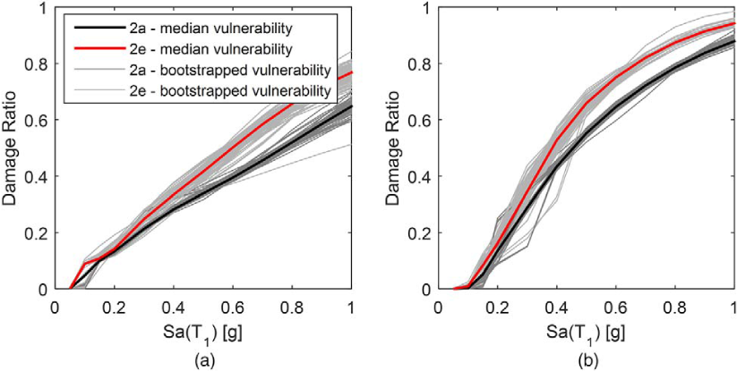
(a) Uncertainty in the vulnerability model obtained from bootstrapping with replacement from the original sets of damage exceedance probabilities. Structural typology of C-5, methods 2a and 2e, AS/AB10 combination, and ISD criteria. (b) Same as (a), considering GD criteria.

In this framework, the uncertainty in vulnerability is related with the uncertainty in fragility regression, which is further propagated into the estimation of loss exceedance probabilities. In other words, for a given building class and combination of source model/GMPE, one obtains 200 distinct loss exceedance curves, in accordance with the 200 bootstrapped vulnerability functions. For the purpose of comparing loss estimates obtained from approximate methods (2a to 2e) with those of method 1, average annual loss (AAL) values are computed for each of the bootstrapped loss exceedance curves. In this context, 200 independent AAL values are obtained for each disaggregation method, making it possible to compute 200 normalized differences between (1) AAL obtained with an approximate method (2a to 2e); and (2) AAL computed for method 1 (for each structural class and combination of source model/GMPE).

Using the sets of 200 AAL values, one could use statistical tests to compare distributions of (200) AAL values obtained with approximate and exact methods. However, because these results are obtained via bootstrap sampling, using statistical tests would not be a sound approach. More specifically, because the rejection of the null hypothesis (of the samples being drawn from the same distribution) is dependent on the sample size, it is possible to manipulate the number of bootstrap samples in order to reject or not the null hypothesis. As an alternative to comparing distributions of AAL from a statistical point of view, which would not be meaningful, it is possible to compute the probability that the difference between approximate and exact AAL values is higher than a specific threshold of interest. In the present case, the authors have decided that, based on our subjective judgment, an approximate method would be satisfactory if the resulting error is lower than 10%. Therefore, the suitability of each approximate method is herein evaluated as the probability of the attained error being higher than 10%, as shown in Figures 9 and 10. In these figures, only the results obtained when using AB10 GMPE are illustrated, since the magnitude of errors has been verified to be independent of the GMPE considered.

Figure 9.

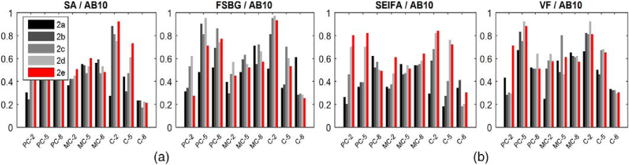
Probability of “Error” being higher than 10%; where “Error” is the absolute (normalized) difference between: (a) AAL obtained from methods 2a to 2e; and (b) AAL computed using method 1. Inter-story drift criteria and GMPE of AB10.

Figure 10.

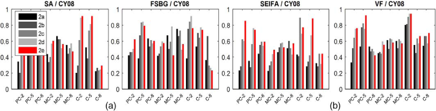
Probability of “Error” being higher than 10%; where “Error” is the absolute (normalized) difference between (a) AAL obtained from methods 2a to 2e; and (b) AAL computed using method 1. Global drift criteria and GMPE of AB10.

As illustrated, the probabilities of obtaining errors higher than 10% (herein simply referred as “error probabilities”) generally increase proportionally with the decrease in accuracy of the approximation (i.e., from method 2a to 2e), irrespective of the combination of source model/GMPE and structural class (more specifically, in approximately 80% of the assessed building class/source model/GMPE combinations).

Moreover, it was verified that such probabilities are significantly higher when ISD criteria are used to derive the fragility models (Figure 9), in comparison with the cases where GD criteria are considered (Figure 10). Several aspects may contribute to this discrepancy. ISD values are more significantly influenced by higher-mode effects than global drifts; which may lead to differences in the sufficiency of Sa(T₁) depending on which damage criteria is used. In addition, GD limit state thresholds are dependent on the properties of the sampled building (i.e., are directly derived from the assessed building capacity), whereas in the case of ISD the specified limits are obtained from experimental studies performed in similar structures. As a result, despite the fact that response parameters are obtained for the same sampled building in each class, there is a higher uncertainty introduced when limits are not building-specific. Similar conclusions regarding the effect of considering building-specific as opposite to building-independent damage criteria have been presented by Sousa et al. (2016). However, it shall be noted that definitive proof can only be provided by the analysis of four sets of damage criteria instead of two. More specifically, two sets of structure-specific and structure-independent criteria shall be compared, one for ISD and another using GD criteria.

Considering method 2a as the one for which an approximate approach generally imparts lower errors, Figure 11 presents the corresponding “error probabilities”, for all the combinations of source model/GMPE, and structural classes. As in Figures 9 and 10, the differences between results of ISD and GD criteria are evident. However, it is also possible to conclude that, despite the differences registered in fragility functions obtained for AS and SEIFA models (as opposed to FSBG and VF models; see the section Fragility Comparison), method 2a leads to “error probabilities” that do not exhibit a particular trend across source models (irrespective of the GMPE and structural model).

Figure 11.

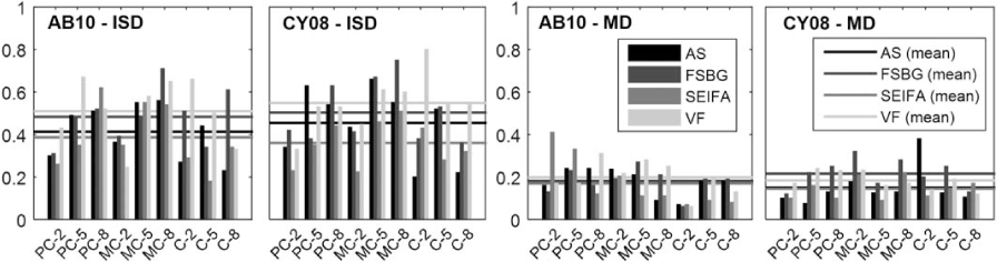
Probability of “Error” being higher than 10% obtained with method 2a; for all the combinations of source model/GMPE, structural classes, and limit state criteria. For clarity, horizontal lines correspond to the mean errors of all the structural classes, for each of the different source models.

This can be explained by the fact that, despite errors in fragility for a less accurate method (say, method 2e) are significantly higher in the case of AS and SEIFA models, method 2a provides the same level of approximation irrespective of the source model. More specifically, when GD criteria are used, an average “error probability” of approximately 20% is obtained; whereas average values of 50% are obtained for ISD. These results indicate that, for the structural classes and source model/GMPE combinations assessed, all the approximate dis-aggregation methods are inadequate when limit state criteria are not building-specific. On the other hand, when limit state thresholds are building-specific, method 2a constitutes a valid approximation, given the low value (20%) of probability of attaining errors higher than 10%.

Collapse Risk Assessment

In this section, risk estimates are further evaluated in the context of the collapse risk assessment of the buildings under scrutiny. For this purpose, the average annual probability of collapse has been determined and compared with limits prescribed by different authors and seismic design regulations. More specifically, the present objective is to evaluate the differences in “safety tagging” one would obtain by considering an approximate method, with respect to the exact probability of collapse. In this context, “safety tagging” is understood as the process of classifying a building's seismic safety, when comparing the appraised annual probability of collapse with the selected acceptable limits.

As presented in the study by Silva et al. (2016), in which the collapse probability of several building typologies has been assessed in order to determine the so-called “risk-targeted” hazard maps for Europe, ASCE (2010) establishes an acceptable risk of 1% in 50 years (approximately 2.0 × 10⁻⁴ annually) for the territory of the United States. On the other hand, Douglas et al. (2013) has adopted a value of 1.0 × 10⁻⁵ annually as a reasonable limit, following the literature review of several studies in which the annual probability of collapse of a number of structures designed according to modern regulations in France was determined.

Given the difference between the two proposals, both values (2.0 × 10⁻⁴ and 1.0 × 10⁻⁵) are considered herein for completeness, as boundary limits. For illustration, Figures 12 and 13 present the average annual probability of collapse for the mid-code and post-code buildings (for methods 1 to 2e), as well as the selected limits, for the AS/AB10 combination.

Figure 12.

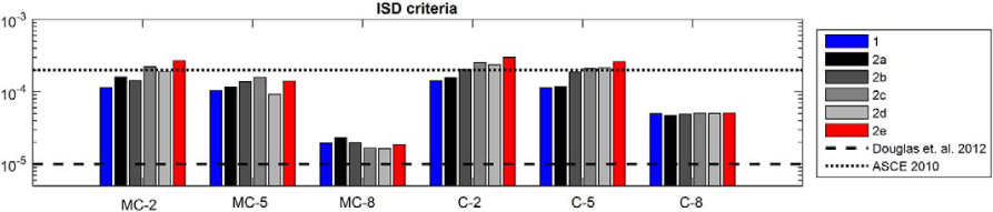
Average annual collapse probability (mid-code and post-code buildings) computed using methods 1 and 2a to 2e; for the AS/AB10 combination and ISD criteria.

Figure 13.

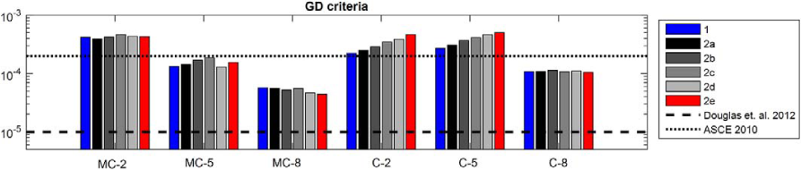
Average annual collapse probability (mid-code and post-code buildings) computed using methods 1 and 2a to 2e; for the AS/AB10 combination and GD criteria.

It is possible to verify that, for both limits of acceptable risk, method 2a leads to similar “safety tagging” as that obtained with the exact method 1, for both ISD and GD criteria. For the sake of synthesis, the results of pre-code structures are not illustrated, since the corresponding collapse probability values are systematically higher than 2.0 × 10⁻⁴, for all the methods (1 to 2e). In addition, only the AS/AB10 combination is illustrated; however, similar results (in terms of difference in “safety tagging” between exact and approximate methods) were verified for the remaining source models/GMPE.

Conclusions

In this study, hazard-consistent ground motion selection and fragility assessment were performed for nine building classes representing existing structures in Portugal. Target distributions for record selection were computed based on rupture contributions determined by seismic hazard disaggregation for Lisbon, Portugal; and several degrees of accuracy are used, ranging from: (1) the consideration of all the ruptures contributing to hazard; to (2) a magnitude (M)/distance (R_jb) bins.

In order to account for the epistemic uncertainty associated with the definition of seismicity in the area of interest, PSHA was performed using four distinct source models and two different GMPEs, with the objective of: (1) verifying the impact of different attenuation relationships and corresponding set of rupture defining parameters in the computation of hazard-consistent fragility; and (2) assessing the influence of different ground motion models on the hazard-consistent fragility, when considering GMPEs with different degrees of detail in the definition of rupture properties.

Based on the corresponding risk results evaluated in terms of AAL, it was verified that only an exact disaggregation method (i.e., contribution of all the possible independent ruptures) guarantees a satisfactory outcome in terms of accuracy, when using ISD criteria (which are structure-independent), irrespective of the source model/GMPE combination used. On the other hand, when using GD criteria, an approximate method in which magnitude/distance bins are defined with ΔM/ΔR_jb equal to 0.2/2 km (designated here as method 2a) generally lead to approximation results that are herein considered satisfactory (for the structures, source models, GMPEs, and site investigated herein). However, when the risk metric investigated is the annual probability of collapse, method 2a tends to provide appropriate results, irrespective of building class, source model, GMPE and limit state definition criteria.

This study demonstrated the possible advantages and limitations of considering approximate solutions to the problem of hazard-compatible record selection and subsequent analytical fragility and loss assessments; demonstrating that only an exact rupture-by-rupture disaggregation can unequivocally guarantee appropriate results. However, within the wide range of structural properties, response parameters, seismological source modeling options, and ground motion prediction equations assessed, recommendations have been provided regarding suitable levels of approximation to be used by the research and practitioner communities.

References

Akkar

, and Bommer

, 2010. Empirical equations for the prediction of PGA, PGV and spectral accelerations in Europe, the Mediterranean region and the Middle East, Seismological Research Letters 81, 195–206.

Ang

, and Tang

, 2007. Probability Concepts in Engineering: Emphasis on Applications in Civil and Environmental Engineering, John Wiley & Sons, New York.

Antoniou

, and Pinho

, 2004. Development and verification of a displacement-based adaptive pushover procedure, Journal of Earthquake Engineering 8, 643–661.

American Society of Civil Engineers (ASCE), 2010. Minimum Design Loads for Buildings and Other Structures, ASCE 7–10, Reston, VA.

Baker

, and Cornell

, 2005. Vector-Valued Ground Motion Intensity Measures for Probabilistic Seismic Demand Analysis, The John A. Blume Earthquake Engineering Center, Stanford, CA.

Baker

, and Cornell

C. A.

, 2006. Spectral shape, epsilon and record selection, Earthquake Engng Struct. Dyn., doi:10.1002/eqe.571.

Bal

, Crowley

, and Pinho

, 2010. Displacement-Based Earthquake Loss Assessment: Method Development and Application to Turkish Building Stock, IUSS Press, Pavia, Italy.

Bazzurro

, and Cornell

, 1999. Disaggregation of seismic hazard, Bulletin of the Seismological Society of America 89, 501–520.

Bradley

, 2010. A generalized conditional intensity measure approach and holistic ground-motion selection, Earthquake Engng Struct. Dyn., doi:10.1002/eqe.995.

10.

Chiou

, and Youngs

, 2008. An NGA model for the average horizontal component of peak ground motion and response spectra, Earthq. Spectra 24, 173–215.

11.

Delavaud

, Cotton

, Akkar

, Scherbaum

, Danciu

, Beauval

, Drouet

, Douglas

, Basili

, Sandikkaya

, Segou

, Faccioli

, and Theodoulidis

, 2012. Towards a ground-motion logic tree for probabilistic seismic hazard assessment in Europe, J. of Seismology, doi:10.1007/s10950-012-9281-z.

12.

Douglas

, Ulrich

, and Negulescu

, 2013. Risk-targeted seismic design maps for mainland France, Natural Hazards 65, 1999–2013, doi:10.1007/s11069-012-0460-6.

13.

GEM, 2017. 01 07. Openquake hazardlib, available at http://docs.openquake.org/oq-hazardlib/0.12/_modules/openquake/hazardlib/.

14.

Haller

, and Basili

, 2011. Developing seismogenic source models based on geologic fault data, Seis. Res. Let. 82, 519–525, doi:10.1785/gssrl.82.4.519.

15.

Hiemer

, Woessner

, Basili

, Danciu

, Giardini

, and Wiemer

, 2014. A smoothed stochastic earthquake rate model considering seismicity and fault moment release for Europe, Geophys. J. Int. 198, 1159–1172, doi:10.1093/gji/ggu186.

16.

Jayaram

, Lin

, and Baker

, 2011. A computationally efficient ground-motion selection algorithm for matching a target response spectrum mean and variance, Earthquake Spectra 27, 797–815, doi:10.1193/1.3608002.

17.

Kramer

, and Mitchell

, 2006. Ground motion intensity measures for liquefaction hazard evaluation, Earthquake Spectra 22, 413–438.

18.

Liel

, 2008. Assessing the Collapse Risk of California's Existing Reinforced Concrete Frame Structures: Metrics for Seismic Safety Decisions, Ph.D. Thesis, Stanford University.

19.

Liel

, Haselton

, Deierlein

, and Baker

, 2009. Incorporating modeling uncertainties in the assessment of seismic collapse risk of buildings, Structural Safety 31, 197–211.

20.

Lin

, Harmsen

, Baker

, and Luco

, 2013. Conditional spectrum computation incorporating multiple causal earthquakes and ground3motion prediction models, Bulletin of the Seismological Society of America 103, 1103–1116.

21.

Luco

, 2002. Probabilistic Seismic Demand Analysis, Connection Fractures, and Near-Source Effects, Ph.D. Thesis, Stanford University.

22.

McGuire

R. K.

, 2004. Seismic Hazard and Risk Analysis, Earthquake Engineering Research Institute, Oakland, CA.

23.

McKenna

, Fenves

, Scott

, and Jeremic

, 2000. Open System for Earthquake Engineering Simulation (OpenSees), Pacific Earthquake Engineering Research Center, University of California, Berkeley.

24.

Melchers

, 1999. Structural Reliability Analysis and Prediction, John Wiley, New York.

25.

Rossetto

, and Elnashai

, 2003. Derivation of vulnerability functions for European-type RC structures based on observational data, Engineering Structures 25, 1241–1263.

26.

Shome

, and Cornell

, 1999. Probabilistic seismic demand analysis of nonlinear structures, Technical Report RMS-35, RMS Program, Stanford, CA.

27.

Silva

, Crowley

, and Bazzurro

, 2016. Exploring risk-targeted hazard maps for Europe, Earthquake Spectra 32, 1165–1186, doi:10.1193/112514EQS198M.

28.

Silva

, Crowley

, Pagani

, Monelli

, and Pinho

, 2014. Development of the Open-Quake engine, the Global Earthquake Model's open-source software for seismic risk assessment, Natural Hazards, doi:10.1007/s11069-013-0618-x.

29.

Silva

, Crowley

, Pinho

, Varum

, and Sousa

, 2014. Investigation of the characteristics of Portuguese regular moment resisting frame RC buildings and development of a vulnerability model, Bulletin of Earthquake Engineering, doi:10.1007/s10518-014-9669-y.

30.

Sousa

, Silva

, Marques

, and Crowley

, 2016. On the treatment of uncertainties in the development of fragility functions for earthquake loss estimation of building portfolios, Earthquake Engineering and Structural Dynamics 45, doi:10.1002/eqe.2734.

31.

Tothong

, and Luco

, 2007. Probabilistic seismic demand analysis using advanced ground motion intensity measures, Earthquake Engineering and Structural Dynamics 36, 1837–1860.

32.

Vilanova

, and Fonseca

, 2007. Probabilistic seismic-hazard assessment for Portugal, Bulletin of the Seismological Society of America, doi:10.1785/0120050198.

33.

Wasserman

, 2004. All of Statistics: A Concise Course on Statistical Inference, Springer, New York.

34.

Woessner

, Danciu

, Giardini

, Crowley

, Cotton

, Grünthal

, Valensise

, Arvidsson

, Basili

, Demircioglu

M. B.

, Hiemer

, Meletti

, Musson

R. W.

, Rovida

A. N.

, Sesetyan

, and Stucchi

, 2015. The 2013 European Seismic Hazard Model: key components and results, Bull. Earthq. Eng., doi:10.1007/s10518-015-9795-1.