Optimization-Based Probabilistic Consequence Scenario Construction for Lifeline Systems

Abstract

The construction of a suite of consequence scenarios that is consistent with the joint distribution of damage to a lifeline system is critical to properly estimating regional loss after an earthquake. This paper describes an optimization method that identifies a suite of consequence scenarios that can be used in regional loss estimation for lifeline systems when computational demands are of concern, and it is important to capture the spatial correlation associated with individual events. This method is applied to a realistic case study focused on the highway network in Memphis, Tennessee, within the New Madrid Seismic Zone. This case study illustrates that significantly fewer consequence scenarios are needed with this method than would be required using Monte Carlo simulation.

Introduction

Natural disasters have become a pressing national and international problem. Population growth, aging infrastructure, and climate change suggest that mounting losses will continue into the foreseeable future. Estimates for losses from landmark events in the United States are the Northridge earthquake (1994), Hurricane Andrew (1992), and Hurricane Katrina (2005), which reached $40 billion (State of California Department of Conservation 2011), $32 billion (Sun-Sentinel 2011), and $125 billion (USA Today 2005), respectively. Figure 1 illustrates worldwide economic losses from natural disasters (Kunreuther et al. 2009). Notice that these losses have increased fifteenfold since the 1950s. Considering just losses in the United States or just insured losses, the trends are similar. For simplicity, we focus on earthquakes, with the understanding that the methods described in this paper can be applied to hurricanes as well.

Figure 1.

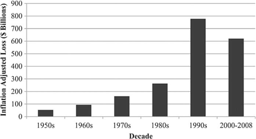
Worldwide economic loss by decade (Kunreuther et al. 2009).

There are many questions that arise in mitigation planning and response that require an estimate of the impact of a single earthquake scenario on a region. This event might be the repetition of a historical event of significance like the 1812 New Madrid earthquake, or an event developed from a seismic study, similar to the ShakeOut scenario developed for Southern California in 2008 (USC 2008).

Over the last 20 years, significant progress has been made in the construction of loss estimation methodology. As an illustration of that success, HAZUS is a loss estimation methodology developed by FEMA (2010) that serves as the standard in the estimation of damage to buildings and individual elements of transportation and utility systems based on a single event. The key idea which underlies earthquake loss estimation methodologies is the integration of two pieces of data for each element in the built infrastructure. The first element is a vulnerability model that is dependent on the type of structure, and the second element is a probability distribution for the ground shaking at that location based on the event. A vulnerability model specifies the probability that a structure of a specific type experiences a certain level of damage or greater for a given amount of ground shaking. The second element is a probability distribution for the ground shaking at the location of interest. This ground shaking is estimated using ground motion prediction equations, which predict the distribution of ground motion amplitudes often assuming a logarithmic mean that represents the distance, magnitude, type of rupture, soil classification, etc., and a standard deviation. It is commonly assumed that the residuals, as estimated by the standard deviation, are normally distributed about the mean. Many ground motion prediction equations also include a component to address the correlation that exist in ground shaking at different locations beyond that simply associated with soil classification, and the distance between the source and each site (e.g., Bommer and Crowley 2006, Lee and Kiremidjian 2007).

The result of bringing together these two types of information is an estimate of the probability, for each component in the study area that the component will be in one of several mutually exclusive and exhaustive damage states. For example, for a specific highway bridge there might be a 50%, 30%, 10%, 6%, and 4% chance that it will be in no damage, slight damage, moderate damage, extensive damage, and complete damage, respectively. Notice, this does not say which damage state the bridge will be in, only the probability that it will be in each state. Further, the performance of a highway system is driven by the damage to all the bridges because each bridge affects the connectivity of the network. Therefore, in order to assess the functionality of a lifeline system it is not only important to understand what might occur to each of the components but it is also important to understand the joint distribution of damage to all components since system functionality depends on how all components perform together. Hence, we define the term consequence scenario. For our purposes, a consequence scenario gives the damage state experienced by each system component after the event. A suite of these scenarios will be needed to assess the impact of an event.

The common strategy used to construct consequence scenarios is Monte Carlo sampling, which requires a large number of samples. Since performing computationally intensive calculations on a large number of samples is impractical, in practice small sample sizes are used or the computations performed on each sample observation are simplified. Chang et al. (2000) randomly generates ten consequence scenarios for each single event using the probabilistic information derived for each bridge to analyze the impacts of earthquakes on the Los Angeles highway system. Shiraki et al. (2007) extend the analysis in Chang et al. (2000) to consider 47 earthquake events using 10 Monte Carlo sample realizations of each event. Our analysis can be viewed as a complementary analysis in which we apply optimization to generate the realizations of each event in lieu of Monte Carlo simulation. Çağnan et al. (2006) use a mixture of Monte Carlo simulation and expert opinion to model the Los Angeles electrical system with 10 or 20 Monte Carlo samples to assess the impacts of an event. Jayaram and Baker (2010) apply Monte Carlo sampling to the San Francisco highway system. They show that about 150 ground motion intensity maps are needed to represent the hazard. For each ground motion map they use simulation to assess system performance using fragility curves. A novel element of their analysis is the use of data reduction techniques to reduce the number of ground motion maps. As in Shiraki et al. (2007), this analysis can also be viewed as complementary to that given in Jayaram and Baker (2010) in that we propose a method to generate damage maps using optimization instead of Monte Carlo simulation of ground motion maps.

This paper describes an alternative method to identify a set of consequences that can be used in regional loss estimation in lifeline systems when computational demands are of concern, and the spatial coherence of individual consequence scenarios is important. It extends Brown et al. (2011) by including correlation in the damage model. Computation may be of particular concern: (1) when there are computationally intensive analyses to be conducted for each consequence scenario, as when one estimates damage to a lifeline network for each consequence scenario, then estimates service restoration times for each consequence scenario (e.g., Xu et al. 2007), or (2) when loss estimation must be repeated many times, as when evaluating the relative benefits of many mitigation alternatives (e.g., Dodo et al. 2005).

The following section describes an optimization model and an associated solution procedure that can be used to identify a set of consequence scenarios and a probability for each scenario. The third section describes a realistic case study. The fourth section presents conclusions and opportunities for future research. For ease of presentation, we describe this model in the context of a transportation network and illustrate its application to a road network in Memphis, Tennessee, but it could be applied to any spatially distributed lifeline systems by replacing the notion of a bridge by the relevant components (e.g., substations, switching centers).

Optimization Model

The goal of the optimization model is to create a set of consequence scenarios that, in combination, approximate the vulnerability of each component of an infrastructure under a specific earthquake event and the correlation in that vulnerability across components. The key inputs to the model are the marginal damage distribution of each component of an infrastructure for the earthquake event as well as the covariance in that damage. The marginal distribution is the probability that a component is in each of a set of mutually exclusive and exhaustive damage states and is defined by a loss estimation methodology, such as HAZUS. This distribution represents the vulnerability of the component. Additionally, the user specifies the desired number of consequence scenarios. The output of the optimization model is a collection of consequence scenarios. Each consequence scenario has a realized damage state for each component of the infrastructure and an associated probability. For a given component, the damage state and probability from each scenario can be used to determine the implied vulnerability. Also, these implied vulnerabilities can be used to determine the correlation in damage across components. The objective of the optimization is to select the consequence scenarios and associated probabilities so that the implied vulnerabilities of each component and the covariance in those vulnerabilities match the “true” (input) conditions as closely as possible.

Figure 2 illustrates the core idea of the model for a single component and the marginal distribution of damage i. The diamonds represent the “true” vulnerability given by the marginal damage distribution. For the purposes of the case study, the marginal damage distribution is the result of applying the ground motion prediction equations at that location and using the fragility curves to compute the probability that the bridge falls into each damage state. The squares represent the vulnerability implied by aggregating (by their probability of occurrence) the consequence scenarios generated by the model for that bridge, for each damage state. The goal is to minimize the squared difference between the “true” and implied vulnerabilities. That difference is illustrated by the value of the variable e_kd, which is defined as the difference in the “true” and implied vulnerabilities for bridge k and damage state d. We choose to minimize the squared errors under the assumption that it is preferable to have relatively more deviations with small magnitudes than a smaller number of large deviations.

Figure 2.

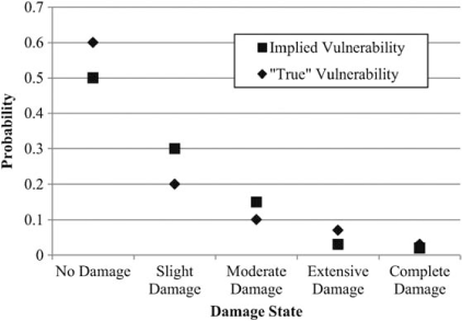
Schematic defining the error terms between the “true” vulnerability of the bridge under the specific event and the vulnerability represented by the set of consequence scenarios (and their probabilities) generated by the model.

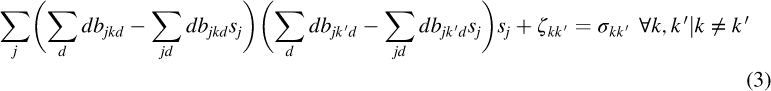
We formulate the optimization as a nonlinear mixed integer problem. The two key decision variables are s_j, which is the hazard-consistent annual occurrence probability of consequence scenario j, where J is the number of consequence scenarios to be generated, and b_jkd is a binary variable that is 1 if bridge k falls into damage state d under consequence scenario j, and 0 otherwise. We assume that the probability that bridge k falls into damage state d as estimated by the loss model is given by m_kd, where d ∈ (1, …, D). The first set of constraints defines the error terms for each bridge and damage state, as the difference between the probability that bridge k falls into damage state d as estimated by the loss estimation methodology, and that probability as estimated by the consequence scenarios and their likelihoods of occurrence:

\sum_{j} s_{j} b_{j k d} + e_{k d} = m_{k d}, \forall k, d

(1)

where e_kd is the error resulting from overestimating/underestimating the probability that bridge, k, falls into damage state, d. The error e_kd is negative if the value implied by the consequence scenarios is greater than the “true” value; conversely, e_kd is positive if the value implied by the consequence scenarios is less than the “true” value. It is useful to notice that if matching the values for some bridges is more important than for others, a bridge-specific weight can be added to the objective function. For example, it might be more important to match the marginal distributions on bridges that experience relatively higher traffic levels.

It is important to observe that the left-most term is nonlinear, as it contains terms that are the product of the probability of a consequence scenario and the assigned damage state under the consequence scenario. s_j can be considered a weight rather than a probability because it cannot be argued that all possible consequence scenarios are identified, and a probability is computed for each. We choose to use the term probability instead of weight because the right-hand side of Equation 1 is a true probability.

The collection of damage scenarios identified should match the spatial correlation in damage that stems from the ground motion, that is, that which stems from intra-event correlation, as well as similarities in the design, contractors, etc. between bridges (Lee and Kiremidjian 2007 and Bazzurro and Luco 2005). In practice, our ability to understand and capture the spatial correlation from the ground motion is more advanced than from other sources (e.g., common contractors, etc.). We extend the formulation above to allow the explicit inclusion of this correlation, regardless of the source.

Given that b_jkd is a binary variable that is 1 if bridge k falls into damage state d under consequence scenario j and 0 otherwise, the expected condition of bridge k under scenario j is defined by ∑_ddb_jkd. Therefore, the expected damage state of bridge k considering all the scenarios is given by ∑_jddb_jkds_j. The difference between the condition of bridge k under scenario j and the expected condition of bridge k over the set of scenarios is ∑_ddb_jkd – ∑_jddb_jkds_j. From the definition of covariance, the covariance of two bridges k, k ^′ over the set of scenarios is as given in Equation 2 below.

\sum_{j} (\sum_{d} d b_{j k d} - \sum_{j d} d b_{j k d} s_{j}) (\sum_{d} d b_{j k^{'} d} - \sum_{j d} d b_{j k^{'} d} s_{j}) s_{j} \forall k, k^{'} | k \neq k^{'}

(2)

Let σ_kk^′ be the covariance in the damage between pairs of bridges. The following constraint is then used to minimize the difference between the covariance based on the set of the scenarios and the “true” covariance:

\sum_{j} (\sum_{d} d b_{j k d} - \sum_{j d} d b_{j k d} s_{j}) (\sum_{d} d b_{j k^{'} d} - \sum_{j d} d b_{j k^{'} d} s_{j}) s_{j} + ς_{k k^{'}} = σ_{k k^{'}} \forall k, k^{'} | k \neq k^{'}

(3)

where ς_kk ^′ is the errors resulting from overestimating/underestimating the “true” covariance between bridge k and k^′.

Under each consequence scenario j, each bridge k must be in exactly one damage state d. The following constraint ensures this:

\sum_{d} b_{j k d} = 1 \forall k, j .

(4)

The probability of each consequence scenario j, must be between user-specified values s_min and s_max, where 0 ≤ s_min < s_max ≤ 1, as given in Equation 5:

s_{\min} \leq s_{j} \leq s_{\max} \forall j

(5)

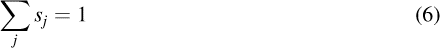
One would typically assume that s_min and s_max are 0 and 1, respectively, but if desired, the user can specify s_min > 0 and s_max < 1. It may be awkward to explain very small, as well as very large, values for s_j, and this provides a mechanism to prevent that situation. Also, the sum of the probabilities across all consequence scenarios must equal 1. The constraint that enforces this requirement is given in Equation 6:

\sum_{j} s_{j} = 1

(6)

It is worth noticing that Equations 5 and 6 are not strictly necessary. If we consider that the values s_j are in fact weights, there is no need for their sum to equal 1 or to bound the values of the weights. However, constraining these values aids in communicating the results of the optimization to others and, more importantly, in the interpretation and in the covariance calculation given in Equation 3. Finally, the error terms are unrestricted in sign. Further each bridge, under each consequence scenario, must be in a single damage state:

e_{k d} unrestricted \forall k, d

(7)

ς_{k k^{'}} unrestricted \forall k, k^{'}

(8)

b_{j k d} \in {0, 1} \forall j, k, d

(9)

The objective function is to minimize the discrepancies that stem from Equations 1 and 3 as given in Equation 10 below where α is the relative importance of minimizing the errors in the resultant spatial correlation to the errors in the resultant marginal distributions of damage.

\min \sum_{k d} e_{k d}^{2} + α \sum_{k, k^{'}} ς_{k k^{'}}^{2}

(10)

The optimization model is a nonlinear integer program where the objective is given in Equation 10 and the constraints in Equations 1 and 3 through 9. The model output is a set of consequence scenarios along with the probability of each consequence scenario j, s_j, as well as the damage state for each bridge under that scenario, b_jkd. It also provides the errors, e_kd for each bridge and damage state and the errors in the covariance between pairs of bridges, ς_kk^′.

This model is challenging to solve because it is both nonlinear and integer. It is worth noticing however that if the variables b_jkd are known the resultant optimization is nonlinear (but not integer). We use the active set algorithm in the MATLAB library to solve this reduced optimization problem (for information on the active set algorithm, see Nocedal and Wright 2006). The key idea underlying the method is to use iterations to conclude which constraints are binding at optimality (and therefore which constraints constitute the active set). The iterations use information on the Lagrangian multipliers for the constraints and infeasibilities between the constraints in the set and outside the set to update the members of the set.

If we assume that the values of the variables s_j are known, the resultant optimization is still nonlinear and integer but the evaluation of a solution of that optimization is very inexpensive. We use a local search algorithm to solve for the variables b_jkd when the variables s_j are known. We define a neighboring solution to an existing solution as one for which all variables b_jkd are the same except two and those two are the result of moving a single bridge from one damage state to another under a single consequence scenario. Given this definition for a neighboring solution, all that is necessary to compute the value of neighboring solution is the computation of the errors in the marginal distribution for the single bridge under this swap and the covariance of this single bridge with all other bridges (not all bridges with all other bridges). The algorithm stops when there are no moves of this nature that improve the objective function. Notice that there is no guarantee that this algorithm will produce the optimal solution.

The solution procedure is then as follows:

Assume that the values of all the variables s_j are 1/J and solve the resultant nonlinear mixed-integer program for the variables b_jkd for each bridge using the local search algorithm where initially bridges are simply randomly assigned to damage states under each scenario.

Fix the values for b_jkd using the solution identified in Step 1 and solve the resultant nonlinear program for the variables s_j using MATLAB.

Fix the variables s_j and again solve the mixed-integer nonlinear program for the variables b_jkd for each bridge using the local search heuristic described above.

Iterate between Steps 2 and 3 (where Step 2 is executed using the values for the variables b_jkd identified in Step 3) until no improved solution is found.

It is worth noting that at each iteration of the algorithm, the objective function value given in Equation 5 will either improve or remain the same. It is this observation that leads to the simple stopping criteria given in Step 4 of the algorithm.

Finally, this solution procedure begins by assuming that each consequence scenario is equally likely, and a random start for the variables, b_jkd, is used. Therefore, depending on the values drawn for the variables, b_jkd, a different solution may be identified at convergence. Hence it is useful to apply this algorithm several times, each with different initial solutions and simply use the best solution identified.

Case Study

This section presents a case study application of the model to assess the vulnerability of the highway network in Memphis, Tennessee, to an event with a moment magnitude of 7.7 and epicenter at the Mississippi River halfway between Mississippi and Kentucky. Memphis is located in the southwest corner of the New Madrid Seismic Zone (NMSZ), as illustrated in Figure 3.

Figure 3.

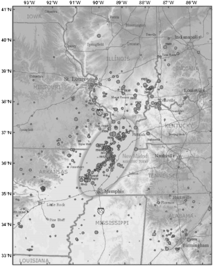
New Madrid Seismic Zone. Dots are historical earthquakes. Polygons are metropolitan areas (Frankel et al. 2009).

Figure 4 provides some insight into the level of congestion in the Memphis road network using the Travel Time Index and the Roadway Congestion Index for 101 cities considered in the Texas Transportation Institutes Annual Mobility Report released in 2010. The Travel Time Index is a measure of the increase in travel time experienced during the peak in contrast to when free flow speeds are available. The natural range of this statistic is one and above, with smaller numbers indicating less congestion. The Roadway Congestion Index is an approximate measure of the density of traffic across the urban area. The natural range of this statistic is 0 and larger with smaller values indicating lower levels of congestion. Notice that some cities have values that exceed one indicating “high” levels of congestion. For the Memphis urban area, the Travel Time Index is about 1.13 and the Roadway Congestion Index is 0.86. This area has far more desirable values than those for cities like Los Angeles, California, and Washington, D.C. Based on the Travel Time Index and the Roadway Congestion Index, Memphis ranks 44st and 67th (out of 101 cities), respectively.

Figure 4.

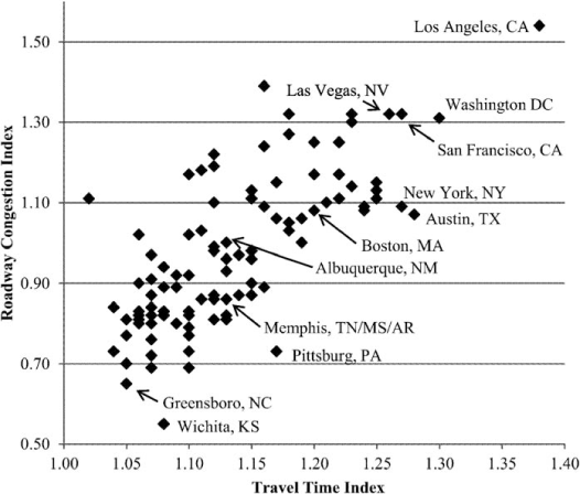
Travel time index and roadway index for select U.S. cities (TTI 2010).

Input Data and Route Choice Behavioral Assumption

As mentioned previously, this case study focuses on an event with a moment magnitude of 7.7 and epicenter at the Mississippi River halfway between Mississippi and Kentucky. This location is on the Mid-East branch of the synthetic faults created by the U.S. Geological Survey (USGS) to represent part of the earthquake hazard in the New Madrid Seismic Zone (Peterson et al. 2008).

For this study, we focus on developing consequence scenarios to estimate the performance of the Memphis road network under this event. The key vulnerabilities considered are to the 335 highway bridges in Shelby County, built prior to 2000, based on the National Bridge Database included in HAZUS. Figure 5 illustrates this highway network.

Figure 5.

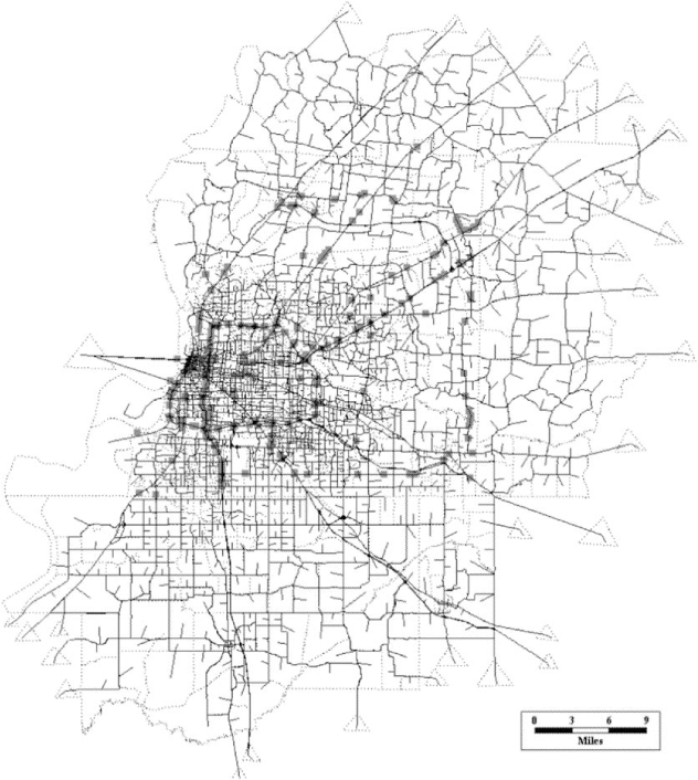
Memphis highway network, traffic analysis zones and bridges (squares).

The spectral accelerations (0.3 s and 1 s) produced by this event at each of the bridges are computed using the procedure described in Peterson et al. (2008) using code provided by USGS (2008). This procedure did not include parameters for the representation of intra-event correlation hence we assume that there is no covariance in the ground shaking when we populate Equation 4. More specifically, this implies that the covariance in the bridge damage between pairs of different bridges is assumed to be 0. We use the five damage states for each bridge as given in HAZUS: no damage, slight damage, moderate damage, extensive damage, and complete damage and compute the probability that each bridge is in each of the five damage states using the procedure given in FEMA (2010).

We use the difference in the estimated travel time distribution based on peak-period trips (trips between 6:00 a.m. and 9:00 a.m. for a total of about 560,000 trips) pre- and post-event as a measure of the seismic vulnerability of the road infrastructure to this event. We assume that the underlying origin-destination table is the same both pre- and post-event. While traffic demand is likely to change after the event, it is not clear how it would be altered, and estimating this alteration would cloud our understanding of the change in the capabilities of the road network stemming from the event. We estimate the pre- and post-event travel time distributions using the principle of dynamic user equilibrium (DUE). The underlying behavioral assumption behind DUE is that each individual traveler dynamically chooses a route that minimizes their travel time to the destination. That is, as travel conditions change on the network, drivers adapt so as to minimize their travel time. DUE is a generalization of user equilibrium (UE), which is a static analysis that simply assumes that each traveler selects a fixed path that minimizes their travel time. The generalization of UE to DUE allows for a more accurate representation of the traffic dynamics as they unfold over time. However, it also requires the development of an origin-destination table for each time period during the planning horizon. We use 15-minute time periods over a three-hour time span to represent travel during the peak period. The algorithm employed is discussed at length in Li et al. (2011). The translation of the origin-destination table for the peak period into a series of origin-destination tables (one for each period) is done based on data in the Memphis Metropolitan Planning Organization Long-Range Plan (2011).

Model Results and Discussion

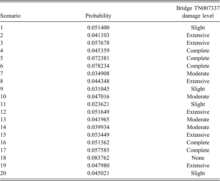
As discussed in the “Optimization Model” section above, the output of the optimization model gives a set of consequence scenarios for which the damage state for each bridge under each consequence scenario is identified. It also gives the probability of each consequence scenario. Table 1 gives the probability of each consequence scenario when the optimization model was used to develop 20 consequence scenarios and their probabilities. For example, the probability of the first of the 20 scenarios is 5.14%. Figure 6 illustrates the damage state for each bridge under that consequence scenario (Scenario 1). As a further illustration of the model outputs, Table 1 also gives the damage state under each consequence scenario for a bridge on State Route 51 near Millington (with HAZUS bridge classification HWB5 and ID TN007337), also identified in Figure 6, as an illustration of the variables b_jkd in the model. Table 2 illustrates how the implied vulnerability is determined from the results in Table 1 for bridge TN007337. The implied vulnerability column shows the resulting marginal damage distribution based on the 20 consequence scenarios and their probability of occurrence. The value of the implied vulnerability for no damage is determined by adding the scenario probabilities of all scenarios where the bridge was in the no damage state (Scenarios 3 and 8), the remaining implied vulnerabilities are determined in the same fashion. We provide a large number of significant digits in Tables 1 and 2 to illustrate the computations of the implied vulnerability and the error values only. In practice, these values would be rounded appropriately. It is important to remember that in the objective, the sum of the square of the errors is used. For this bridge and this suite of consequence scenarios, that sum is 0.000396.

Figure 6.

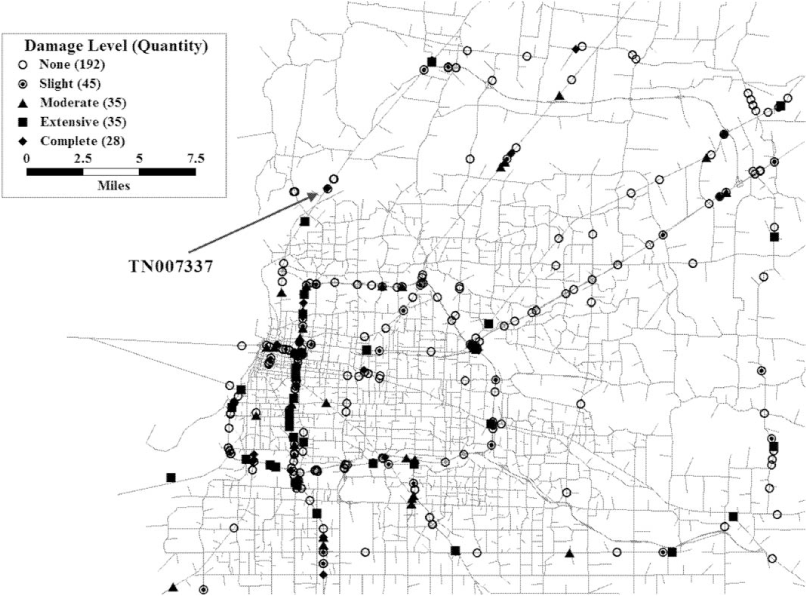
Damage state for each bridge under Consequence Scenario 1.

Table 1

Consequence scenario probabilities from optimization for 20 scenarios

Scenario	Probability	Bridge TN007337 damage level
1	0.051400	Slight
2	0.041103	Extensive
3	0.057678	Extensive
4	0.045359	Complete
5	0.072381	Complete
6	0.078234	Complete
7	0.034908	Moderate
8	0.044348	Extensive
9	0.031045	Slight
10	0.047016	Moderate
11	0.023621	Slight
12	0.051649	Extensive
13	0.041965	Moderate
14	0.039934	Moderate
15	0.053449	Extensive
16	0.051562	Complete
17	0.057585	Complete
18	0.083762	None
19	0.047980	Extensive
20	0.045021	Slight

Table 2

Comparison of the “true” vulnerability and implied vulnerability for bridge TN007337

Damage level	“True” vulnerability	Implied vulnerability	Absolute error
None	0.105679	0.083762	0.004864
Slight	0.147006	0.151870	0.014143
Moderate	0.149689	0.163832	0.010938
Extensive	0.285269	0.296207	0.007237
Complete	0.312358	0.305121	0.004864

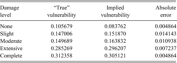
Figure 7 gives a histogram of the covariances between bridge TN007337 and all other bridges using the 20 consequence scenarios for which the probabilities are given in Table 1. In this example, the assumption is that these covariances are assumed to be 0. It is useful to notice that the distribution of the covariance is roughly symmetric, with relatively more being of smaller magnitude. The variance in the damage for this single bridge is 1.6572, and that variance is replicated, virtually without error, using these 20 consequence scenarios.

Figure 7.

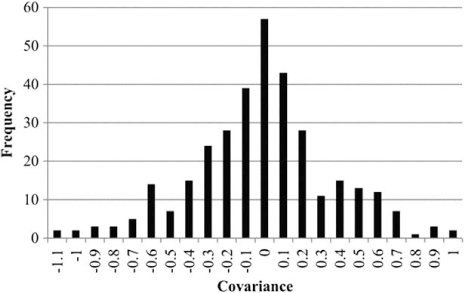
Histogram of the covariance in damage between bridge TN007337 and all other bridges.

The optimization model was solved for 10, 20, and 40 consequence scenarios (with five different values for the weight α in the objective function), and for comparison, a Monte Carlo simulation was performed to generate 20, 50, 100, 200, and 500 consequence scenarios. Figure 8 gives the trade-off frontier between the sum of the absolute value of the covariances (which includes the sum of the variances) and the sum of the absolute value in the errors in the marginal damage distributions. In this example, ideally, the covariance in the damage between pairs of bridges should be 0 across the consequence scenarios. The sum of the variances in the bridge damage should be about 444 (∑_kσ_kk² = 444). Again, it is important to remember that the optimization is performed by minimizing the square of the errors; however, the trade-off frontiers are given based on the sum of the absolute value in the errors and the sum of the covariances because it is easier to understand these values.

Figure 8.

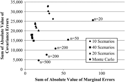
Trade-off frontier.

The range in the sum of the absolute value of the errors in the marginal distribution for ten consequence scenarios is from about 29 to 36. Using Monte Carlo simulation, about 100 scenarios are needed to reach this level of precision. However, the sum of the covariances is about 11,000 using the 100 Monte Carlo simulations, whereas it about three times that amount for the 10 scenarios developed using optimization. Remember, the goal is to have this sum be 444 (only the variances should be non-zero).

Figure 9 gives box plots to indicate the estimated distribution of computation time (per random start) by number of scenarios. All experiments were performed on a 2.67 GHz PC with 12 GB of memory. Since there are five weights considered for 10, 20, and 40 scenarios, and for each combination, 10 replicates are performed (since this algorithm begins with random values for the b_jkd variables); there are 50 experiments for each number of consequence scenarios. It is useful to notice that the variation in the computation time does increase substantially when 40 consequence scenarios are developed, most of which is attributable to the MATLAB nonlinear solver.

Figure 9.

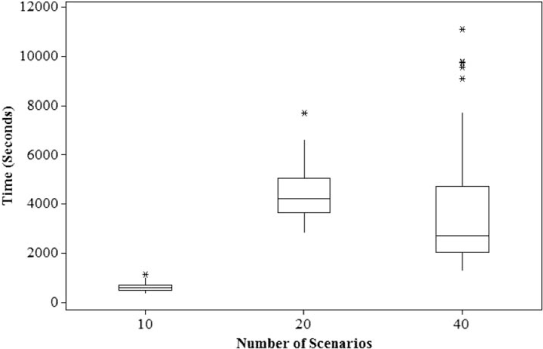
Estimated distribution for computation time by number of consequence scenarios requested (median, 90th and 10th percentile).

Estimating Impacts on Traffic

The goal of the creation of consequence scenarios is the accurate estimation of the impact of the earthquake event on traffic. Therefore, the remainder of this subsection assesses how this estimate varies based on the method used to generate the scenarios.

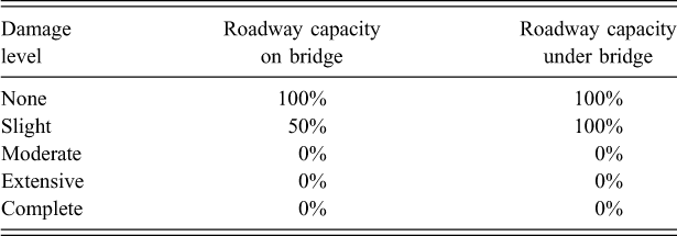
In order to do an analysis of the capabilities of the road network after an earthquake event, we need to translate the damage state for each bridge into the capacity of both the roadways on and under the bridge to accommodate traffic. HAZUS (FEMA 2010) gives restoration curves for highway bridges in each damage state that show the bridge functionality over time. For roadways on bridges, we assume that if the damage state implies a functional percentage of less than 50%, the roadway cannot be used; if a functional percentage between 50% and 75%, the roadway has 50% capacity; if a functional percentage between 75% and 95%, the roadway has 75% capacity; and full capacity otherwise. For roadways under the bridge, we assume that when the functional percentage for the bridge is below 50%, they cannot be used, and with a functional percentage over 50%, the roadway has full capacity. Since the functionality from the restoration curves depends on the number of days since the event, there will be several stages of recovery before full capacity is available on all roadways. For this analysis, we only consider the capacity impacts in the immediate aftermath of the event. Table 3 shows how these assumptions translate into roadway capacities for each bridge damage state in the immediate aftermath of the earthquake.

Table 3

Roadway capacities as a percent of their pre-event capacity for each damage state immediately after the earthquake event

Damage level	Roadway capacity on bridge	Roadway capacity under bridge
None	100%	100%
Slight	50%	100%
Moderate	0%	0%
Extensive	0%	0%
Complete	0%	0%

As mentioned previously, we use Li et al. (2011) to develop the travel time distribution, pre- and post-event. The key advantages of the DTA algorithm in Li et al. (2011), in contrast to other DTA algorithms, is the computation time. Applying this algorithm, developed in Java, to this case study when there is no bridge damage requires about 6.3 minutes using 15-minute time periods for a three-hour peak-period analysis on a PC with a 2.66 GHz Intel Xenon X5355 processor and 32 GB of RAM. The longest computation time of 12.5 minutes was experienced when all 335 bridges are unavailable. The computation time of the DTA algorithm stemming from a consequence scenario generated using optimization or via Monte Carlo simulation was between 6.3 and 10.0 minutes.

Figure 10 gives a histogram of the peak period travel time (using morning peak origin-destination tables) when all bridges are intact, after an assumed loss of all 335 bridges, under 1 of the 20 (mid-level value for α) consequence scenarios identified through the optimization and under 500 randomly generated scenarios. It is also important to remember that we only model the loss to bridges included in HAZUS because that is the source of the fragility curve information. It is useful to notice that under normal conditions (no damage), the travel times are rather short, with about 51% of the trips requiring less than 12 minutes to complete (remember, as illustrated in Figure 4, the traffic level in Memphis is light). Under complete damage, this percentage dips to about 32%. Averaged across the 20 scenarios based on the probability of each scenario, this percentage is about 44%. Averaged across the 500 randomly generated scenarios, this percentage is about 45%. Notice that the estimated travel time distribution is very similar, whether the 20 scenarios are used or the 500 randomly generated scenarios, suggesting that a small number of scenarios are, in fact adequate.

Figure 10.

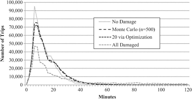
Estimated travel time distribution for trips during the peak period (6:00 a.m.–9:00 a.m.).

Figure 11 illustrates the relationship between the number of bridges on the path for a trip based on the DTA algorithm when there is no damage to the infrastructure and the average increase in travel time experienced over the 20 consequence scenarios (developed using the optimization). About 33% of trips use a route that does not traverse or pass under a bridge when there is no bridge damage. About 60% of trips traverse or pass under no more than 2 bridges (when there is no bridge damage). As a consequence, on average, there is relatively little impact on these trips under the 20 consequence scenarios developed. However, as the number of bridges needed by a trip in the no-damage scenario increases, the impact of the consequence scenarios on these trips increases.

Figure 11.

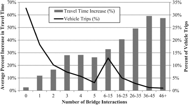
Relationship between the number of bridges traversed or passed under when there is no bridge damage and the increase in travel time experienced.

The average number of trips that cannot be completed based on the 20 scenarios is about 6,200, with a maximum of about 15,100 and a minimum of about 1,400. Based on the 500 Monte Carlo scenarios, the minimum is 0, with a maximum of about 14,100 and an average of 3,400 trips. If all bridges were to be unavailable, about 94,700 trips would not be completed.

Table 4 gives the estimated percentage of trips made during the peak period based on the number that could be completed with a travel time greater than 12, 24, 36, 48, and 60 minutes when there is no damage to any of the 335 bridges, all of the bridges are in complete damage, using the 20 scenarios developed via the optimization method, and using the 500 scenarios developed via Monte Carlo simulation. Again, this table also illustrates that in the absence of an earthquake, the travel times are rather short, with about 51% of trips requiring less than 12 minutes to complete. When considering the statistics given in Figure 10, Table 4, and the discussion regarding how many trips that can no longer be completed, it is useful to notice that the scenarios developed via optimization are very similar but slightly more pessimistic than those developed using Monte Carlo simulation. It is reasonable to conclude that the package of scenarios developed via optimization is more pessimistic because there is more correlation in the damage across bridges than in the random sample of 500. In actuality, the correlation in the damage between bridges should be 0. Five hundred samples are not sufficient to reach this ideal of 0, but it is significantly closer than with the 20 scenarios developed using optimization.

Table 4

Percent of trips in different travel time categories for different groups of scenarios. For the Monte Carlo case the sample standard deviation is given in parentheses

Scenario	≥ 12 minutes	≥ 24 minutes	≥ 36 minutes	≥ 48 minutes	≥ 60 minutes
No damage	49%	11%	1%	0%	0%
Complete damage	68%	47%	37%	33%	31%
Average for 20 scenarios	56%	20%	5%	1%	0%
Average Monte Carlo (500 scenarios)	55% (1.2%)	18% (1.3%)	4% (0.9%)	1% (0.4%)	0% (0.1%)

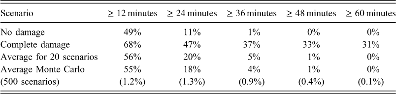
Figure 12 gives the total volume carried over the peak period for each facility when there is no earthquake damage. Much of the traffic is concentrated on Interstates I-40, I-55, and I-240. Figure 13 gives that same information but where the volumes are averaged over the 20 consequence scenarios based on their probability of occurrence. It is useful to consider Figure 13 in the context of Figure 5 also. Notice the large number of bridges that exist on I-40 and I-240. The key observation when considering Figure 13 is that Interstate I-40 south of SR-300 is effectively not available. Further, I-240 is effectively unavailable south of I-40 to approximately Getwell Road and I-55 is effectively unavailable as well. Much of the traffic is therefore diverted onto smaller facilities like Watkins Street, Covington Pike, and Airways Boulevard, for example.

Figure 12.

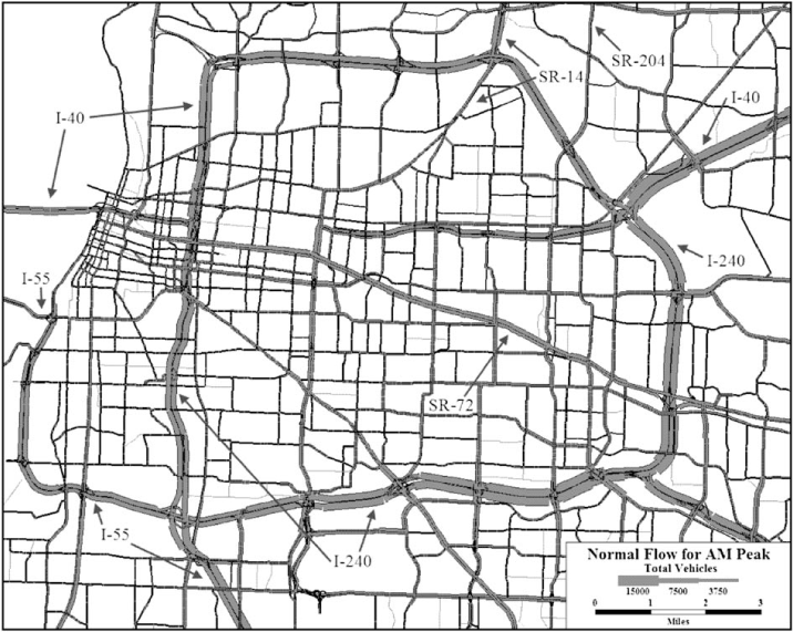
Estimated total peak period volume in the absence of earthquake damage.

Figure 13.

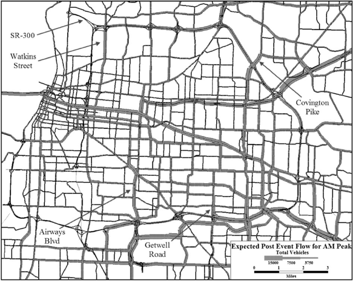
Estimated average total peak period volume based on the 20 consequence scenarios stemming from the optimization.

Conclusions

This paper presents a new optimization approach to identify consequence scenarios for estimating the impact of an earthquake event on lifeline systems. A novel nonlinear integer program is developed and used to identify a small set of damage events and the probability of occurrence for each, such that together they match the damage probabilities for each component as given in the loss estimation modeling (e.g., FEMA 2010). This set of events will allow system performance to be estimated with a high degree of accuracy while keeping the computational burden to a minimum.

There are opportunities for further research in at least two areas. The solution procedure developed relies on a solver in MATLAB to optimize the value of the consequence scenario probabilities given the scenarios themselves. Based on the experiments conducted, as the number of consequence scenarios needed rises, the variation in the solve time increases. Therefore, there is value in developing a new approach to solve this optimization problem. A global search heuristic like simulated annealing could prove to be useful in the construction this new approach. It could also be useful to integrate that type of a procedure with other techniques, such as response surfaces. Of course, the application of these approaches may have important impacts on the solution time as well as the solution quality.

Second, this case study focused on developing consequence scenarios for a single event, which is of significant value. However, if the goal is to use these scenarios to understand the seismic vulnerability of an area, it is important to extend the optimization to simultaneously identify consequence scenarios for the range of events (and the hazard-consistent probability of occurrence for each) that represent the seismic vulnerability of the area. Clearly this optimization could be run for each of the events separately, but that may make it hard to identify how many consequence scenarios should be used for each event when there is a maximum total number of scenarios that can be included in further analyses. It would also make it difficult to include inter-event correlation in the development of the scenarios.

References

Brown

N. J. K.

, Gearhart

J. L.

, Jones

D. A.

, Nozick

L. K.

, Xu

, and Romero

, 2011. Optimizing the selection of scenarios for loss estimation in transportation networks, in Proceedings of the 2011 WSC: Simulation for a Sustainable World, Phoenix, AZ.

Bazzurro

, and Luco

, 2005. Accounting for uncertainty and correlation in earthquake loss estimation, in Proceedings of the 9th International Conference on Structural Safety and Reliability, Rome.

Bommer

J. J.

, and Crowley

, 2006. The influence of ground-motion variability in earthquake loss modeling, Bulletin of Earthquake Engineering 4, 231–248.

Çağnan

, Davidson

, and Guikema

, 2006. Post-earthquake Restoration Planning for Los Angeles Electric Power, Earthquake Spectra 22, 1–20.

Chang

, Shinozuka

, and Moore

, 2000. Probabilistic earthquake scenarios: Extending risk analysis methodologies to spatially distributed systems, Earthquake Spectra 16, 557–572.

Dodo

, Xu

, Davidson

, and Nozick

, 2005. Optimizing regional earthquake mitigation investment strategies, Earthquake Spectra 21, 305–327.

Federal Emergency Management Agency (FEMA), 2010. HAZUS User and Technical Manual, Department of Homeland Security, http://www.fema.gov/plan/prevent/hazus/hz_manuals.shtm (accessed 14 March 2011).

Frankel

A. D.

, Applegate

, Tuttle

M. P.

, and Williams

R. A.

, 2009. Earthquake Hazard in the New Madrid Seismic Zone Remains a Concern, U.S. Geological Survey Fact Sheet 2009–3071.

Jayaram

, and Baker

J. W.

, 2010. Efficient sampling and data reduction techniques for probabilistic seismic lifeline risk assessment, Earthquake Engineering and Structural Dynamics 39, 1109–1131, doi: 10.1002/eqe.988.

10.

Kunreuther

, Michel-Kerjan

, Doherty

, Grace

, Klein

, and Pauly

, 2009. At War with the Weather: Managing Large-Scale Risks in a New Era of Catastrophes, MIT Press, Cambridge, MA.

11.

Lee

, and Kiremidjan

A. S.

, 2007. Uncertainty and correlation for loss assessment of spatially distributed systems, Earthquake Spectra 23, 753–770.

12.

A. C. Y.

, Nozick

, Davidson

, Brown

, Jones

D. A.

, and Wolshon

, 2012. An approximate solution procedure for dynamic traffic assignment, Transportation Engineering, in press.

13.

Memphis Metropolitan Planning Organization, 2011. Long-Range Transportation Plan (LRTP), available at http://memphismpo.org/index.php?option=com_content&view=article&id=66&Itemid=53 (last accessed January 2011).

14.

Nocedal

, and Wright

S. J.

, 2006. Numerical Optimization, 2nd Edition, Springer, New York, 664 pp.

15.

Petersen

M. D.

, Frankel

, Harmsen

, Mueller

, Haller

, Wheeler

, Wesson

, Zeng

, Boyd

, Perkins

, Luco

, Field

, Wills

, and Rukstales

, 2008. Documentation for the 2008 Update of the United States National Seismic Hazard Maps, U.S. Geological Survey Open-File Report 2008–1128.

16.

Shiraki

, Shinozuka

, Moore

J. E.

, Chang

S. E.

, Kameda

, and Tanaka

, 2007. System risk curves: Probabilistic performance scenarios for highway networks subject to earthquake damage, Journal of Infrastructures Systems 13, 43–54.

17.

State of California Department of Conservation, 2011. Northridge Earthquake 10 Year Anniversary, available at http://www.consrv.ca.gov/cgs/geologic_hazards/earthquakes/Pages/northridge.aspx (last accessed 25 February 2011).

18.

Sun-Sentinel, 2011. Ten Years After Hurricane Andrew, Effects are Still Felt, available at http://www.sun-sentinel.com/sfl-1992-ap-mainstory,0,7290462.story (accessed 25 February 2011).

19.

Texas Transportation Institute (TTI), 2010. Annual Urban Mobility Report, available at http://mobility.tamu.edu/ums/ (last accessed 16 June 2011).

20.

USA Today, 2005. Katrina Damage Estimate Hits $125B, available at http://www.usatoday.com/money/economy/2005-09-09-katrina-damage_x.htm (last accessed 25 February 2011).

21.

University of Southern California (USC), 2008. The Great California ShakeOut, available at http://www.shakeout.org/2008/ (last accessed 1 March 2011).

22.

United States Geological Survey (USGS), 2008. 2008 NSHM Software, available at http://earthquake.usgs.gov/hazards/products/conterminous/2008/software/ (last accessed June 2010).

23.

, Guikema

, Davidson

, Nozick

, Çağnan

, and Vaziri

, 2007. Optimizing scheduling of post-earthquake electric power restoration tasks, Earthquake Engineering and Structural Dynamics 36, 265–284.