





Abstract
The Mw 8.4 23 June 2001 Southern Peru earthquake generated intense ground motions in a large region encompassing southern Peru and northern Chile. The earthquake was recorded by seven strong motion stations with peak ground accelerations ranging from 0.04 g to 0.34 g for site-to-fault distances ranging from about 70 km to 220 km. At this time, there are no other strong motion records for an earthquake of this magnitude. Hence, the strong motion data set from this earthquake is unique and of particular interest to engineers dealing with seismic design in subduction regions. This paper presents an engineering analysis of the strong motion records. Shear-wave velocity profiles were measured using Spectral Analysis of Surface Waves methods at four stations. Measured shear-wave velocities are high, indicating that all sites classify as stiff soil sites (Site C) according to the International Building Code classification scheme. The strong motion set is characterized by strong high frequency content at large distances from the fault. Site response contributed at least in part to the observed high frequency content in the ground motions. In general, current attenuation relationships for spectral acceleration underpredicted the observed ground motions.
Introduction
The 23 June 2001 Southern Peru earthquake (moment magnitude, Mw =8.4) generated intense ground motions in a large region encompassing southern Peru and northern Chile (Figure 1). Medvedev-Sponheuer-Karnik (MSK) intensities (similar to Modified Mercalli Intensity values, Kramer 1996) reported by Tavera et al. (2006) were as high as VII in the coastal region bordering the ruptured fault. The earthquake was felt as far inland as La Paz, Bolivia, with an MSK intensity of III. The earthquake resulted from thrust faulting as the Nazca plate subducts beneath the South American plate. At the time it occurred, the Southern Peru earthquake was the largest seismic event in terms of energy release since 1965 (Harvard CMT 2008). It remains the largest earthquake to date to have been recorded by a strong motion seismograph network, yielding seven three-component free-field accelerographs measured within 250 km of the causative fault.
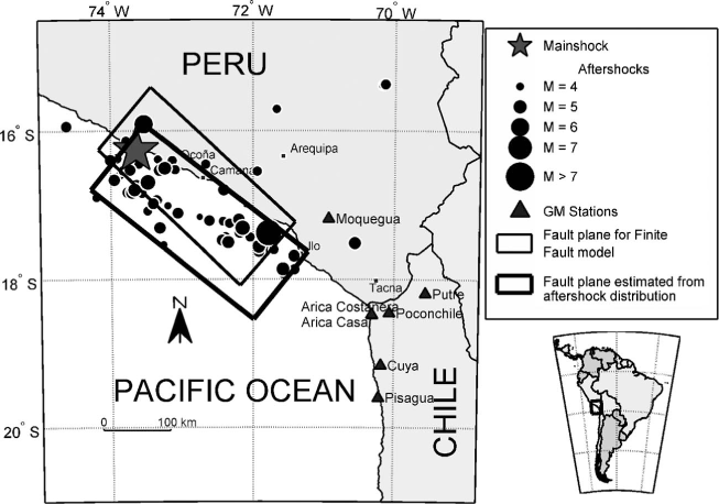
Map of the affected region showing the main shock epicenter as well as location of several aftershocks and the location of ground motion stations. Aftershock locations are obtained from the U. S. Geological Survey.
Seismic design of engineered structures often calls for the use of time-history analysis using ground motions obtained from events similar to the design event and recorded in similar tectonic and geologic environments. However, prior to the 2001 earthquake there were no strong motion records for earthquakes larger than Mw 8.3. The scarcity of strong ground motion records for megathrust earthquakes makes the recordings from this earthquake unique and of particular interest to engineers dealing with seismic design in subduction regions. This paper presents an engineering analysis of the ground motions recorded in the Southern Peru Earthquake and discusses their relevance for seismic hazard analyses in subduction zones. Ground motion parameters obtained from the recorded motions are evaluated and compared with current predictive equations.
The ground motions records were obtained on very stiff soil profiles which raises questions regarding the effect of site amplification on the recorded motions. The site conditions at four of the seven ground motion station sites have been investigated by means of spectral analysis of surface waves (SASW) field tests. The shear-wave velocity (Vs) profiles obtained from the field tests are used to estimate the contribution of site amplification from the shallow soil layers to the recorded ground motion. Despite the fact that Vs profiles at the ground motion station sites correspond to very stiff soils, site amplification appears to have affected the recorded motions.
Damage Overview and Seismotectonic Setting
A total of 149 people were killed or went missing and are presumed dead as a result of the 23 June earthquake, its aftershock sequence, and a localized tsunami generated by the main shock (INDECI 2005). The earthquake affected the major city of Arequipa, Peru, and several large population centers including Camaná, Moquegua, Ilo, and Tacna, in Peru, and Arica in Chile. Structural damage occurred primarily to adobe houses and historical buildings; however, a significant number of engineered structures also suffered damage.
Ground failure was prevalent throughout a wide area (~ 45,000 m2) and had a marked impact on the region's transportation infrastructure. Landslides in highway cuts and seismic compression (i.e., shaking-induced densification of soil) in embankments were common. Liquefaction occurred over a large area but was constrained to river valleys because of the aridity of the region. A comprehensive summary of the structural, geotechnical, and societal impacts of the earthquake is presented in Rodriguez-Marek and Edwards (2003).
The earthquake hypocenter was located off the Pacific coast (16.26°S, 73.64°W) at a depth of 30 km (USGS 2008). The reported magnitude of the earthquake varies from Mw 8.4 in the Harvard CMT catalog to Mw 8.2 as computed by Tavera et al. (2006), Kikuchi and Yamanaka (2001), and Giovanni et al. (2002). The seismotectonic setting of the region is dominated by the convergence of the Nazca and South American plates. This subduction zone has generated several large and destructive earthquakes over the last century. The 2001 earthquake occurred in a portion of a previously identified seismic gap (e.g., Dorbath et al. 1990). At the time of the earthquake sections of the subduction interface northwest and southeast of the ruptured fault remained locked and retained potential to produce large earthquakes in the region (Dewey et al. 2003). The northwest seismic gap has been associated to the 2007 Mw 8.0 Pisco Earthquake. To the southeast, a Mw 7.9 earthquake occurred on 13 June 2005, but this earthquake occurred within the subducting Nazca plate and likely did not serve as a strain release mechanism for the subduction interface. Comprehensive discussions of the seismotectonic setting of the region are presented by Giovanni et al. (2002), Dewey et al. (2003) and Tavera et al. (2006).
The 2001 earthquake was caused by thrust faulting on the interface of the Nazca and South American plates. The Harvard CMT moment tensor solution indicates a fault plane with a strike of 310°, a dip of 18°, and a rake of 63°. This fault plane matches approximately the interplate geometry (Chen et al. 2001). The rupture initiated at the northwest end of the fault plane and propagated towards the southeast. Researchers have provided differing estimates of the size of the rupture plane. For example, Kikuchi and Yamanake (2001) estimated a rupture plane of 200 km along strike by 100 km along dip using teleseismic broadband recordings from 24 stations, while Vallée (2004) estimates an along strike length of 180 km using empirical green functions. In this study the fault plane was determined from the location of M>4 aftershocks reported by the USGS up to 7 July 2001 (the date of the largest aftershock, see Figure 1). The resulting extension of the fault plane is 310 km along strike and 130 km along dip. The up-dip portion of the fault is assumed to reach the surface underneath the Pacific Ocean. A dip angle of 18° was adopted. This rupture plane agrees with that reported by Tavera et al. (2006), although the latter extends somewhat further to the south and has a larger dip angle (28°). Moreover, there is some uncertainty as to the inland extend of the rupture plane. These uncertainties may affect estimates of closest distance to the fault for some of the ground motion stations, in particular for the Moquegua ground motion station, located at less than 100 km from the fault.
Ground Motion Records
The Southern Peru earthquake was recorded by seven strong motion stations located within 250 km of the fault plane, with measured peak ground acceleration (PGA) values ranging from 0.34 g to 0.04 g (Table 1). Only one of the recording stations was located in Peru, with the remaining six stations situated in neighboring Chile. It is noted that an additional instrument was triggered in nearby Tacna, Peru; however, the full ground motion was not recorded due to an equipment malfunction.
Ground motion stations that recorded the 2001 Southern Peru Earthquake
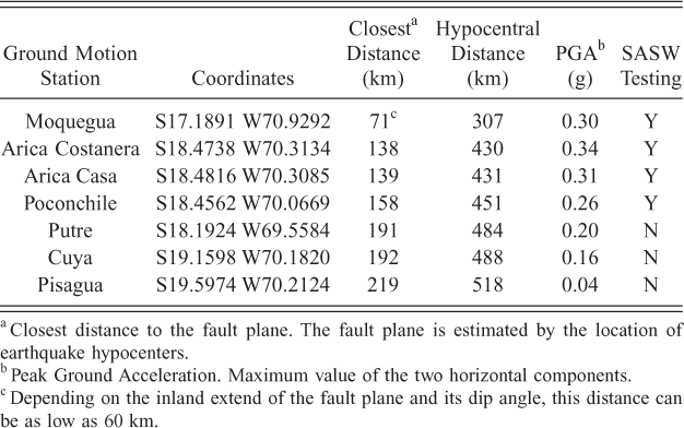
Closest distance to the fault plane. The fault plane is estimated by the location of earthquake hypocenters.
Peak Ground Acceleration. Maximum value of the two horizontal components.
Depending on the inland extend of the fault plane and its dip angle, this distance can be as low as 60 km.
The Moquegua station is owned and operated by the Peru–Japan Center for Seismic Investigation (CISMID). The instrument is located on flat ground towards the southern end of an East–West trending valley carved by the Moquegua River. The nearest topographic feature is a gently sloping hill about 100 m from the instrument. The accelerograph is housed in a wood structure located next to a one-story reinforced concrete frame building. A brick wall behind the instrument shelter apparently collapsed during the earthquake. Based on the wall height, it is not believed that the resulting impact had any significant effect on the recorded ground motions. The instrument that recorded the Moquegua record is a Rion SM-10B analog accelerograph. The record was processed by first digitalizing and then baseline correcting and filtering the data with a trapezoidal bandpass filter with corner frequencies of 0.1 Hz and 20 Hz and pass-band frequencies of 0.05 Hz and 50 Hz. Ground motion digitalization and processing is described in Aguilar and Piedra (2001). The ground motion record is available online at the CISMID Web site (http://www.cismid-uni.org/).
The Chilean records are part of the National Accelerograph Network (RENADIC) at the Universidad de Chile. The accelerographs are Kinemetrics SMA-1 instruments. Ground motion processing is described in Boroschek et al. (2001) and is similar to that used by California Strong Motion Instrumentation Program to generate Volume 2 files (Shakal et al. 2004). The Chilean records were processed by band-pass filtering with corner frequencies in the range of 0.15–0.25 Hz and 23–25 Hz. Two stations are located in the city of Arica. Arica Costanera is located along a beach-side boulevard underlain by marine and alluvial soils derived from the San Jose River. Arica Casa is located on a one story brick building situated on an elevated terrace deposit consisting of aeolic and alluvial soils. The two Arica stations along with the Putre station are located in regular topography. The Poconchile station is placed on a smooth slope in a highly arid region located approximately 25 km inland of the city of Arica. An adobe church located next to the instrument station is known to have collapsed during the earthquake, though there is no obvious evidence of this in the accelograph recording. The instrument at Cuya is located near a valley edge and is underlain by an unknown depth of soil. The instrument at Pisagua is located on a flat, rocky area near a slope and is though to be underlain by weathered bedrock. Table 1 lists the ground motion stations along with the hypocentral distance and estimated closest distance to the fault plane (Dfault). Figure 2 shows the processed acceleration and velocity time histories.
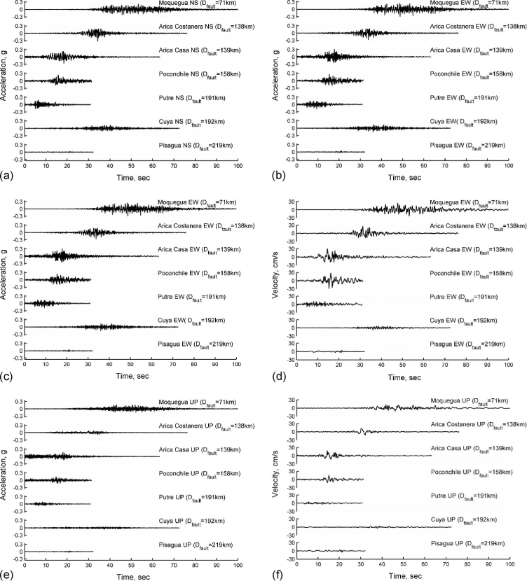
Time histories of recorded ground motions. Closest distance to the fault (Dfault) is listed for each station. (a) North–South (NS) acceleration time histories, (b) NS velocity time histories, (c) East–West (EW) acceleration time histories, (d) EW velocity time histories, (e) vertical (UP) acceleration time histories, (f) vertical velocity time histories.
Strong Motion Station Site Characterization
Site response is controlled in part by the shallow shear-wave velocity profile at the site. Spectral Analysis of Surface Wave tests (SASW) were conducted at four of the seven strong motion stations that recorded the earthquake (Table 1). As discussed later, shear-wave velocity (Vs) profiles at these sites were developed from the measured dispersion curves. Twenty-one additional shear-wave velocity profiles were developed for other sites in southern Peru as part of a larger study of site effects and ground failure during the Southern Peru earthquake (Park 2004).
Soils at the ground motion stations are typical of those found along the coast of southern Peru and northern Chile. These soils are dominated by alluvial-type deposits, composed mainly of sandy gravels with a significant fraction of boulders. This well-graded composition reflects the high-energy depositional environment resulting from the sharp topographic relief between the Andes Mountains and the Pacific Ocean. The density of quaternary deposits generally varies with depositional age. Elevated terraces have dense to very dense gravels, while more recent fluvial deposits in the river margins are, in general, looser and can include finer-grained sediments, including some silts and clays (Kosaka-Masuno et al. 2001).
The SASW test is a noninvasive in-situ geophysical method for determining shear-wave velocity profiles. The SASW method is based on the analysis of Rayleigh waves and their dispersive characteristic on a layered medium. In SASW testing a dynamic source is used to generate surface waves of different wavelengths (or frequencies) that are monitored by two or more receivers at known offsets. The testing procedure itself consists of two parts; first, measuring the surface wave dispersion curve at the site, and second, evaluating the measured dispersion curve to obtain the corresponding shear-wave velocity profile of the site. Surface waves are generated by applying a dynamic vertical load to the ground surface. Changing the spacing between the receivers and using different sources enables a broad range of soil depths to be evaluated (Stokoe et al. 1994).
The soil profile is determined through an inversion method assuming idealized, one-dimensional soil profiles. Since the solution to the inversion problem is not unique, different inversion techniques have been proposed to obtain Vs profiles. In the inversion technique used in this work, the soil density profile is assumed using standard density values for gravelly soils and a first tentative Vs profile of the site is obtained and adjusted by comparing the results of numerical simulation to the dispersion curve obtained from the field test. The WinSASW (Joh 1996) program was used to perform the inversion analysis.
A Hewlett-Packard 3562A, two-channel dynamic signal analyzer was used for data acquisition and analysis. Six 4.5 Hz geophones (GeoSpace PAT 3119978) were employed as receivers. Since one 4.5 Hz geophone outputs low amplitude signals, the signals from three geophones were combined in series acting as one receiver to increase the signal quality. Every geophone has a phase shift near its resonant frequency. This can lead to difference in measured phase velocity between two receivers. Groups of geophones with closely matched phase shifts were used in this work to minimize errors in measured phase velocity (Park 2004).
Various receiver spacings were used. Typically receiver spacings of 2, 4, 10, and 16 m were used for shallow profiling, and spacings of 20, 40, 55, and 60 m were used at sites where deep profiling was needed. Different types of wave sources were employed depending on site conditions. A small hammer was used as a wave source for the 2 and 4 m spacing; a sledge hammer was used for 8 and 10 m spacings; and a 100-kg drop weight was employed for 16 and 20 m spacings. This drop weight was raised using a lightweight aluminum tripod and hoist, then it was dropped using a quick release. A bulldozer was used for spacings longer than 20 m. The bulldozer is an excellent source to generate low frequency waves required for deep profiling. The bulldozer generated surface waves by repeatedly walking back and forth about 2 m.
Testing sites were selected as close as possible to the recordings stations. At the Arica Costanera and Arica Casa stations, the SASW lines were placed in unpaved parking lots adjacent to the structures hosting the strong motion instrument. The test at the Poconchile station was conducted on a sandy hill near the building that hosts the strong motion instrument. The SASW line was located parallel to an excavated trench. At the Moquegua station the SASW line was placed in an unpaved sidewalk across a paved road from the strong motion station. The line lay parallel to a 3.5 m high brick wall. Details on the tests setup are given in Park (2004).
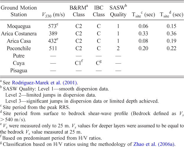
The experimental dispersion curves for the four SASW tests at the ground motion stations are shown in Figure 3. The phase plots used to generate the dispersion curve are given in Park (2004). The analytical dispersion curves obtained from forward modeling are also included in Figure 3. Due to the lack of borehole data, the values of the soil density were assumed to be 1.80 Mg/m3 for soils with Vs lower then 400 m/s, and 1.95 Mg/m3 for soils with higher shear-wave velocity. Units with Vs higher than 700 m/s were assumed to have a density of 2.1 Mg/m3. The assumed values of mass density have a small effect on the calculated shear-wave velocities. Poisson's ratio was fixed at 0.3 for all units; assumed values of Poisson's ratio also have a small effect on the calculated shear-wave velocities in unsaturated soils. The shear-wave velocity profiles obtained from the forward modeling are shown in Figure 4. The average shear-wave velocities in the top 30 m of each site (VS30) are listed in Table 2 along with corresponding site classifications using the International Building Code (IBC) system (ICC 2006) and the classification system of Rodriguez-Marek et al. (2001).
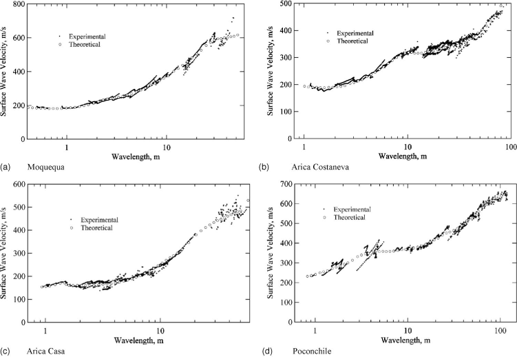
Experimental dispersion curves obtained from SASW testing along with theoretical dispersion curve from forward modeling using the selected Vs profile for each ground motion station site.
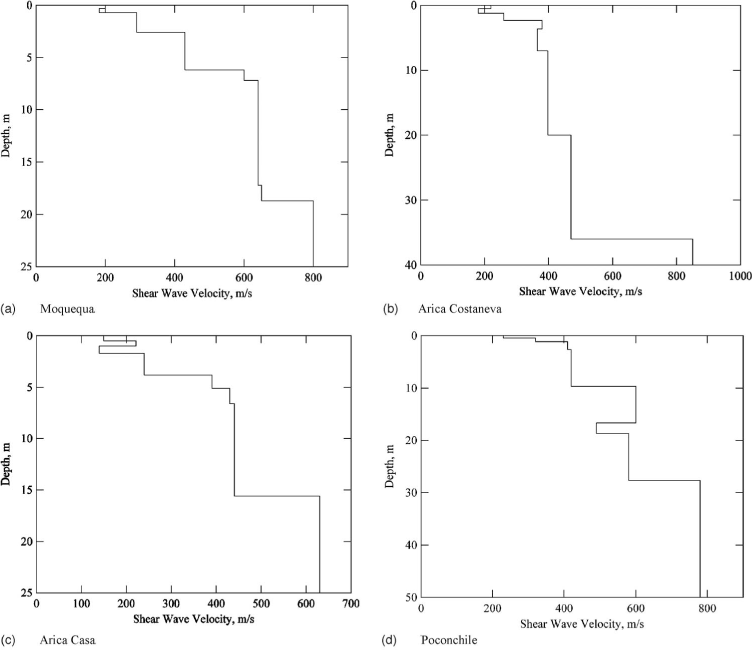
Shear-wave velocity profiles at ground motion sites.
Average shear-wave velocity and site classification at ground motion stations
See
SASW Quality: Level 1—smooth dispersion data.
Level 2—limited jumps in dispersion data.
Level 3—significant jumps in dispersion data or limited depth achieved.
Site period from the peak RRS.
Site period from surface to bedrock shear-wave profile (Bedrock defined as V s > 540 m/s).
V s were measured only to 25 m. V s values for deeper layers were assumed to be equal to the bedrock V s value measured at 25 m.
Based on predominant period from H/V ratios.
Classification based on H/V ratios using the methodology of Zhao et al. (2006a).
Ground Motion Parameters
An evaluation of engineering ground motion parameters of the records obtained in the 2001 Southern Peru earthquake is important given the uniqueness of these records. Ground motions parameters considered in this study include response spectra, ground motion duration, Arias Intensity, and frequency content parameters. Whenever possible, the recorded parameters are compared with existing attenuation relationships.
There exist various ground motion prediction equations (GMPE) for subduction type earthquakes (e.g., Atkinson and Boore 2003 and Youngs et al. 1997, developed from worldwide data; Ruiz and Saragoni 2005, based on Chilean data; McVerry et al. 2006, based on data from New Zealand earthquakes; Zhao et al. 2006b, using data from Japanese earthquakes). The limited number of records obtained in the earthquake precludes any statistically rigorous comparison of predicted and recorded ground motion parameters. Nevertheless, GMPE provide a useful frame of reference for the recorded ground motions. Figure 5 shows the response spectra of the recorded ground motions along with those predicted by the attenuation models of Atkinson and Boore (2003) and Youngs et al. (1997). As noted earlier, the recording sites where shear-wave velocities were measured correspond to IBC Site C soil class and therefore the Atkinson and Boore (2003) relationship for sites of that type and the Youngs et al. (1997) relationship for soil are plotted for consistency. These same data is presented as a function of distance for selected spectral periods in Figure 6. Both horizontal components (North–South and East–West) are generally similar in amplitude, with the East–West component on average about 10% higher across all periods. The horizontal response spectra at Moquegua (Dfault=71 km, Figure 5a) generally fall between the median and the one standard deviations of GMPE. On the other hand, the spectra recorded at Arica (~140 km from the fault, Figure 5b and 5c), and Poconchile (~160 km, Figure 5d) fall at or above the plus one standard deviation predictions of GMPE. In fact, spectral amplitudes decrease little between the Moquegua record (71 km) and the Arica and Poconchile records (~ 150 km), in particular for short spectral periods (Figure 6). As discussed later, the lack of distance attenuation for short spectral periods is not captured by a finite fault simulation of the fault rupture, and can only be partially explained by site response. The spectra recorded at Putre and Cuya (about 190 km from the fault plane, Figure 5e and 5f) both have similar characteristics, with short period spectra significantly higher than the median plus one standard deviation of GMPE. These records, however, have long period spectral accelerations at or below the median value of GMPE. Finally, the Pisagua recording (~220 km from the fault plane) has spectral values near the median minus one standard deviation curve of GMPE. Although no site investigation was conducted at this site, it is believed to be located on a weathered rock outcrop. Figure 6 clearly illustrates how for short spectral periods recorded ground motions are higher than predictive equations for all records between 100 and 200 km from the fault. At longer spectral periods, attenuation becomes significant for the more distant records.
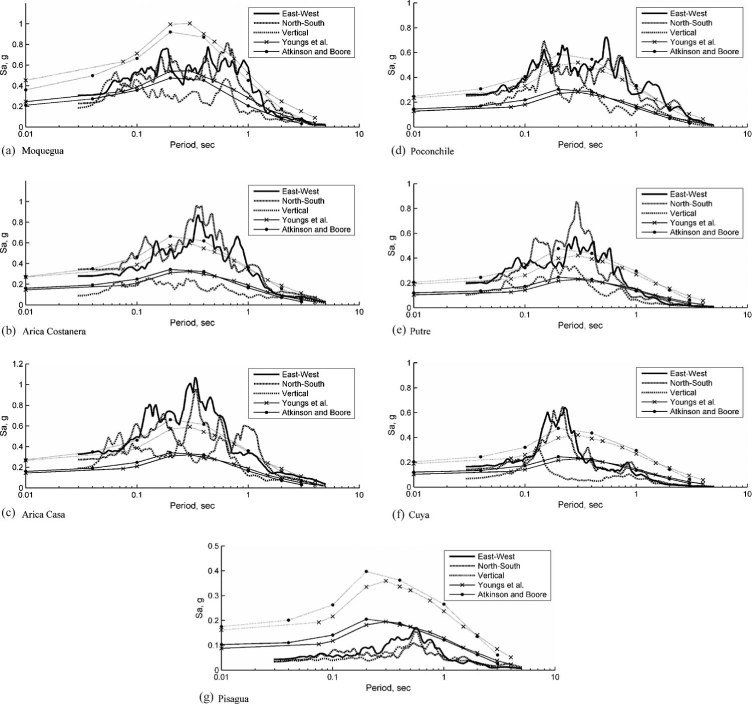
Response spectra (5% damping) of recorded motions. For reference, the median and the 84th percentile predictions of the attenuation relationships of Atkinson and Boore (2003) and Youngs et al. (1997) for Site C and for soil site conditions, respectively, are also shown.
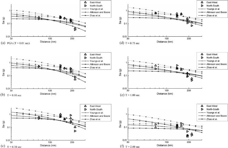
Recorded spectral accelerations (5% damping) plotted as a function of closest distance to the fault. For reference, the median and the 84th percentile predictions of the attenuation relationships of Atkinson and Boore (2003), Youngs et al. (1997), and Zhao et al. (2006b) are also shown. These relationships are plotted for a stiff soil site condition (Site C in Atkinson and Boore and Zhao et al., and soil condition in Youngs et al.)
Single-valued ground motion parameters for the strong motion records are listed in Table 3. Peak ground acceleration decreases with distance for all records except Moquegua (Figure 6a). The same pattern is observed for peak ground velocity (PGV) and displacement (PGD). An exception is noted for the PGD values recorded at Pisagua which are higher than those at closer stations, possibly because of baseline correction errors. Ground motion intensity and energy content can be also quantified by the Arias Intensity (Arias 1970). Figure 7 plots the Arias Intensity (Ia) values computed for the recorded ground motions. Note that the Ia is higher for stations closer to the fault, even though peak ground motion parameters were lower for the Moquegua station than for more distant stations. Figure 7 also includes predicted Ia values based on an attenuation model from Travasarou et al. (2003). This attenuation model was developed without subduction data and thus it is not surprising that the Ia based on the recordings exceed the predicted values, reflecting the fact that subduction zone events, at least in Southern Peru and Chile, can have higher energy contents than records from crustal earthquakes.
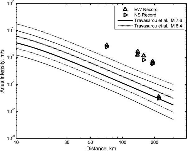
Computed values of Arias Intensity plotted as a function of closest distance to the fault. The predictions of an attenuation relationship by Travasarou et al. (2003) are also shown for comparison (thick lines correspond to the median prediction, thin lines correspond to median plus and minus one standard deviation). The Travasarou et al. relationship is developed with data for shallow crustal earthquakes with Mw 7.6. The dotted line shows an extrapolation to Mw 8.4.
Ground motion parameters for the recorded ground motions
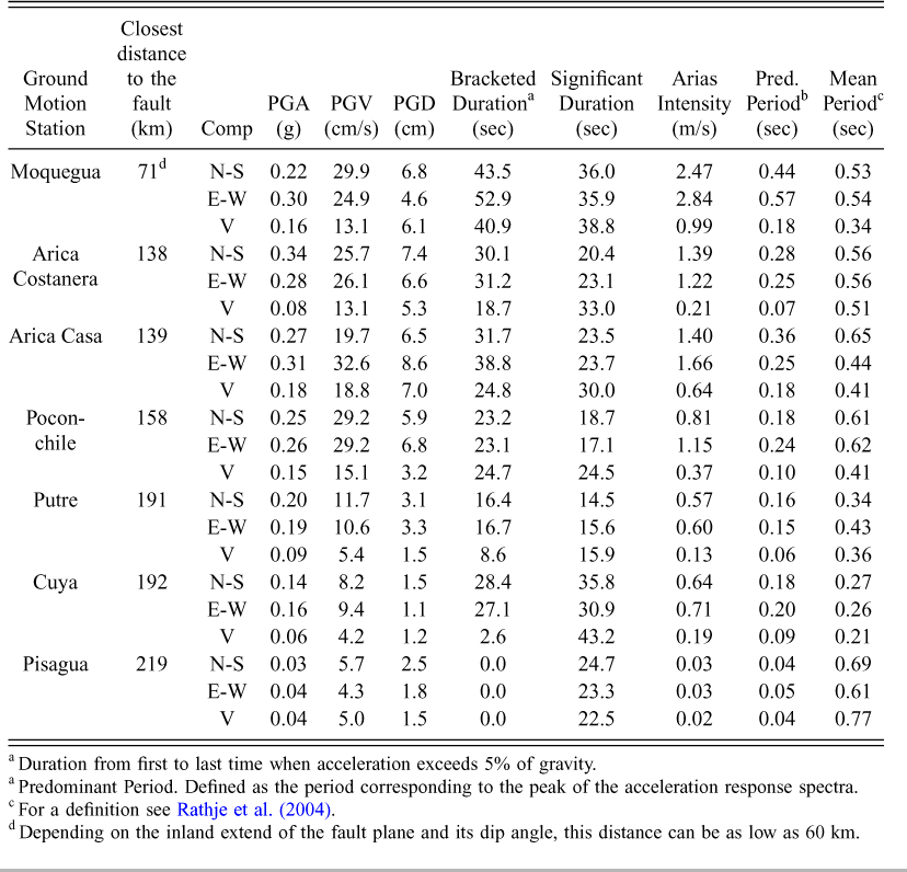
Duration from first to last time when acceleration exceeds 5% of gravity.
Predominant Period. Defined as the period corresponding to the peak of the acceleration response spectra.
For a definition see Rathje et al. (2004).
Depending on the inland extend of the fault plane and its dip angle, this distance can be as low as 60 km.
Ground motion duration is an important parameter when nonlinear analyses are needed. Duration is often quantified by the significant duration (D5–95), which quantifies the time to go from 5% to 95% of the Arias Intensity. Figure 8 plots the recorded ground motion duration for all of the recorded stations. The predictive model by Kempton and Stewart (2006) is also plotted for reference. The Kempton and Stewart (2006) model is developed with data from shallow crustal earthquakes and does not include data from magnitudes larger than Mw 7.6; however, there are no similar relationships for subduction zone earthquakes and the relationships of Kempton and Stewart (2006) is considered useful as a reference value. Observe that there is no clear trend of duration with distance. Moreover, only the Moquegua record (Dfault=71 km) had durations comparable to those predicted by the Kempton and Stewart attenuation model for Mw 7.6 (the upper range of model applicability). Given the large magnitude of the earthquake, the relatively short durations for the recorded ground motions were not expected.
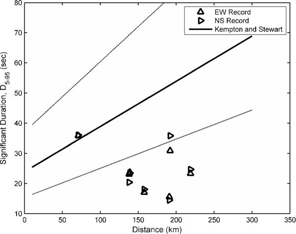
Recorded 5–95% Significant Durations versus distance. The median and plus/minus one standard deviation band predictions of the Kempton and Stewart (2006) attenuation relationship for a Mw 7.6 earthquake (the limit of applicability of that model) are shown for reference.
The Fourier amplitude spectrum or the response spectra represent the frequency content of an earthquake ground motion. Single valued-parameters obtained from either the Fourier amplitude spectrum or the response spectra, such as the predominant period, have also been used to characterize the frequency content of a strong ground motion. Rathje et al. (2004) discuss the relative advantages of these and other single valued parameters used to characterize frequency content, and conclude that mean period (Tm) is both a stable and a representative parameter of frequency content. The values of Tm and other frequency domain parameters of the ground motions recorded in the Southern Peru earthquake are given in Table 3. Rathje et al. (2004) also developed an empirical attenuation relationship for Tm. Figure 9 illustrates the mean period of the recorded ground motions along with the predictive model of Rathje et al. (2004). Because this model was developed without subduction event data, a direct comparison is not possible. However, such a comparison can be illustrative in several respects. Observe that there is no evidence in the recordings from this earthquake of a correlation between Tm and distance. More importantly, the observed Tm values are more then one standard deviation below the prediction of the Rathje et al. (2004) model. This is particularly unusual because this model predicts an increase in period with increasing magnitude. This is an indication that the recordings in this earthquake are particularly rich in high frequency content. An analysis of the high frequency content of these records is presented in Boroschek and Comte (2006).
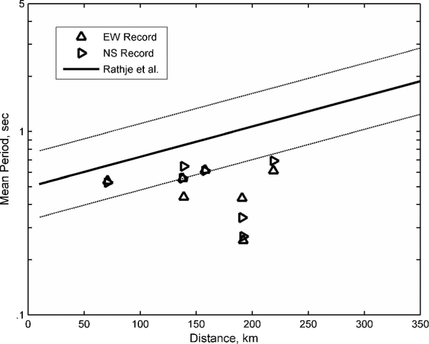
Recorded mean period (Tm). The median and plus/minus one standard deviation band predictions of the Rathje et al. (2004) attenuation relationship are shown for reference.
Site Effects at Ground Motion Stations
Amplification of ground motion due to surficial soil deposits can result in an important contribution to seismic hazard at a site. Empirical studies of site amplification are possible when either a large number of recordings are analyzed such that statistically significant trends between different site conditions can be inferred, or when stations that recorded ground motions in soil are near to stations on bedrock. Neither of these two cases is true for the Southern Peru earthquake. Hence, estimates of the contribution of site response are obtained using the measured shallow shear-wave velocity profiles.
Equivalent linear analysis using SHAKE (Schnabel et al. 1972) is used to predict site amplification at the four ground motion stations where shallow shear-wave velocity profiles were measured (Table 1). Confining stress-dependent modulus reduction and damping versus strain curves were used (EPRI 1993). This was deemed appropriate considering that the soils at the recording sites consist mostly of sands and gravels. Cortez-Flores (2004) performed a sensitivity study using modulus reduction and damping curves proposed by Darendeli for gravels (Darendeli 2001) and found little sensitivity in site response to the choice of these curves.
The absence of recorded bedrock motions in the earthquake implies an absence of valid input motions for use in site response analyses. For this reason, a set of synthetic ground motions was generated using a stochastic finite fault ground motion model (Silva et al. 1990). The model uses published crustal velocity models and a rupture model similar to that of Kikuchi and Yamanaka (2001). The target earthquake ground motions are modeled as a combination of smaller subevent earthquakes occurring over the target rupture plane. This stochastic finite-fault ground motion model was validated by modeling 15 crustal earthquakes recorded at over 500 sites (Silva et al. 1997). The synthetically generated motions were generated both for the ground surface and for an outcropping bedrock with shear-wave velocity value of 800 m/s. This bedrock was encountered at relatively shallow depths for three of the Vs profiles at the ground motion stations (Moquegua, Arica Costanera, and Poconchile). The predicted response spectra at the surface matches relatively well the observed spectra at Moquegua, but is much lower than the recorded spectra at the Chilean stations. Details of these simulations are discussed by Silva et al. (2007).
Site response was quantified by the ratio of response spectra (RRS) between computed surface spectra and the input motion. This parameter permits an estimate of the contribution of site response at different periods, and is less sensitive to the input ground motion than peak ground motion parameters. The uncertainty in input ground motion resulting from the absence of bedrock recordings was captured using 30 different synthetic records generated using the finite fault simulation described above.
The predicted RRS and their uncertainty are shown in Figure 10. The estimated site periods (i.e., the period for highest RRS) are listed in Table 2. These periods are relatively low, as is expected for the relatively stiff profiles. In fact, with the exception of the Arica Costanera station, the measured Vs profiles contribute significantly to site response only for periods lower than about 0.3 s. The Arica Costanera site has relatively lower Vs values and has a clear amplification peak at 0.3 s. Note that a 1-D site amplification analyses does not capture well any resonance due to geological structures deeper than about one quarter wave length of the propagating shear waves.
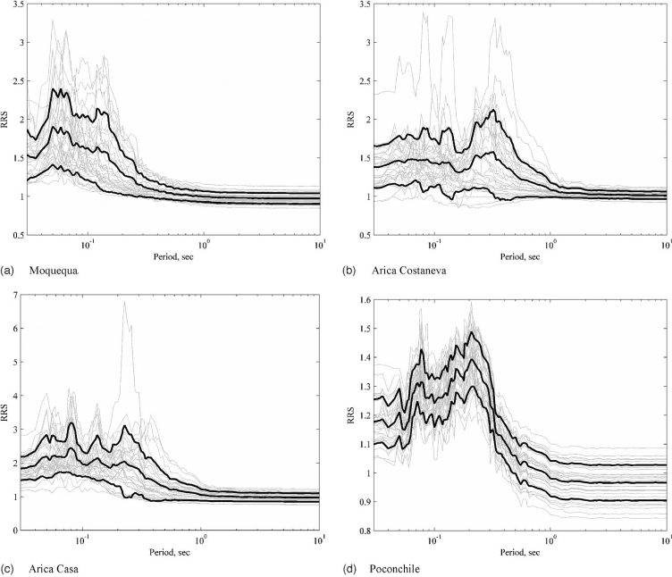
Ratio of response spectra using synthetically generated motions as input motions at ground motion stations sites. Thick lines represent the median and the plus/minus one standard deviation bands obtained from the data.
In order to account for possible measurement errors in the Vs profile, a set of randomly generated shear-wave profiles were obtained by assuming that the measured average Vs of each profile had a normal distribution centered on the recorded value with a coefficient of variation of 6%. This coefficient of variation was reported by Marosi and Hiltunen (2004) and Moss (2008) as a typical SASW measurement error in the average Vs over the upper 30 m. Profiles were then generated by introducing random variability around the Vs profile obtained from the measured dispersion curve, and ensuring that the average Vs maintains a coefficient of variation of 6%. Note that this methodology for generating random profiles assumes no spatial correlation other than the trend given by the measured Vs profile. Moreover, this methodology does not assure that each realization of the Vs profile is compatible with the measured dispersion curve. While this is a simplification, parametric studies showed that the simplified model captured well uncertainties in estimated RRS values.
Figure 11 shows the standard deviations estimated for the Moquegua profile using a set of 30 synthetically generated input motions and 500 randomly generated Vs profiles. To account for the difference between measured and predicted surface response spectra, the outcropping rock ground motions were linearly scaled to match predicted surface peak ground acceleration. The standard deviations were estimated using Monte Carlo simulation with a total of 15,000 runs (500 different Vs profiles for 30 different input motions) for each ground motion station. Observe that the standard deviations are controlled by the uncertainty in input motion and the uncertainty in the measured Vs values does not contribute much to the estimated uncertainty in spectral acceleration.
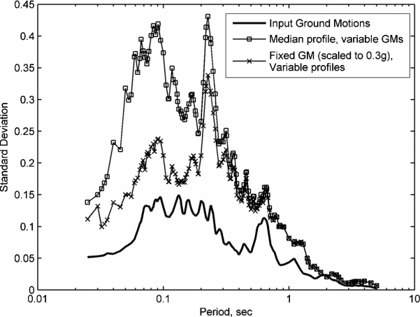
Standard deviations of spectral acceleration (Sa) values considering the contribution of different sources of uncertainty at the Moquegua site.
Other Estimates of Site Response
Single station recording of microtremors or ambient noise are used frequently in practice to estimate site amplification. The methodology initially proposed by Nakamura (1989) is to use the horizontal to vertical (H/V) ratio of Fourier spectra as an estimate of site response (e.g., Lermo and Chavez-Garcia 1993; SESAME 2004). Although uncertainties remain over the validity of the methodology, an extensive research project conducted by a consortium of European Universities (SESAME 2004) concluded that the period corresponding to the peak H/V ratio can render an adequate estimate of the site period if a clear impedance contrasts exists at a site. The reliability of the estimate increases with the sharpness of the peak. Several authors have also used H/V ratios of strong motion recordings to obtain estimates of site response. For example, Zhao et al. (2006a) propose a site classification scheme using the H/V ratio of response spectra of strong motion. Rodriguez and Midorikawa (2003) compared spectral ratio techniques for estimation of site effects using both microtremor data and earthquake ground motions. They conclude that, while less reliable, the H/V ratio of S-wave and coda waves of strong motion data can render estimates of site period similar to H/V ratio of microtremors.
The H/V ratios of strong motion were obtained for four records with sufficiently long recordings to allow for a stable estimate of these ratios. The H/V ratios were obtained from 10 s windows of the recording following the first S-wave arrival. Each FFT component was smoothed using a Parzen window. The H/V ratio was taken as the vector sum of the Fourier spectra of the two horizontal components divided over the vertical component. Finally, the average H/V ratio of all the signal windows was obtained and is plotted in Figure 12.
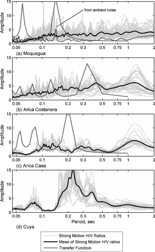
H/V ratios estimated from strong motion data. The thin lines show H/V for individual 10 s windows, the thick lines show the average of all windows. For the Moquegua record, the H/V estimate using ambient noise is also included (Sato and Konagai 2002).The transfer function estimated using equivalent linear analysis for stations with Vs measurements are also shown.
For the Moquegua station, the H/V ratios are not consistent across all the time windows and no clear peak can be discerned. At this station, Sato and Konagai (2002) also performed ambient noise measurements at the ground motion station. The H/V ratios obtained from these measurements are also plotted in Figure 12a. The ratios were obtained following a procedure similar to that described above for strong ground motions, but the time windows were selected by visual examination of both the time and frequency domain of the records in such a way as to minimize noise. There is a clear peak in the ambient noise measurement of H/V ratios at 7 Hz. This peak satisfies the criteria established in SESAME (2004) and hence it is thought to be a good estimate of the site period. This peak also coincides with the theoretical peak obtained from the measured SASW profile (Tsite=0.15 s, see Table 2).
The H/V ratios for the Arica Costanera station (Figure 12b) also lack a clear peak, but the peak at around 0.43 s is relatively close to the peak of the transfer function estimated from site response analysis. The H/V ratios for the Arica Casa station (Figure 12c) shows a broadband peak at around 0.12 seconds. This peak does not coincide with a peak in the RRS. Contrary to the other three stations, the H/V ratios at Cuya show a clear peak at 0.22 seconds (Figure 12d). This peak is common to all time windows (both during strong motion and the later, less intense part of the spectrum). The strong resonance indicates the possible presence of a well defined impedance contrast.
Discussion
Predicted site amplification at stations where shear-wave velocities were measured is high for short periods and practically nonexistent at periods longer than one second (Figure 10). The high amplifications at short periods are the result of predicted resonances in very shallow layers (e.g., the top layers in Figure 4 with depths lower than 5 m). While the predicted amplification is not high (an RRS of about 2.0), resonances for such shallow layers are likely over predicted by one-dimensional amplification since damping at very low confining stresses for granular soils are likely higher than those measured by conventional tests. The large spectral accelerations of recorded ground motion up to about 1 second spectral period, and the suggestion of possible longer period peaks in the H/V ratios, indicate the likely contribution to site response of deeper structures. In fact, a salient limitation of 1-D analyses of stiff sites is that resonances due geological structures deeper than the measured profile are not captured by the analyses. In the case of the profiles studied herein, it implies that RRS for periods above 0.3 seconds for Moquegua, Arica Casa, and Poconchile, and about 0.5 seconds for Arica Casa, may not reflect actual site response at the site.
The average amplification over the short period and intermediate period bands used to develop the Fa and Fv site amplification factors in the IBC building codes (ICC 2006) were estimated using the Monte Carlo simulations described above. These amplification factors are compared to those of the IBC and those proposed by Rodriguez-Marek et al. (2001) for similar site conditions (Site C, as classified by the IBC) based on an empirical analyses of the recordings of the Loma Prieta and Northridge earthquakes (Table 4). Observe that long period amplification factors (Fv) are largely underestimated by the 1-D site response analyses at the ground motion sites. On the other hand, the short period amplification estimated for these sites are larger than code values and an average are similar to those observed in the Loma Prieta and Northridge earthquake for similar site conditions (Rodriguez-Marek et al. 2001, Borcherdt 2002). This reinforces the fact that IBC Fa factors for site C (very stiff soils) are underestimated by the current code.
Comparison of amplification factors for IBC Type C sites (ICC 2006). Values in parentheses show computed range of RRS values.
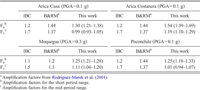
Amplification factors from
Amplification factors for the short period range.
Amplification factors for the mid period range.
Implications for Seismic Hazard Analyses
As shown in Figure 6, existing attenuation relationships largely underpredicted short period spectral accelerations. In part, the large intensities at short periods can be explained by 1-D site amplification. The effect of 1-D site amplification on spectral accelerations can be captured by the estimated RRS bands shown in Figure 10. That is, the recorded spectral accelerations divided by estimated RRS values constitute an estimate of bedrock motions. Figure 13 compares the estimated bedrock acceleration with GMPE for rock. Note that while site response does explain some of the amplification, ground motions are still higher than those predicted by attenuation relationships.
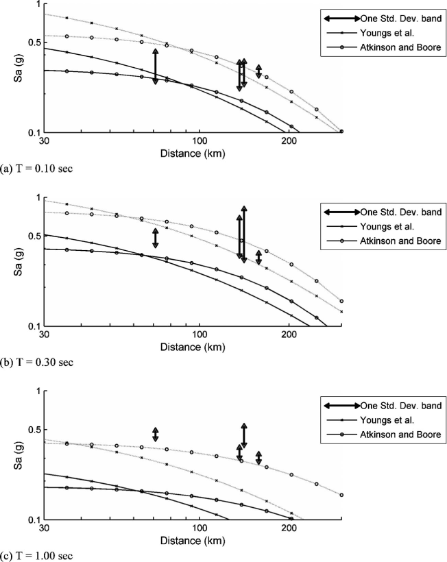
Estimated spectral accelerations for a rock site condition (5% damping) plotted as a function of closest distance to the fault. The bands represent the uncertainty resulting from the contribution of site response. For reference, the attenuation relationships for rock of Atkinson and Boore (2003) and Youngs et al. (1997) are also shown.
The ground motions recorded in the Southern Peru earthquake are unique in that no strong motions for similar magnitude earthquakes exist to date. Ground motion time histories are often required for nonlinear analysis of important structures. Considering that in Alaska and the Pacific Northwest region of the United States large megathrust earthquake contribute to hazard, the Southern Peru recordings are likely to be sought after when time histories are required. It is important that the engineer considers the important contribution of site response at high frequencies when using these motions, given that it is unlikely that the same site effects contribution would be present at sites in the Pacific Northwest and Alaska. Moreover, as discussed in the Ground Motion Parameters section, the Chilean recordings have an unusually short duration for such a large magnitude earthquake.
Conclusions
The 23 June 2001 Mw 8.4 Southern Peru earthquake was the largest seismic event recorded by a strong motion seismograph network. The earthquake produced seven high quality free-field accelerographs measured within 250 km of the causative fault. The scarcity of strong ground motion records for megathrust earthquakes makes these recordings unique and highly valuable to seismic design engineers practicing in and near active subduction zones. Shear-wave velocities were measured at four of the ground motion stations that recorded the earthquake revealing stiff soil profiles (IBC C sites) with Vs increasing rapidly with depth to values greater than 600 m/s. Engineering analysis of the accelerographs indicate that although having been recorded at stiff soil sites, site amplification appears to have contributed to the recorded motions, particularly at short periods, due to resonances within shallow layers of soil. In general, short period spectral amplitudes (T<0.5 s) show limited attenuation with distance. In contrast, a significant attenuation of long period energy is observed in the recordings for distances greater than about 160 km. Arias Intensity (Ia) values attenuates with distance for all records; however, no correlation between mean period (Tm) and distance was found.
Comparing the recording motions with GMPE indicates that the current attenuation relationships largely underpredicted short period spectral accelerations. This is due in part to 1-D site amplification in this period range. More generally, GMPE were found to underpredict the observed ground motions at all periods for distances ranging from 100 km to 200 km. The average amplification over the short- and intermediate-period bands used to develop the Fa and Fv site amplification factors in the IBC building codes (ICC 2006) were estimated in a series of Monte Carlo 1-D ground response simulations. These analysis results indicate that short period amplification (Fa) estimated for these sites are larger than code values and on average are similar to those observed in the Loma Prieta and Northridge earthquake for similar site conditions (Rodriguez-Marek et al. 2001; Borcherdt 2002). This reinforces the fact that IBC Fa factors for site C (very stiff soils) are underestimated by the current code.
It is expected that ground motions recorded in the Southern Peru earthquake will play a role in development of future GMPE and find use for time-history structural and geotechnical engineering analyses in area where megathrust earthquakes contribute to the seismic hazard, such as Alaska and the Pacific Northwest regions of the United States, and through much of the west coast of Central and South America and Japan. It is important that engineers consider the important contribution of site response at high frequencies when using these motions, given that it is unlikely that the same site effects contribution would be present at all sites. Moreover, it should be recognized that the Chilean recordings have an unusually short duration considering the large magnitude of the earthquake.
Footnotes
Acknowledgments
This material is based on work supported by the National Science Foundation under Grants No. CMS-0130617. and CMS-0201574. Any opinions, findings and conclusions or recommendations expressed in this material are those of the authors and do not necessarily reflect the views of the National Science Foundation. Dr. Jorgen Johansson and Paola Mayorca, of the University of Tokyo, facilitated the microtremor measurements at the Moquegua station. The Peru–Japan Center for Seismic Investigation (CISMID) facilitated the recorded ground motion at Moquegua. Their contribution is greatly appreciated.