Design Seismic Demands from Seismic Response Analyses: A Probability-Based Approach

Abstract

Earthquake-resistant design guidelines commonly prescribe that when conducting seismic response analyses: (i) a minimum of three ground motions can be used; (ii) if less than seven ground motions are considered, the maximum of the responses should be used in design; and (iii) if seven or more ground motions are considered the average of the responses should be used in design. Such guidelines attempt to predict the mean seismic response from a limited number of analyses, but are based on judgment without a sound, yet pragmatic, theoretical basis. This paper presents a rational approach for determining design seismic demands based on the results of seismic response analyses. The proposed method uses the 84^th percentile of the distribution of the sample mean seismic demand as the design seismic demand. This approach takes into account: (i) the number of ground motions considered; (ii) how the ground motions are selected and scaled; and (iii) the differing variability in estimating different types of seismic response parameters. A simple analytic function gives a ratio which, when multiplied by the mean response obtained from the seismic response analyses, gives the value to be used in design, thus making the proposed approach suitable for routine design implementation.

Introduction

The consistent determination of design seismic demands on structures and other engineered facilities via seismic response analyses requires the consistent development and implementation of: (i) “target” ground motion intensity measures and/or seismic response spectra for ground motion selection; (ii) consistent selection of ground motion records in accordance with this “target”; and (iii) consistent interpretation of the results of the seismic response analysis using the selected ground motions for seismic design. This manuscript deals solely with the latter of the above three points, but it must be made clear that without the former two, consistent seismic design via the use of seismic response analyses cannot be achieved.

Variability in seismic response analyses using different input ground motions which match some predetermined “target” intensity measure (e.g., spectral acceleration response spectra) occurs because both the system response and input ground motion are significantly more complex than the simple “target” intensity measure upon which the ground motions are selected. Just as uncertainties are explicitly accounted for in probabilistic seismic hazard analysis (PSHA; Cornell 1968, SSHAC 1997), from which “target” ground motion intensity measures and design response spectra are commonly obtained, uncertainties also need to be considered in seismic response. In rigorous performance assessments, this “record-to-record variability” in seismic response as well as many other uncertainties are typically explicitly accounted for (Cornell et al. 2000). Conversely, in less rigorous assessments, the aim is typically to use seismic response analysis results to obtain a deterministic measure of seismic demand for the design and/or simple verification of different components in the system.

Modern seismic design guidelines recognize the variability in seismic demands estimated using seismic response analysis with different input ground motions. Typically such guidelines (e.g., Eurocode 8, Part 1 (CEN 2003), FEMA 368 2001, ASCE 7-05 2006, ASCE 4-98 2000, NZS1170.5 2004) state one or more of the following points in the presence of this variability: (i) a minimum of three ground motions should be considered; (ii) if less than seven ground motions are considered then the maximum response should be considered; and (iii) if seven or more records are considered, the average demand may be adopted. Clearly the above guidelines, which are based on engineering judgement, seek to estimate (sometimes conservatively) the mean seismic demand, despite the fact that this mean seismic demand is estimated from a limited number of plausible ground motions.

The above guidelines have however several important deficiencies in their use in engineering design: (i) they address variability in seismic response in a deterministic manner and as a result it is not clear, for example, what is the likelihood that the maximum of three seismic response analyses is smaller than the “true” mean seismic response; (ii) they provide no explicit incentive for conducting larger (i.e., greater than seven) numbers of seismic response analyses, something which is now routinely possible considering the time to conduct analysis versus the time to develop and validate a seismic response model; (iii) they do not directly provide any motivation for reducing uncertainty in seismic response analyses by careful ground motion selection (Baker et al. 2006, Bradley et al. 2009a, Hancock et al. 2008); and (iv) they do not account for the fact that some measures of seismic response are significantly more sensitive to the input ground motion than others (i.e., have a higher variability; e.g., Hancock et al. 2008).

This manuscript presents a simple method for determination of seismic demands based on the distribution of the sample mean of the seismic response analyses. Firstly, the unknown likelihood in the conventional approach, that the maximum of three seismic response analyses is less than the “true” seismic demand, is examined. Secondly, the proposed methodology based on the distribution of the sample mean is discussed and it is explained how it accounts for the four aforementioned deficiencies of the current approach. A simple analytic expression is then derived which can be used to obtain the design seismic demand by combining it with the estimated mean seismic demand.

Estimation of the Mean Seismic Demand

As previously mentioned, design guidelines are interpreted to focus on the estimation of the average seismic demand (Baker et al. 2006, Hancock et al. 2008, Watson-Lamprey 2006). There are three such measures of “average” which are used in earthquake engineering: the arithmetic mean, the geometric mean and the median. Hancock et al. (2008) mention that based on presentations by, and discussions with, U.S. code drafters, it is clear that the arithmetic mean is the intended definition of “average” used. For this reason, the term “average seismic response” or “mean seismic response” in the remainder of this manuscript refers to the arithmetic mean seismic response. It should also be noted that for any given set of observations (which have positive skewness) the arithmetic mean will always be larger than the geometric mean.

Another premise in the analysis conducted in this manuscript is that variability in seismic demand due to different input ground motions can be represented by a lognormal distribution. This assumption has been widely demonstrated to be statistically justified, for example in Shome and Cornell (1999),Aslani and Miranda (2005), Mander et al. (2007), and Bradley et al. (2009b), among others. The lognormal distribution is also desirable in that it is completely defined by its first two moments, μ_lnX and $σ_{\ln X}^{2}$ . A result of the lognormal assumption is that:

μ_{X} = \exp (μ_{\ln X} + σ_{\ln X}^{2} / 2)

(1)

where μ_X is the arithmetic mean of X; and exp(μ_lnX), the exponential of the arithmetic mean of lnX, is equal to the geometric mean and median of X (i.e., the arithmetic mean is greater than the geometric mean). It is also noted that the lognormal standard deviation, σ_lnX, is frequently referred to as the “dispersion,” and given the symbol β_lnX, although it will not be done so here.

If a limited number of ground motions are considered (from a potentially infinite number of plausible motions) in seismic response analyses, then the estimation of the mean seismic demand based on this limited number of analyses is uncertain. Figure 1a illustrates a lognormal probability density of some measure of seismic demand, denoted as X. Also shown are values of X obtained from seven seismic response analyses (denoted as “random realisations” in Figure 1a. From these seven realisations of X the sample mean of X can be computed, as an approximation of the true mean of X (which in general is unknown, but is 0.02 in this example), as shown in Figure 1b. By repeating such computations for different sets of seven realisations the probability mass function of the sample mean in Figure 1b can be obtained. For the particular realisation shown in Figure 1, it is observed that the sample mean is smaller than the “true” mean of X.

Figure 1

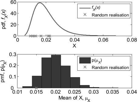
Illustration of the uncertainty in the prediction of the sample mean of X: (a) probability density function (pdf) of X and random realizations; and (b) probability mass function (pmf) of the sample mean of X and one realization.

In order to understand the factors influencing the distribution of the arithmetic sample mean of X (where X is a lognormal random variable), a similar problem for which an analytical solution is possible is considered. In the case of estimating the sample mean of lnX, where X has a lognormal distribution with known variance, $σ_{\ln X}^{2}$ , it can be analytically shown that the sample mean of lnX has a normal distribution with mean equal to the “true” (i.e., population) mean, μ_lnX, and variance equal to the “true” variance divided by the number of independent samples, $σ_{\ln X}^{2} / N$ (e.g., Ang et al. 2007). Therefore, the uncertainty in the sample mean of lnX is dependent on both uncertainty in lnX itself, $σ_{\ln X}^{2}$ , and also the number of independent samples, N. The case of unknown $σ_{\ln X}^{2}$ is elaborated upon later in the manuscript.

In the case of determining the distribution of the arithmetic sample mean of X (which has a lognormal distribution), as is the case of interest here, no simple analytic solution is possible, although several approximations have been attempted (Lam et al. 2006, Lord 2006). Thus in the remainder of this manuscript Monte Carlo simulation, similar to that discussed with reference to Figure 1 is adopted. The analytical result presented in the previous paragraph is used to understand the variation in parameters that is necessary in the Monte Carlo simulations.

Distribution of the Maximum of Three Response Analyses

As previously mentioned, many seismic design guidelines specify that the seismic demands on a system can be estimated based on the maximum of as little as three seismic response analyses. In this section, the ratio of the maximum of three seismic response analyses to the “true” mean seismic demand is investigated.

Monte Carlo simulation was used to examine the distribution of the maximum of three seismic response analyses as follows: (1) given a seismic demand measure, X, with prescribed lognormal mean and standard deviation, μ_lnX and σ_lnX, respectively, generate a sample of three random realisations, x_i1,x_i2,x_i3; (2) take the maximum of these random realisations and divide by the mean (μ_X), i.e., R_i=max(x_i1,x_i2,x_i3)/μ_X; (3) repeat steps (1) and (2) N_sim number of times; and (4) with the N_sim R_i values form an empirical cumulative distribution function (CDF) of R_i.

A value of R_i < 1 represents the case of interest here in which the maximum seismic demand from three seismic response analyses is less than the “true” mean seismic demand, μ_X. Also, because of the normalisation by μ_X in the definition of R_i it can be shown that R_i is independent of μ_X. Therefore one needs only to examine the effect of the lognormal standard deviation, σ_lnX, on R_i. Figure 2 illustrates the empirical CDFs of R_i for various values of σ_lnX. The empirical CDFs shown were obtained based on N_sim = 50,000 Monte Carlo simulations. It can be seen that, as would be expected, the distribution of R_i is a function of σ_lnX. Furthermore, the cumulative probability of R_i < 1 is also a function of σ_lnX. That is, the probability of the maximum of three seismic response values being less than the “true” mean seismic response depends on the lognormal standard deviation of the response measure. For a lognormal standard deviation range of σ_lnX = 0.2–0.8, Figure 2 illustrates that this probability ranges from 0.15–0.28. Thus, over this reasonable range of σ_lnX the probability of the maximum of three seismic response analysis results being less than the underlying mean varies by a factor of 2. If one examines a “very uncertain” seismic demand measure then the probability of R_i < 1 increases further. For example, in the case of column fatigue damage, which Hancock et al. (2008) find for one application has σ_lnX = 1.232, the probability of R_i < 1 is approximately 0.4 (i.e., a 40% chance that even the maximum of three samples is less than the true mean).

Figure 2

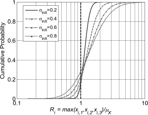
Distribution of the ratio of the maximum of three random realisations to the arithmetic mean of a lognormal distribution for various lognormal standard deviations.

Clearly such a variable probability of R_i < 1 is undesirable and is a shortcoming of the current design prescriptions. The method for determination of seismic demands via seismic response analysis proposed in the following section, by definition, has a fixed probability that the design seismic demand is less the “true” mean value.

Determination of Seismic Demand Values Using the Distribution of the Sample Mean

It is proposed here that the distribution of the sample mean obtained from the results of seismic response analyses be used to determine the design seismic demand. This proposal is based on the fact that, as previously mentioned, current code guidelines are oriented toward the prediction of the mean seismic demand. It is further proposed that the 84^th percentile of the distribution of the sample mean is used as the design seismic demand. Why the 84^th percentile in particular? The use of the 84^th percentile of a distribution has frequently been used to obtain deterministic design values in related topics such as seismic hazard analysis. Also, while it is by no means a reason for adopting the 84^th percentile, it is noted that such a proposal gives a constant 16% probability of the design seismic demand being less than the true mean seismic demand. This probability of exceedance is comparable to the 15%-28% observed in Figure 2, relating to the maximum of three responses. Thus, it is envisaged that the use of a larger percentile (e.g., the 95^th percentile) would be overly conservative relative to current approaches.

The proposal of using the 84^th percentile of the sample mean as the design seismic demand has several repercussions. These repercussions are examined in detail in this section, however they are immediately stated here in response to the limitations of conventional seismic design guidelines discussed in the introduction:

i) The method is based on probability theory. Hence, there is a known likelihood of the true mean being above the design value (equal to 16% if the 84^th percentile is adopted as proposed herein).

ii) As shown in Equation 4 and Figure 3 to follow, the standard deviation of the distribution of the sample mean reduces (and hence so does the ratio of the 84^th percentile relative to the “true” mean) as the number of ground motions used in seismic response analyses increases. As a result there is a clear benefit of performing additional seismic response analyses.

Figure 3

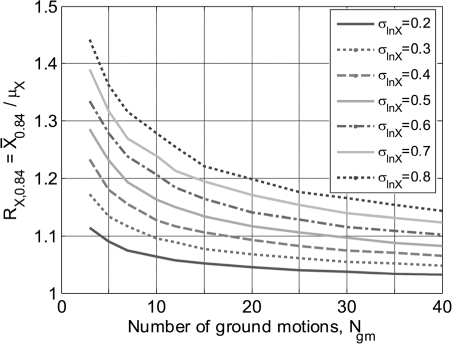
Ratio of the 84^th percentile of the distribution of the sample mean to the underlying true (i.e., population) mean as a function of the lognormal standard deviation and number of ground motions considered.

iii) As shown in Equation 4 and Figure 3, the ratio of the 84^th percentile of the sample mean to the “true” mean reduces with reducing uncertainty in the results of seismic response analyses. There is therefore a clear benefit of reducing uncertainty in the results of seismic response analyses via “careful” ground motion selection (e.g., Baker et al. 2006, Bradley et al. 2009a, Hancock et al. 2008).

iv) The influence of uncertainty in the results of seismic response analyses on the ratio of the 84^th percentile of the sample mean to the “true” mean, R_X,0.84, also means that the proposed method accounts for the fact that some seismic response measures are more uncertain than others (e.g., Hancock et al. 2008).

84^TH PERCENTILE SAMPLE MEAN DISTRIBUTION RATIO

To illustrate the implications of the procedure described above Monte Carlo simulation was used. Based on the theoretical distribution of the sample mean of lnX previously discussed, the influential parameters in defining the distribution of the sample mean of X are: μ_X and σ_lnX (which uniquely define the lognormal distribution of X) and the number of ground motions (i.e., independent observations), N_gm. In order to reduce the number of influential parameters the variable R_X,0.84, defined as the ratio of the 84^th percentile of the distribution of the sample mean (denoted as X¯_0.84) divided by μ_X itself, i.e., R_X,0.84=X¯_0.84/μ_X was examined. It was verified by Monte Carlo simulations that R_X,0.84 is independent of the value of μ_X.

The Monte Carlo procedure to investigate the dependence of R_X,0.84 on σ_lnX and N_gm was therefore: (1) given μ_X, σ_lnX and assuming a lognormal distribution, generate N_gm random values X_i,1,…,X_i,Ngm and determine the sample mean, X¯_i; (2) repeat step (1) N_sim times and form an empirical CDF of X¯ _i from which the 84^th percentile, X¯_0.84, can be identified and divided by μ_X to obtain R_X,0.84; (3) repeat steps (1) and (2) for all σ_lnX, N_gm values of interest.

Figure 3 illustrates the results of the Monte Carlo simulation procedure described above (N_sim = 50,000) to determine R_X,0.84 over the range 0.2 ≤ σ_lnX ≤ 0.8 and 3 ≤ N_gm ≤ 40. It can be seen that, as one would expect, the variable R_X,0.84 increases with increasing σ_lnX and reduces with increasing N_gm.

Uncertainty in the Sample Standard Deviation

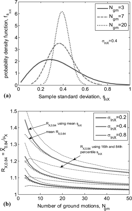
The use of Figure 3 to determine R_X,0.84 requires a value of σ_lnX to be specified. However, in practice the exact value of σ_lnX is not known, and must be estimated from the sample standard deviation, s_lnX. Given that that quotient, $(N_{g m} - 1) s_{\ln X}^{2} / σ_{\ln X}^{2}$ has a Chi Square distribution (Ang et al. 2007), Figure 4a illustrates the distribution of s_lnX for three values of N_gm, given the “true” standard deviation σ_lnX = 0.4,. It can be seen that for small N_gm there is significant variability in s_lnX and the distribution is positively skewed, both of which reduce as N_gm increases.

Figure 4

(a) The distribution of the sample standard deviation for various numbers of ground motions records; and (b) the effect of uncertainty in the sample standard deviation on the ratio of the 84^th percentile of the distribution of the sample mean to the underlying true (i.e., population) mean.

Figure 4b illustrates the effect of the uncertainty in s_lnX on the computed value of R_X,0.84 for σ_lnX = 0.2, 0.4, and 0.8. For each value of σ_lnX, R_X,0.84 was computed using (i) the mean value of s_lnX (i.e., Figure 3); (ii) the 16^th and 84^th percentiles of s_lnX; and (iii) the mean value of R_X,0.84 obtained by numerically evaluating the integral:

E [R_{\ln X, 0.84}] = \int R_{\ln X, 0.84} (s_{\ln X}) f_{s_{\ln X}} d s_{\ln X}

(2)

where f_{s
_lnX} is the probability density function of s_lnX (i.e., Figure 4a). It can be seen that the effect of uncertainty in s_lnX increases as the number of ground motions reduces, and that the mean value of R_X,0.84 is less than the value of R_X,0.84 obtained using the mean value of s_lnX. Because the mean value of R_X,0.84 explicitly accounts for the uncertainty in s_lnX, it is used in the remainder of this manuscript.

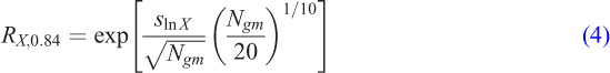
Approximation of R_X,0.84 BY SIMPLE PARAMETRIC EQUATIONS

To make the results discussed in the previous sections more easily applied in a design environment it is desirable to have a mathematical expression of the mean of R_X,0.84 as a function of s_lnX and N_gm. In order to provide theoretical robustness of such an expression use is made of the theoretical solution of the distribution of the sample mean of lnX when σ_lnX is known (not the sample mean of X for unknown σ_lnX that is considered here). As previously mentioned, the distribution of $\bar{\ln X}$ is normal (for X lognormal with known σ_lnX) and hence the ratio of the exponent of the 84^th percentile estimate of the sample mean to the exponent of the true mean is given by (recall that exp[μ_lnX] is the geometric mean of X):

\begin{array}{l} R_{\ln X, 0.84} = \frac{\exp [{\bar{\ln X}}_{0.84}]}{\exp [μ_{\ln X}]} \\ = \frac{\exp [μ_{\ln X} + Φ^{- 1} (0.84) σ_{\bar{\ln X}}]}{\exp [μ_{\ln X}]} \\ = \exp [\frac{σ_{\ln X}}{\sqrt{N}}] \end{array}

(3)

where

{\bar{\ln X}}_{0.84}

is the 84^th percentile of the distribution of

\bar{\ln X}

; Φ⁻¹(0.84) is the inverse standard normal CDF (Ang et al. 2007) evaluated at 0.84 (which is approximately 1.0); and

σ_{\bar{\ln X}} = σ_{\ln X} / \sqrt{N}

is the standard deviation of

\bar{\ln X}

Based on the analytical expression of R_lnX,0.84 given in Equation 3, a similar functional form for the mean value of R_X,0.84 was sought. It was found that the following equation provides an adequate compromise between accuracy and simplicity:

R_{X, 0.84} = \exp [\frac{s_{\ln X}}{\sqrt{N_{g m}}} {(\frac{N_{g m}}{20})}^{1 / 10}]

(4)

Figure 5a illustrates a comparison between Equation 4 and the mean value of R_lnX,0.84 obtained from Monte Carlo simulation, while Figure 5b illustrates the error in the approximation. The additional factor in Equation 4 (compared to Equation 3) was primarily selected to match the Monte Carlo simulation results over the region 5 < N_gm < 25, as evident with an increase in the error ratio for N_gm = 3 in Figure 5b. These errors, which are less than 3% for s_lnX < 0.6 and for N_gm = 3, and less than 1% for N_gm > 7 are considered insignificant relative to other seismic design assumptions, and thus Equation 4 provides a simple parametric fit for R_X,0.84 useful for design.

Figure 5

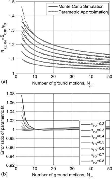
Accuracy of the parametric fit given by Equation 4: (a) plotted against the mean value of R_X,0.84 from the Monte Carlo simulations; and (b) the error ratio compared with Monte Carlo simulation.

Procedure to Obtain Design Seismic Demands

Using the results and discussion in the previous sections the proposed procedure for determination of design seismic demands in a serial fashion is.

Step 1: Based on a pre-determined N_gm ground motion records perform N_gm seismic response analyses using the numerical model of the system.

Step 2: From the N_gm seismic response analyses obtain the values of one or more seismic demand parameters of interest, (i.e., X₁,…,XN_gm for each response parameter of interest). Compute the arithmetic sample mean, X¯, and lognormal standard deviation, $s_{\ln X}$ , of the responses, as given by Equations 5 and 6:

\bar{X} = \frac{1}{N_{g m}} \sum_{i = 1}^{N_{g m}} X_{i}

(5)

s_{\ln X} = \sqrt{\frac{1}{N_{g m} - 1} \sum_{i = 1}^{N_{g m}} {(\ln X_{i} - \bar{\ln X})}^{2}}

(6)

Step 3: Compute R_X,0.84 as given by Equation 4 and then obtain the design seismic demand from Equation 7:

X_{d e s i g n} = \bar{X} R_{X, 0.84}

(7)

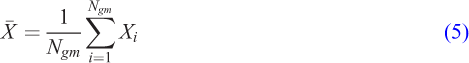
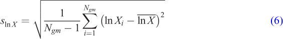
It should be noted that Equations 5 and 6 are “built-in” functions in most programs used in a engineering design environment. For example, “AVERAGE()” and “STDEV()” are the Microsoft Excel functions used for executing Equations 5 and 6. Therefore the three steps outlined above require the same amount of effort as determination of the maximum and average values which are required by the aforementioned design guidelines.

Conclusions

This paper has presented a rational, probability-based approach for determining design seismic demands based on the results of seismic response analyses. The proposed method uses the 84^th percentile of the distribution of the sample mean as the design seismic demand. The method therefore takes into account: (i) the number of ground motions considered; (ii) how the ground motions are selected and scaled; and (iii) the differing variability in estimating different types of seismic response parameters. A simple three-step procedure was explained by which the design seismic demand can be obtained using the proposed approach, thus making it suitable for routine design implementation.

References

Ang

A. H. S.

, and Tang

W. H.

, 2007. Probability Concepts in Engineering: Emphasis on Applications in Civil and Environmental Engineering. John Wiley & Sons, New York, 420 pp.

American Society of Civil Engineers (ASCE), 2000. Seismic Analysis of Safety-Related Nuclear Structures and Commentry.

American Society of Civil Engineers (ASCE), 2006. Minimum Design Loads for Buildings and Other Structures.

Aslani

, and Miranda

, 2005. Probability-based seismic response analysis, Engineering Structures 27, 1151–1163.

Baker

J. W.

, and Cornell

C. A.

, 2006. Spectral shape, record selection and epsilon, Earthquake Engineering and Structural Dynamics 35, 1077–1095.

Bradley

B. A.

, Dhakal

R. P.

Cubrinovski

, and MacRae

G. A.

, 2009a. Prediction of spatially distributed seismic demands in structures: from structural response to loss estimation, Earthquake Engineering and Structural Dynamics 39, 591–613.

Bradley

B. A.

, Dhakal

R. P.

, Cubrinovski

R. P.

, Cubrinovski

, and MacRae

G. A.

, 2009b. Prediction of spatially distributed seismic demands in structures: ground motion and structural response, Earthquake Engineering and Structural Dynamics 39, 501–520.

Cornell

C. A.

, 1968. Engineering seismic risk analysis, Bulletin of the Seismological Society of America 58, 1583–1606.

Cornell

C. A.

, and Krawinkler

, 2000. Progress and challenges in seismic performance assessment, PEER Center News 3, 1–3.

10.

European Committee for Standardization (CEN), 2003. Eurocode 8: Design of Structures for Earthquake Resistance, Part 1: General rules, seismisc actions and rules for buildings, Brussels.

11.

Federal Emergency Management Agency (FEMA 368), 2001. NEHRP Recommended Provisions for Seismic Regulations for New Buildings and Other Structures, 2000 Edition, Part 1: Provisions, Washington, D.C.

12.

Hancock

, Bommer

J. J.

, and Stafford

P. J.

, 2008. Numbers of scaled and matched accelerograms required for inelastic dynamic analyses, Earthquake Engineering and Structural Dynamics 37, 1585–1702.

13.

Lam

C. L. J.

, and Le-Ngoc

, 2006. Estimation of typical sum of lognormal random variables using log shifted gamma approximation, Communications Letters, IEEE, 10, 234–235.

14.

Lord

, 2006. Partially exact and bounded approximations for arithmetic Asian options, Journal of Computational Finance 10, 1–52.

15.

Mander

J. B.

, Dhakal

R. P.

, Mashiko

, and Solberg

K. M.

, 2007. Incremental dynamic analysis applied to seismic financial risk assessment of bridges, Engineering Structures 29, 2662–2672.

16.

Senior Seismic Hazards Analysis Committee (SSHAC), 1997. Recommendations for probabilistic seismic hazard analysis: Guidance on uncertainty and use of experts, U.S. Nuclear Regulatory Commission, U.S. Dept. of Energy, Electric Power Research Institute.

17.

Shome

, and Cornell

C. A.

, 1999. Probabilistic Seismic Demand Analysis of Nonlinear Structures, Ph.D. Thesis, Stanford University.

18.

Standards New Zealand (NZS 1170.5), 2004. Structural Design Actions, Part 5: Earthquake actions - New Zealand. Standards New Zealand, Wellington, New Zealand.

19.

Watson-Lamprey

, 2006. Selection of ground motion time series and limits on scaling, Soil Dynamics and Earthquake Engineering 26, 477–482.

Design Seismic Demands from Seismic Response Analyses: A Probability-Based Approach

Abstract

Introduction

Estimation of the Mean Seismic Demand

Distribution of the Maximum of Three Response Analyses

Determination of Seismic Demand Values Using the Distribution of the Sample Mean

84TH PERCENTILE SAMPLE MEAN DISTRIBUTION RATIO

Uncertainty in the Sample Standard Deviation

Approximation of RX,0.84 BY SIMPLE PARAMETRIC EQUATIONS

Procedure to Obtain Design Seismic Demands

Conclusions

References

84^TH PERCENTILE SAMPLE MEAN DISTRIBUTION RATIO

Approximation of R_X,0.84 BY SIMPLE PARAMETRIC EQUATIONS