Consistent Source-to-Site Distance Metrics in Ground-Motion Prediction Equations and Seismic Source Models for PSHA

Introduction

Ground-motion prediction equations (GMPEs) describe the scaling of ground-motion amplitudes with magnitude, style-of-faulting and site class, and the decay (attenuation) of the amplitudes at increasing distances from the source. Early GMPEs often measured the distance from the earthquake source relative to the epicenter (R _epi ) or the hypocenter (R _hyp ). However, it has long been recognized that for larger earthquakes these metrics can severely overestimate the separation of the site from the source of seismic energy release. A clear example of this is the Tabas accelerograph station recording of the M_w 7.3 Tabas, Iran, earthquake of 1978, which had peak values of about 1 g in the horizontal direction. The strong-motion instrument was located 57 km from the epicenter of the earthquake, but only 8 km from the closest point on the surface expression of the fault rupture. Recognition that distance metrics relative to point sources are not appropriate to modeling the attenuation of ground-motion amplitudes in the near-source region of moderate-to-large magnitude earthquakes prompted the development of alternative distance metrics for GMPEs (e.g., Abrahamson and Shedlock 1997). The most widely used metrics that measure the distance from an extended source are the rupture distance, R _rup , and the Joyner-Boore distance, R _JB , the latter having been first introduced by Joyner and Boore (1981). The R _rup distance is simply the distance between the station and the closest point on the fault rupture, whereas the R _JB is measured horizontally to the closest point on the vertical projection of the fault rupture on to the ground surface; R _rup is always greater than or equal to R _JB .

When several GMPEs are combined in a logic tree for probabilistic seismic hazard analysis (PSHA) to capture the epistemic uncertainty in predicted median ground motions (e.g., Bommer et. al. 2005), adjustments need to be made for compatibility if these equations are based on different distance metrics (Scherbaum et. al. 2004). The propagation of the large uncertainty associated with such empirical adjustments can lead to severely inflated standard deviations, or sigma values, of the adjusted GMPEs (e.g., Scherbaum et. al. 2005), which will exert a strong influence on the results of the PSHA.

The issue of the compatibility of distance measures among GMPEs, as well as between GMPEs and seismic sources zones, is of particular relevance to the case of areal seismic sources, which tend to dominate hazard models in areas of low-to-moderate seismicity since in such regions it is difficult to associate seismicity with well-defined tectonic features. Areal seismic source zones feature in most PSHA calculations, even if simply used to represent a background source to capture earthquakes that cannot be associated with known faults. The calculation of contributions from areal sources is usually performed using point-source representations of earthquake scenarios, particularly in freely available and widely used PSHA codes such as EQRISK (McGuire 1976) and SEISRISK (Bender and Perkins 1987).

If the GMPE employed uses R _rup or R _JB then there is an inconsistency, which increases with the magnitude of the simulated scenarios. This can be circumvented by simulating pseudoruptures for each scenario, with dimensions determined from empirical relationships such as those of Wells and Coppersmith (1994) or Leonard (2010) and with random orientations, unless a preferred alignment of faults can be inferred from the tectonic configuration and regional stress field. Decisions need to then be made about the location of the hypocenter on these pseudoruptures and whether or not to allow “leaky” source boundaries (i.e., source boundaries that can be crossed by these hypothetical faults). This approach can be computationally very intensive and may be sensitive to choices made regarding the simulation of hypothetical fault ruptures, such as whether the epicenters are located at the end or at the center of the ruptures (EPRI 2004). Some freely available PSHA software does include the capability of simulating virtual fault ruptures within areal source zones to accommodate GMPEs with extended-fault distance metrics (e.g., Field et. al. 2003, Robinson et. al. 2006).

An alternative approach, which can avoid the computational demand of generating virtual fault ruptures, is to use empirical relationships between point-source and extended-source distance metrics such as those proposed in Appendix G of EPRI (2004) and by Scherbaum et. al. (2004). As noted above, there are uncertainties associated with such approaches, including the choice between the mean of the distributions, as proposed by Scherbaum et. al. (2004), and the median, as used by Sabetta et. al. (2005). Whichever measure of the distribution is adopted, the associated variability must be propagated into the sigma value of the GMPE. Simulating the individual earthquake scenarios as virtual faults in each areal seismic source in such a way that the distance can be calculated using the metric native to each GMPE is attractive, despite the computational demand, is often employed precisely to avoid this sigma penalty (Scherbaum et. al. 2006).

A third option that avoids both the large number of calculations associated with virtual fault ruptures in areal sources and the large sigma penalty of using empirical distance conversions, could be to derive GMPEs in pairs, one using a distance metric based on extended sources for application to fault sources, the other based on R _epi or R _hyp for use in conjunction with area source zones. In this paper we explore this option and also examine the errors that can arise from the incompatibility of GMPE distance metrics and seismic source simulations.

European Ground-Motion Models for R_Jb AND R_epi

In order to explore the issues outlined in the Introduction, we require two models for the prediction of response spectral ordinates, consistent in all senses but the fact that one is based on an extended-source distance metric and the other is based on a point-source distance metric. For this purpose we could consider the study of Sabetta and Pugliese (1996), which presented two models, one using R _JB and the other R _epi . However, the largest magnitude in their dataset was just M_s 6.8, which is too small to fully expose the differences arising from point-source approximations of extended fault ruptures. Instead, our starting point is the GMPE for the prediction of spectral accelerations in Europe and the Middle East presented by Akkar and Bommer (2010). This model predicts spectral ordinates at response periods of up to 3 seconds as a function of moment magnitudes from M_w 5 to 7.6, style-of-faulting, R _JB distances up to 100 km, and site class, using the following functional form for median values of the geometric mean values of 5%–damped horizontal pseudospectral acceleration, PSA (in cm/s²), for different periods, T:

log 1 0 [ PSA ( T) ] = b 1 + b 2 M + b 3 M 2 + ( b 4 + b 5 M) + log 1 0 R J B 2 + b 6 2 + b 7 S S + b 8 S A + b 9 F N + b 1 0 F R

(1)

σ = τ 2 + ϕ 2

(2)

For the regression analysis we used the same database used by Akkar and Bommer (2010), which is described in some detail in Akkar and Bommer (2007). The only difference between the two models used in this study is that the second model uses R _epi rather than R _JB . We believe that if point-source models are to be developed, they should actually be based on R _hyp so that the influence of focal depth distributions, particularly for moderate-magnitude earthquakes close to the site, can be properly accounted for, but we selected R _epi for this comparative study. The R _epi and R _JB distances are both measured on the horizontal plane, and for small earthquakes (for which the source dimensions reduce toward a point, or at least have dimensions comparable with the uncertainty associated with the determination of epicentral coordinates) they become equivalent (e.g., Ambraseys and Bommer 1991).

From the 532 records in this database, it was found that for 15 records the epicentral distance was reported as being less than the Joyner-Boore distance, which by definition is impossible. The metadata for these strong-motion data were retrieved from Ambraseys et. al. (2005) which are taken from the European strong-motion database (Ambraseys et. al. 2004). The reason for these theoretically impossible distance pairs is that the fault rupture area used to determine the Joyner-Boore distance was sometimes determined using aftershock distributions from temporary arrays deployed after earthquakes, presented in studies that did not include a relocation of the main shock hypocenter (Douglas 2011). However, R _epi is more than 12% smaller than R _JB for only five of the 15 records, and the difference exceeds 20% for only a single case (M_w 5.9, R _epi = 5 km, R _JB = 11 km). In view of the small numbers of inadmissible values, for the purposes of this study the simplifying assumption was made to set the value of R _epi equal to R _JB for these 15 records. Figure 1 shows the correlations between these two distance metrics for all the records in our dataset after making this adjustment. For 55% of the records, the two distance metrics are actually identical, which in most cases is the result of the fact that for smaller magnitude events it is often difficult to determine the rupture area required to measure R _JB , but in view of the small dimensions of the rupture it is considered acceptable to take R _epi as a surrogate for Joyner-Boore distance.

OPEN IN VIEWER

Figure 1.

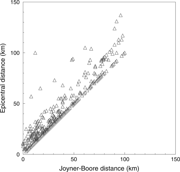
Correlations between R _epi and R _JB for the records used in the regression analyses.

Clearly, it is technically impossible for the difference between R _epi and R _JB to be greater than the rupture dimensions for a given earthquake. Figure 2 shows the differences between epicentral and Joyner-Boore distances, plotted against earthquake magnitude, together with the predicted estimates of total rupture length from the mechanism-independent relationship of Wells and Coppersmith (1994). The differences are generally within the 84^th percentile predictions of the rupture length at smaller magnitudes and below the median values for larger magnitudes; the latter feature is the result of the relatively low probability of an accelerograph station being located at the opposite end of a larger-magnitude earthquake with a unilateral fault rupture from the epicenter.

OPEN IN VIEWER

Figure 2.

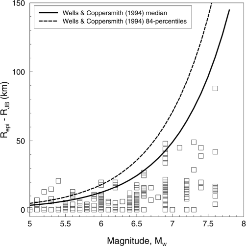
Differences between R _epi and R _JB values as a function of magnitude, compared with predicted fault rupture lengths from empirical relationship of Wells and Coppersmith (1994).

A troubling feature of the plot is the small number of data points for earthquakes with M_w < 5.5, for which the difference between the two distance metrics clearly exceeds the rupture length, suggesting an appreciable error in one (or both) of the distance estimations. The plot possibly makes the situation appear worse than is actually the case: The differences exceed the 84^th percentile estimates of the rupture length for only seven of 163 recordings in this magnitude bin. For the purposes of this study, these distances were not changed; the R _JB distances are equally likely to be in error as the R _epi values in this case.

The regression in Equation 1 using R _epi as the distance metric was performed in exactly the same way as in Akkar and Bommer (2010). We do not present the coefficients of the equations since the purpose of this exercise is only to illustrate the effects of using equations based on extended-source distance metrics with point-source event simulations. The previous plots show that the metadata needs improving before definitive R _epi -based models (and preferably R _hyp -based models) can be derived; that will be done within the context of producing the next generation of European ground-motion models that will take advantage of an expanded strong-motion database and improved metadata in terms of site characterization (e.g., Luzi et. al. 2010, Sandıkkaya et. al. 2010).

Figure 3 compares the standard deviations of the predictive model in terms of epicentral distance with those from the model of Akkar and Bommer (2010) based on the Joyner-Boore distance. The use of epicentral distance rather than Joyner-Boore distance results in marginally higher total sigma values at all response periods, which might be interpreted as a vindication for the tendency of most modern GMPEs to be based on extended-source distance metrics. The increase in sigma at short periods clearly comes from an increase in the within-event variability, which is consistent with the use of a distance metric that for larger magnitudes will often not be a good indicator of the separation of the point of observation and the source of seismic energy release.

OPEN IN VIEWER

Figure 3.

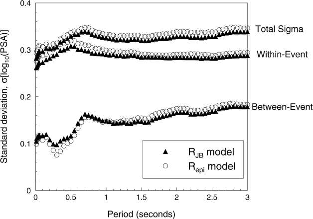
Standard deviations of log₁₀[PSA(T)] associated with Equation 1 using R _epi and R _JB as the distance metric, showing total sigma and the contributions from within-event and between-event variability.

Since the focus of this paper is the use of parallel pairs of GMPEs based on two different distance metrics, it is important that both equations are well adjusted and unbiased. Since the same functional form previously used and tested for our R _JB -based model was adopted for the R _epi -based model, it is worth examining the residuals of the new equation (Figure 4). The plots of the between-event and within-event residuals suggest that the R _epi model is unbiased. The relatively small numbers of data points at larger magnitudes and longer distances make it difficult to infer any dependence of the variability on these parameters. Moreover, since the R _JB equations of Akkar and Bommer (2010) included a constant (homoscedastic) sigma, for meaningful comparisons it is important to also have a similar sigma model for the R _epi equations.

OPEN IN VIEWER

Figure 4.

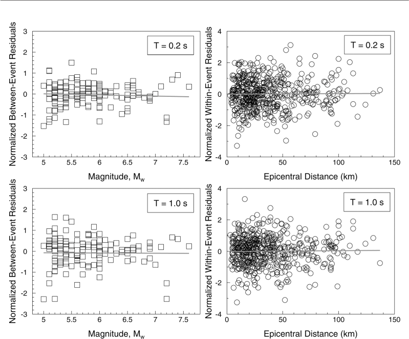
Normalized between-event residuals against magnitude (left) and within-event residuals against distance (right) for log₁₀[PSA(T)] for periods of 0.2 s (upper row) and 1.0 s (lower row) from the R _epi equations. The solid grey lines are the best straight line fit to the residuals.

Figure 5 shows the scaling factors implied by the two models for the influence of site classification (with respect to rock sites) and for the influence of style-of-faulting (with respect to strike-slip ruptures). The site effects coefficients are very similar for both models, whereas there are very large differences between the style-of-faulting factors for the two models, particularly for reverse ruptures. The lack of major differences in the implied site effect factors is to be expected since our equations do not include the influence of soil nonlinearity, hence soil amplification should not depend on distance. Moreover, the data for all three site classes are reasonably well represented by the corresponding records in magnitude-distance space. The larger differences observed in the right-hand panel may reflect the fact that the distribution of styles-of-faulting with magnitude is much less uniform. Most of the records from earthquakes of magnitudes greater than M_w 7 come from strike-slip events, with the exception of the three recordings from the reverse-faulting Tabas earthquake; the notable change in the scaling factors for reverse events is likely, in part, to be the result of the large R _epi -R _JB difference for the high-amplitude Tabas accelerogram. Faced with such large differences in the style-of-faulting coefficients, one could consider constraining the style-of-faulting factors from one model or the other (or using an average) so that these effects are common to both models. However, we consider it more appropriate to allow each model to be internally consistent.

OPEN IN VIEWER

Figure 5.

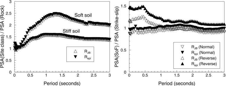
Scaling for stiff and soft soil sites with respect to rock from the two models (left), and scaling for normal- and reverse-faulting earthquakes from the two models (right).

Figure 6 compares predictions of median spectral ordinates from the two models, as a function of the indigenous distance metric of each equation, for three magnitudes representing the limits and central value of the range covered by the dataset. As would be expected, using the epicentral distance generally results in higher predicted accelerations for a given distance. This is because for the same data point the Joyner-Boore distance would be equal to or smaller than R _epi , thus reducing the ground-motion amplitudes predicted for a given distance. At M_w 5, the R _JB model actually predicts slightly higher accelerations (possibly an effect of the style-of-faulting scaling for strike-slip earthquakes compensating for the effects in Figure 5) but the differences between the predictions increase with increasing magnitude, with the R _epi model predicting much larger accelerations for moderate-to-large magnitudes. The differences decay with distance but persist even out to 100 km, especially for the larger earthquakes. The clear, and rather obvious, conclusion is the importance of using any GMPE with the correct distance definition.

OPEN IN VIEWER

Figure 6.

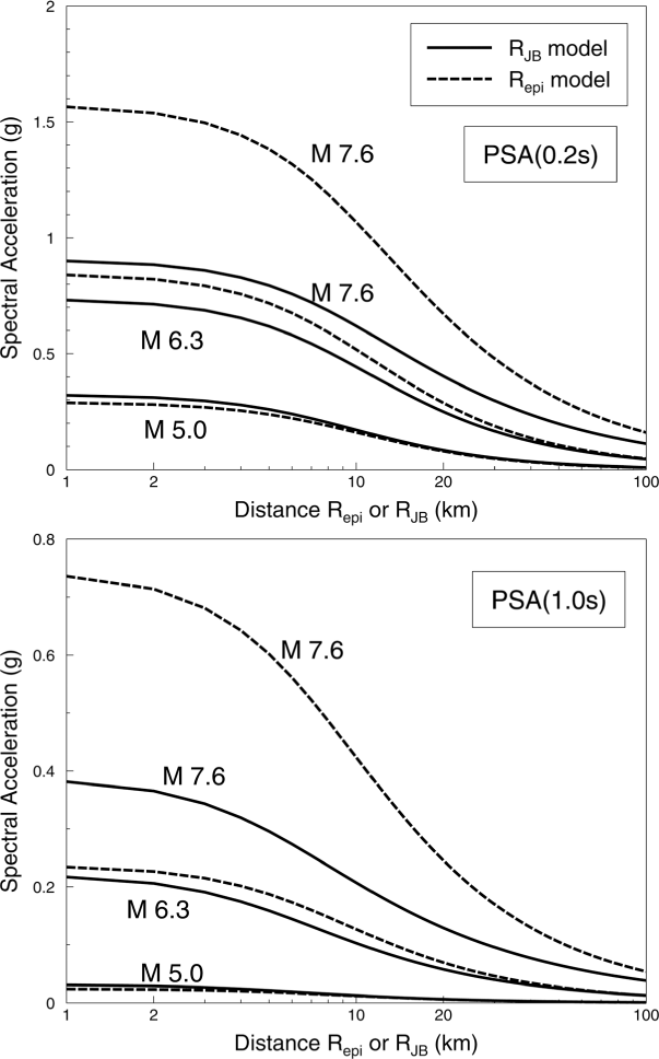
Predicted median spectral accelerations at 0.2 s (upper) and 1.0 s (lower) for strike-slip earthquakes of different magnitudes and rock sites at various distances, using each model with its own distance metric.

Before closing this section, there is a feature of Figure 6 that warrants discussion. One could argue that it is not physically reasonable that at the closest possible distance the R _epi model predicts ground-motion amplitudes that are so much greater than those obtained from the R _JB model. However, there is an internal consistency if one considers the amplitude of ground-motion intensity as a measure of the energy density of the shaking. For a large (say M_w 7.6) earthquake, the R _epi model predicts much a higher intensity of shaking (energy density) over areas defined by concentric annuli around the epicenter. For the same event, with a fault rupture length on the order of 100 km (Figure 2), the R _JB model predicts a lower intensity over much larger racetrack-shaped areas. The two models are therefore consistent in terms of the total predicted energy of the ground-motion field.

Implications for Hazard Calculations

The situation of interest here is performing PSHA with areal source zones of distributed seismicity (or smoothed seismicity models), in which earthquakes are modeled as epicenters, and GMPEs that employ a distance metric based on extended fault rupture sources such as R _JB and R _rup . One solution, as noted previously, is to simulate a number of virtual fault ruptures with lengths appropriate to the magnitude, and calculate the R _JB or R _rup values for the site, for each earthquake considered in the PSHA integrations. This is computationally demanding, not easily accessible to an analyst using software without such a capacity embedded, and the results obtained may be sensitive to choices such as fault orientations and the choice between unilateral and bilateral ruptures.

In the Introduction, it was noted that an alternative solution may be to use relationships between different distance metrics, such as those derived by EPRI (2004) and by Scherbaum et. al. (2004) using randomly located recording sites around hypothetical fault ruptures. Although conceptually elegant, there are many problems encountered in the practical application of these conversions, which are not limited to the large sigma penalty discussed previously. The key problem is as follows: Consider a single hypothetical earthquake event of magnitude M_w 6.3 simulated in the PSHA calculations as a point source (epicenter), for which the distance to the site (R _epi ) is 10 km. From Figure 6 it can be seen that the median value of PSA (0.2 s) from the R _epi model is 0.52 g; to obtain the correct value from the other equation, an R _JB value of about 7.5 km needs to be entered, which is consistent with the value obtained from the conversions presented in EPRI (2004). Now consider scenario events much closer to the site, and in the limiting case, directly below the site, for which R _epi takes a value of 0 km. If this value is entered into the R _JB equation, the spectral accelerations will be underestimated (Figure 6). However, in this case it is clearly not possible to obtain a smaller R _JB value that will yield the correct level of acceleration. Therefore, the use of empirical conversions such as those used by EPRI (2004) and Scherbaum et. al. (2004) simply breaks down for earthquake epicenters close to the site, which will nearly always need to be considered since the site will generally be situated within an areal seismic source zone. Since scenarios close to the site are likely to dominate the hazard in many cases (and particularly for low annual frequencies of exceedance), this is a very serious limitation.

The consequences of ignoring the inconsistency between the point-source scenarios and the extended-source distance metrics in most GMPEs can be illustrated by performing some simple PSHA calculations using both the Akkar and Bommer (2010) R _JB equations and the R _epi versions of the same equations derived for this study. The seismic hazard at a rock site located at the center of a circular area source with a radius of 100 km in terms of PSA (0.2 s) and PSA (1.0 s) is calculated using both equations, but in each case the R _epi distances calculated for the point-source scenarios are used as the distance in the equation without adjustment. For such an application, the R _epi equation is the “correct” model and the use of the R _JB model may be considered erroneous. Two different cases are considered: In both, the seismicity of the source is modeled by a truncated exponential recurrence relationship, with an activity rate of 0.1 and 5 and a b-value of 1 and 0.85, respectively, for the low- and high-seismicity scenarios; M _min was set at 5.0 for both cases but M _max values of 7.0 and 7.2 were employed for the two cases. The results are displayed in Figure 7, which shows hazard curves for these two spectral accelerations using the two GMPEs but entering unmodified epicentral distances as the distance in all cases.

OPEN IN VIEWER

Figure 7.

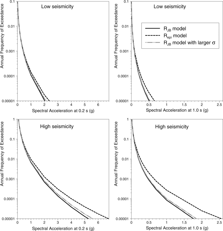
Seismic hazard curves for a rock site at the center of a circular seismic source with a radius of 100 km, considering only strike-slip earthquakes, for spectral accelerations at 0.2 s (left) and 1.0 s (right) obtained using the point-source and extended-source versions of the GMPEs; additionally, hazard curves obtained using the extended-source model but with the larger sigma values from the point-source model are shown as lighter dashed-dotted lines. The hazard curves are shown for two levels of seismic activity in the source, details of which are provided in the text.

The hazard curves in Figure 7 show that using GMPEs that employ R _JB (or R _rup ) for PSHA calculations with area sources as if the equations were based on distance metrics relative to point sources will lead to considerable underestimation of the seismic hazard. The same x-axis has been used for the low- and high-seismicity cases for each ground-motion parameter, which can make the underestimation in the former cases look relatively unimportant. However, following the procedure of Regulatory Guide 1.208 (NRC 2007) to obtain the ground-motion response spectra for the design of nuclear power plants, the hazard curve calculated for the low-seismicity region using the incorrect distance measure leads to a design value of PSA (0.2) of 1.08 g as opposed to the correct value of 1.25 g, an underestimation of 13%. For the 1-second response ordinate, the underestimation of the correct design acceleration is 23%.

Some of the divergence between the pairs of hazard curves from the R _epi -based and R _JB -based equations in the frames of Figure 7 is clearly due to the slightly larger standard deviation of the R _epi -based equations, but the major contributor is the difference in the median predictions. The degree of underestimation by the R _JB -based model will depend on the degree of activity in the source and the maximum magnitude, since the difference between point-source and extended-source distance metrics grows with increasing earthquake magnitude. The sensitivity to magnitude makes the difference more pronounced for longer-period spectral ordinates and it increases with reducing annual frequency of exceedance. Therefore, it is possible that for low seismicity regions and the return periods commonly used as the basis for defining earthquake actions in building codes (500–2,500 years), the errors in the hazard estimates may be considered negligible, especially if the focus is on short-period parameters such as peak ground acceleration (PGA). At the return periods relevant to the seismic design of safety-critical facilities, this error cannot be ignored and remedial measures are required to avoid the underestimation that results from inappropriate combinations of earthquake source models and source-to-site measures in GMPEs.

Conclusions

The state-of-the-art in ground-motion prediction models generally involves the use of an extended-source distance metric. Such measures improve the modeling of seismic radiation from future fault ruptures that may have lengths of several tens of kilometers. However, nearly all seismic hazard analyses involve representations of future earthquakes as point sources, either through integration over areal source zones or smoothed seismicity. Point-source (epicenter) simulations can be enhanced to include simulations of virtual extended ruptures for consistency with distance metrics such as R _JB , R _rup , and R _seis used in many GMPEs. Such adaptations are computationally demanding and not easily implemented. In current practice, using widely available PSHA codes, it is not at all uncommon for GMPEs based on extended-source measures to be combined with earthquake simulations as epicenters with no adjustments, which tends to produce significantly underestimated hazard.

We propose that the simplest and most consistent solution to this problem is for all GMPEs to be derived and presented in pairs of models, one using the analysts’ preferred extended source metric—or even combination of metrics, as in some recent models (e.g., Abrahamson and Silva 2008)—and another using a point-source metric, for which our preference would be hypocentral distance, R _hyp . We recommend that this be added to the list of desirable features of GMPEs presented in Figure 5 of Bommer et. al. (2010).

In addition to the advantages such consistent pairs of ground-motion models would offer to PSHA, they could also be useful for ShakeMap applications (e.g., Wald et. al. 1999). Immediately following an earthquake, when only the epicentral location has been determined, the ground-motion field could be estimated using the GMPE based on R _epi or R _hyp ; once information becomes available regarding the location and size of the fault rupture, the shaking distribution could be updated using the GMPE based on an extended-source measure of distance.